1. Introduction
Ferromagnetic materials are extensively employed in petroleum pipelines, bridges, and railway tracks because of their outstanding mechanical properties. It is inevitable that cracks, holes, dislocations, and other defects will appear in ferromagnetic components during manufacturing or service, which will seriously affect their performance and even lead to safety accidents. Quantitative nondestructive testing and evaluation of defects are crucial for ensuring equipment safety. Timely detection of defects and maintenance or replacement can effectively prevent safety accidents and economic losses. Metal magnetic memory detection technology has drawn considerable interest from researchers since it was proposed. It is a passive nondestructive testing method without an additional excitation magnetic field, it is easy to operate, and it has unique advantages in stress and defect detection in early stages. A series of theoretical and experimental studies have been carried out to investigate this method in recent years [
1,
2].
In terms of theoretical research, Jiles [
3] developed a theoretical model of magnetomechanical effect, which has been widely used to interpret experimental phenomena of the magnetic memory method. Li [
4,
5,
6,
7] extended the Jiles model by incorporating the Rayleigh law, thereby providing a more accurate description of the influence of stress on magnetization. Wang [
8] established a magnetic–elastic–plastic magnetization model by considering the influence of elastic–plastic deformation and analyzed how stress affects magnetization at different deformation stages. Shi [
9] proposed a general nonlinear magnetomechanical model for ferromagnetic materials under a constant weak magnetic field and compared it with the classic Jiles model; their model could more accurately predict the magnetization changes under the action of applied compressive stress.
In terms of experimental research, Bao [
10] studied the normal and tangential components of the MMS on the surfaces of smooth specimens made of different ferromagnetic materials (e.g., Q235, Q345, and 1045 steels) under elastic and plastic deformations. The research revealed that the residual magnetic signal behaviors of various types of steel at different deformation stages were significantly different. Yao [
11] studied changes in the normal component of the surface magnetic memory signal of Q235 steel specimens with a circular hole defect under different stages of tensile and compressive stress, finding that the gradient of the normal component of the magnetic memory signal was more sensitive to stress compared to its peak value. Bao [
12] studied variations in the normal and tangential components of residual magnetic signals of U75V steel specimens containing circular holes and U-shaped defects. This findings revealed that the tangential component B
x of the surface magnetic field exhibits greater sensitivity to local stress concentration compared to the normal component B
z, and the defect-induced MMS can correctly identify stress concentration but is not sensitive enough to the geometric shape of the defect. Roskosz [
13] studied the correlation between MMS and stress distribution of ferromagnetic materials under a tensile load, and they proposed a method for evaluating residual stress using an MMS gradient. Research conducted by Liu [
14] on pipeline weld characteristics demonstrated that the peak–valley amplitudes of normal and tangential magnetic memory signals exhibit a positive correlation with metal phase transformation and residual stress magnitude, but they show an inverse relationship with probe lift-off distance. Dimove [
15] used a magnetic memory detection method to detect early stress concentration areas in nuclear power pipelines. Shi [
16] and Bao [
17] provided a detailed overview of metal magnetic memory detection technology from the perspectives of magnetomechanical effect, influencing factors of the MMS, damage evaluation criteria, and future development directions. Su [
18] summarized research progress in magnetic memory detection technology in the field of civil engineering in recent decades, discussing the current problems and proposed future challenges.
These studies have promoted the development of magnetic memory detection technology, but shortcomings persist. These limitations include the following: the theoretical research on magnetic memory detection technology is not systematic enough; most existing models analyze MMS from the perspective of magnetomechanical coupling or magnetic charge theory, and there have been few models that comprehensively consider the relationships between stress, magnetization, defects, and magnetic field strength. Additionally, most experimental studies analyzed the normal and tangential components of MMS, ignoring the third directional component and not fully utilizing all of the information of the magnetic memory detection signals, which can easily lead to missed detection or misjudgement in practical applications. Furthermore, most experiments only provide the distribution of MMS on a fixed measurement line, without providing the 2D or 3D distribution of MMS.
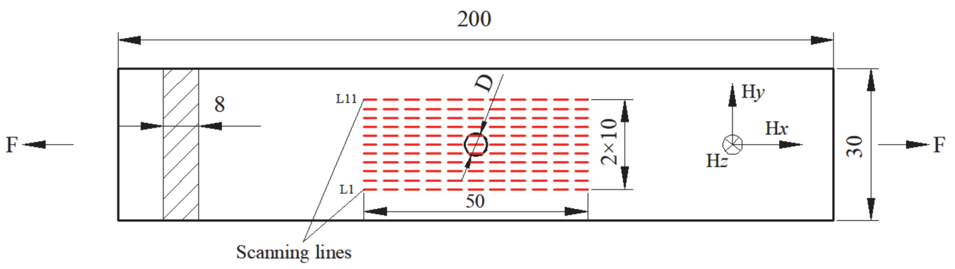
In this research, the 3D MMS on the surface of specimens without and with a circular hole defect were systematically investigated using tensile tests. Three-dimensional MMS characteristic parameters were extracted, and the relationship between magnetic parameters, applied load, and defect size was quantitatively analyzed. In addition, an evaluation method for defect size and applied load was introduced via a Lissajous graph and nonlinear fitting equation. Finally, the key findings of this study were discussed.
3. Results and Discussion
3.1. Experimental Reproducibility and Reliability
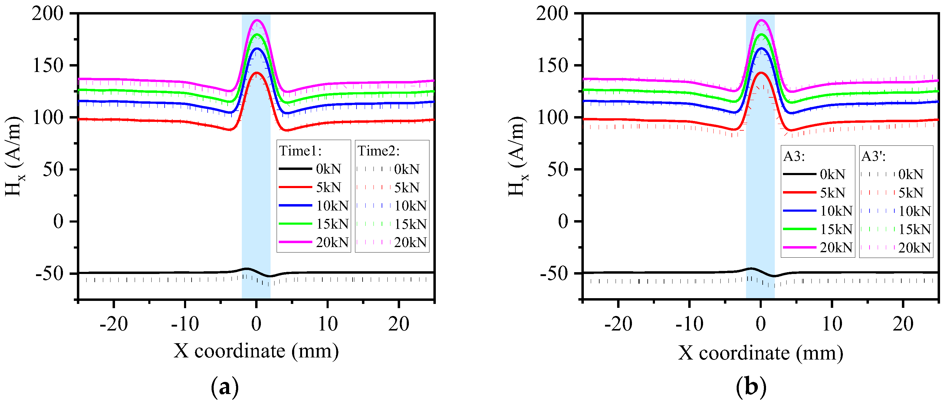
To evaluate the stability of the experimental setup and methodology, reproducibility tests were performed on specimen A3 under identical conditions. The initial measurement (Time1) and a repeated measurement (Time2) were compared. As shown in
Figure 3a, the H
x variations along scanning line 6 exhibit strong agreement across different loading conditions, confirming the high reproducibility of this testing approach. In addition, under the same experimental conditions, a reliability experiment was conducted using A3’ for measurement, and the experimental results were compared with the measurement results of A3.
Figure 3b shows the variations in H
x along scanning line 6. One can observe that the measurement results demonstrate good consistency between specimens A3’ and A3, indicating that the experimental setup and scheme have high reliability.
3.2. Experimental Results of the Specimen Without Defects
3.2.1. 3D MMS Morphology Graph
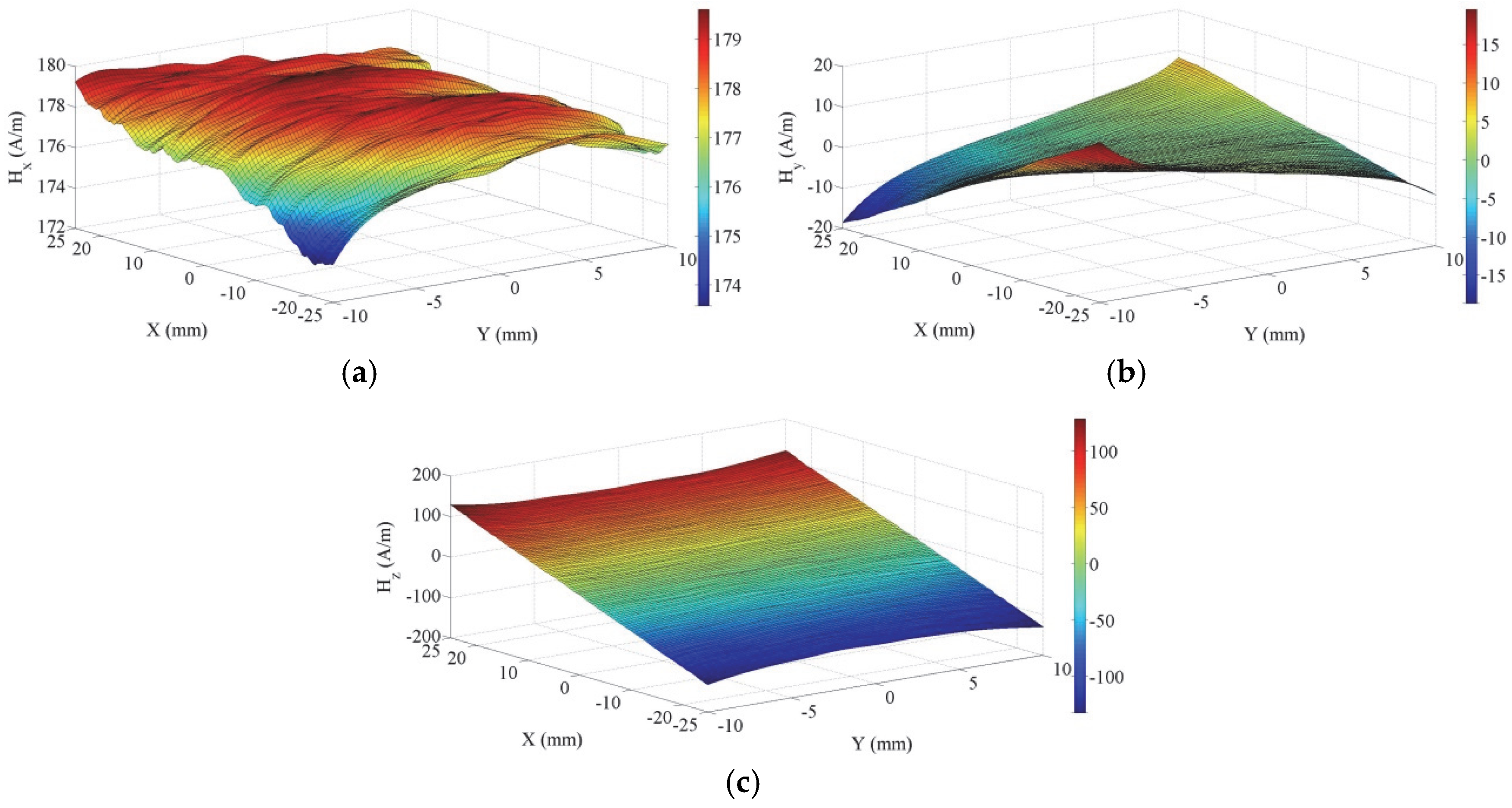
Figure 4 shows the 3D MMS morphology of A0 without defects under a tensile load of 20 kN in the measuring area. From the figure, one may observe that H
x remains relatively constant along the X-axis and Y-axis, with values ranging from 174 A/m to 179 A/m. H
y is approximately the zero plane. H
z exhibits an oblique straight line along the X-axis, with values ranging from −110 A/m to 110 A/m, whereas it keeps a constant value along the Y-axis direction.
3.2.2. 3D MMS Along the Scanning Line
Figure 5 shows the variations in the 3D MMS of A0 along scanning line 6 under different tensile loads. It can be seen that the H
x curves, parallel to each other, have almost zero slope. Meanwhile, the curves show a movement towards the positive direction of the vertical axis. The magnetic field strength increases from 137 A/m to 177 A/m with load increases from 5 kN to 20 kN. The H
y curves show approximately horizontal lines. The H
z curves vary almost linearly. At 0 kN, the H
z curve is approximately a horizontal line. The slope of the H
z curves gradually increases with increasing load. Moreover, all curves intersect at the point (0,0) and rotate clockwise with an increase in the applied load.
3.3. Experimental Results of the Specimen with a Circular Hole Defect
3.3.1. 3D MMS Morphology Graph
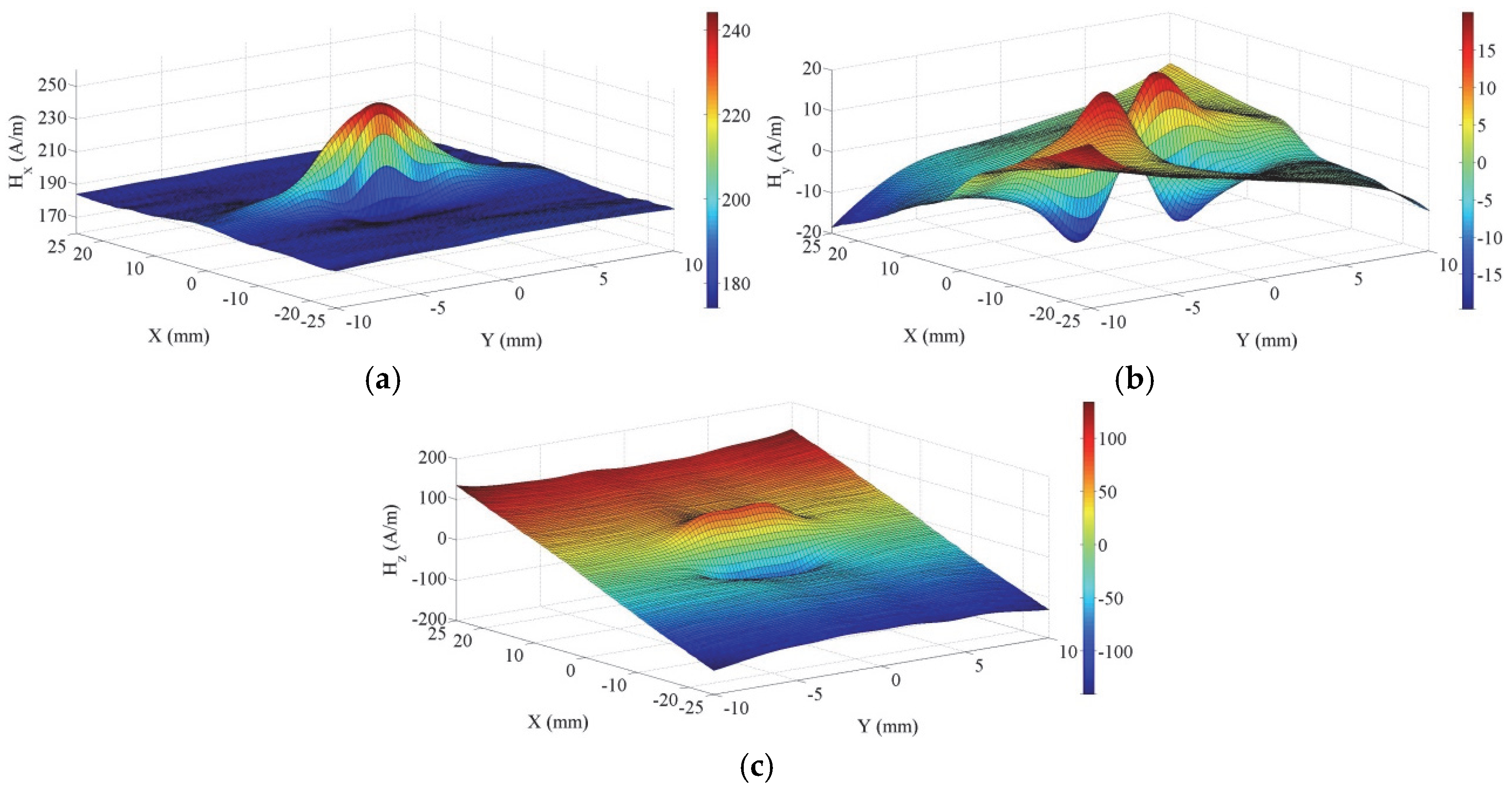
Figure 6 shows the 3D MMS morphology of A3 with a circular hole defect under a tensile load of 20 kN in the measuring area. One may observe that H
x exhibits an abnormal magnetic change around the circular hole defect area and a peak shape form in the middle of the graph, where the peak value is 240 A/m. H
x is approximately a plane on both sides of the defect, with a value of 180 A/m. H
y exhibits four peaks and valleys in the defect area, with symmetry when rotated 180° around the defect center. The two positive peak values are 20 A/m, and the two negative valley values are -20 A/m. As it moves away from the defect area, its value fluctuates around 0 A/m. At X = 0 or Y = 0, its value is similar to 0 A/m, with no nonlinear variation. H
z shows a peak–valley trend along the X-axis, ranging from −120 A/m to 120 A/m. The closer it is to Y = 0, the larger the peak–valley value is; the farther it is from Y = 0, the smaller the peak–valley value is. The center of the peak–valley variation corresponds to the center of the hole defect.
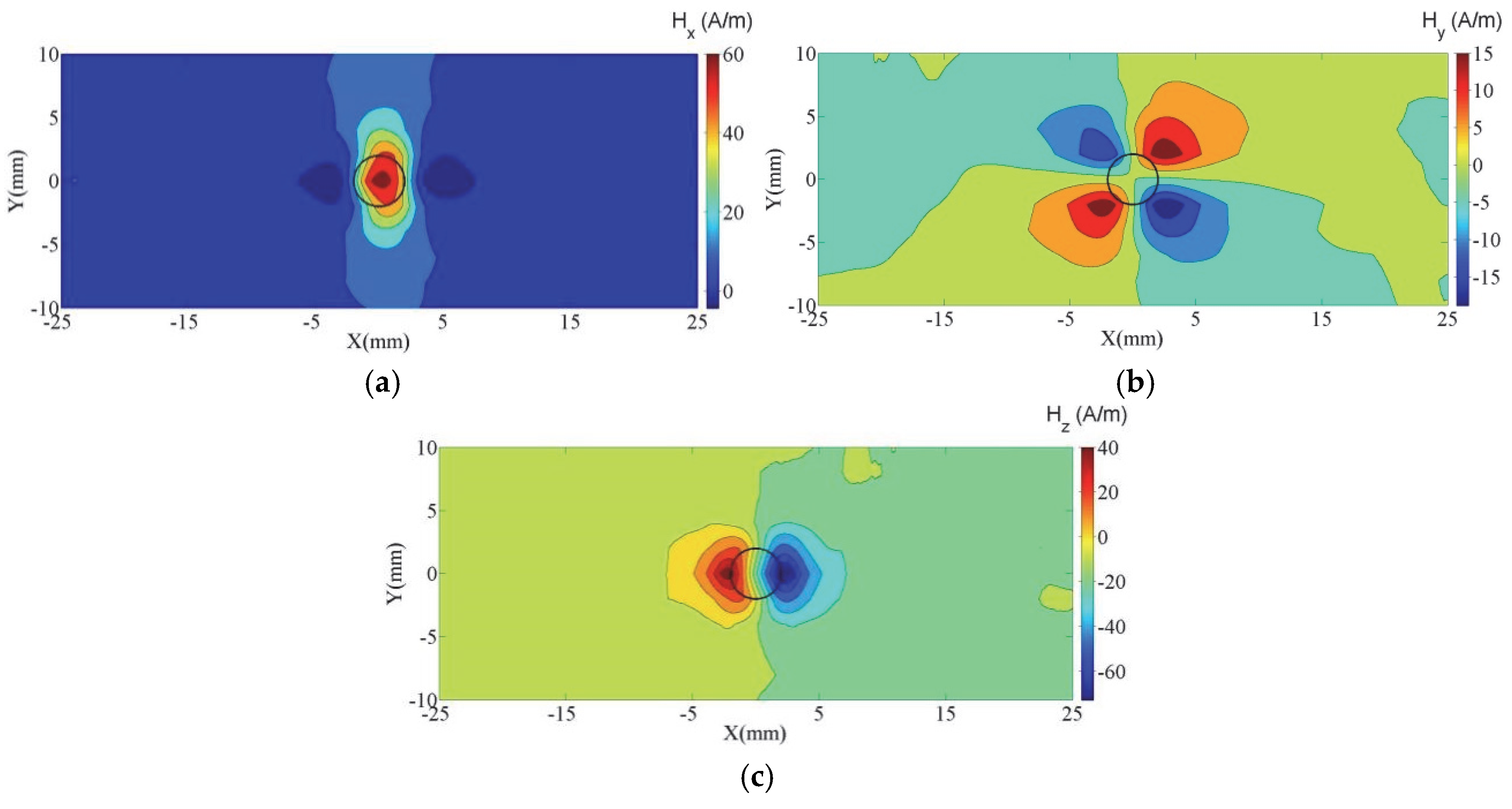
Figure 7 shows the 2D contour map of the 3D MMS of A3 under a tensile load of 20 kN in the measuring area. All signal values are subtracted from the 3D MMS values of A0 under a load of 20 kN. It can be seen that under this tensile load, H
x exhibits peaks in the defect area of the circular hole, with a peak value of 60 A/m. The peak value corresponds to the center position of the defect, and the profile of the peak region is close to the outline of the circular hole defect. Additionally, H
x has extreme regions in the form of grooves on both sides of the peak value. H
y exhibits positive and negative peak–valley regions at the four corner positions of the circular hole defect. The positive peak values in the 1st and 3rd quadrants are 15 A/m, whereas the negative valley values in the 2nd and 4th quadrants are −15 A/m. The H
z exhibits positive and negative peak–valley changes at the left and right edges of the circular hole defect and crosses the zero point at the center of the circular hole defect. The positive valley value is 40 A/m, and the negative valley value is −60 A/m.
3.3.2. 3D MMS Along the Scanning Line
Effects of Load
Figure 8 shows the 3D MMS of A3 along scan line 6 under tensile loads from 0 kN to 20 kN. It can be seen that as the H
x curves move upwards, abnormal magnetic changes occur in defect areas, and a peak is located in the defect center. The peak value increases from 193 A/m to 243 A/m when the tensile load increases from 5 kN to 20 kN, and the reference magnetic value away from the defect area increases from 148 A/m to 187 A/m. The H
y curves display approximately horizontal lines, which is the main reason why this component signal is often ignored. The H
z curves exhibit peak–valley variations near the center of the defect, with the center of the peak–valley variation corresponding to the center of the circular hole defect. The peak–valley value increases with increasing load, while the peak–valley spacing keeps a constant value. The curves rotate clockwise along the center point of the specimen with increasing loads, and the slope of the curves in the middle of the specimen are significantly greater than that in other areas, with a slope value of −37.22 A/mm. Similar phenomena can be observed from specimens with different defect sizes.
At present, theoretical and experimental research on magnetic memory detection technology mostly focuses on the H
x and the H
z of MMS. There are few studies on H
y, and it is often overlooked because the H
y value on the scanning line passing through the defect center is 0 A/m. The nonlinear changes in H
x and the H
z are used to clearly determine the presence of defects, as well as the X-directional position and size of defects. However, using only H
x and H
z could not reflect the Y-directional position of defects, as H
y contains the Y-directional position information of defects. For this purpose, we have provided the MMS variations in the H
y along scanning lines 5 and 7 on both sides of the defect center of A3, as shown in
Figure 9. The H
y curves are not symmetrical along the center of scanning line 6, and they exhibit magnetic anomalies on both sides of the scanning line 6, showing peak–valley changes. The peak–valley values increase with increasing load, but the peak–valley spacing keeps a constant value. When the scanning line is located on the negative half of the Y-axis (scanning line 5), the H
y curves initially reach their maximum value and then their minimum value. In contrast, when the scanning line is located on the positive half of the Y-axis (scanning line 7), the H
y curves initially reach a minimum value and then a maximum value. This result indicates that using H
y could determine the position of defects in the Y direction. The combined use of three components of MMS is beneficial for achieving an accurate evaluation of defect location and size parameters.
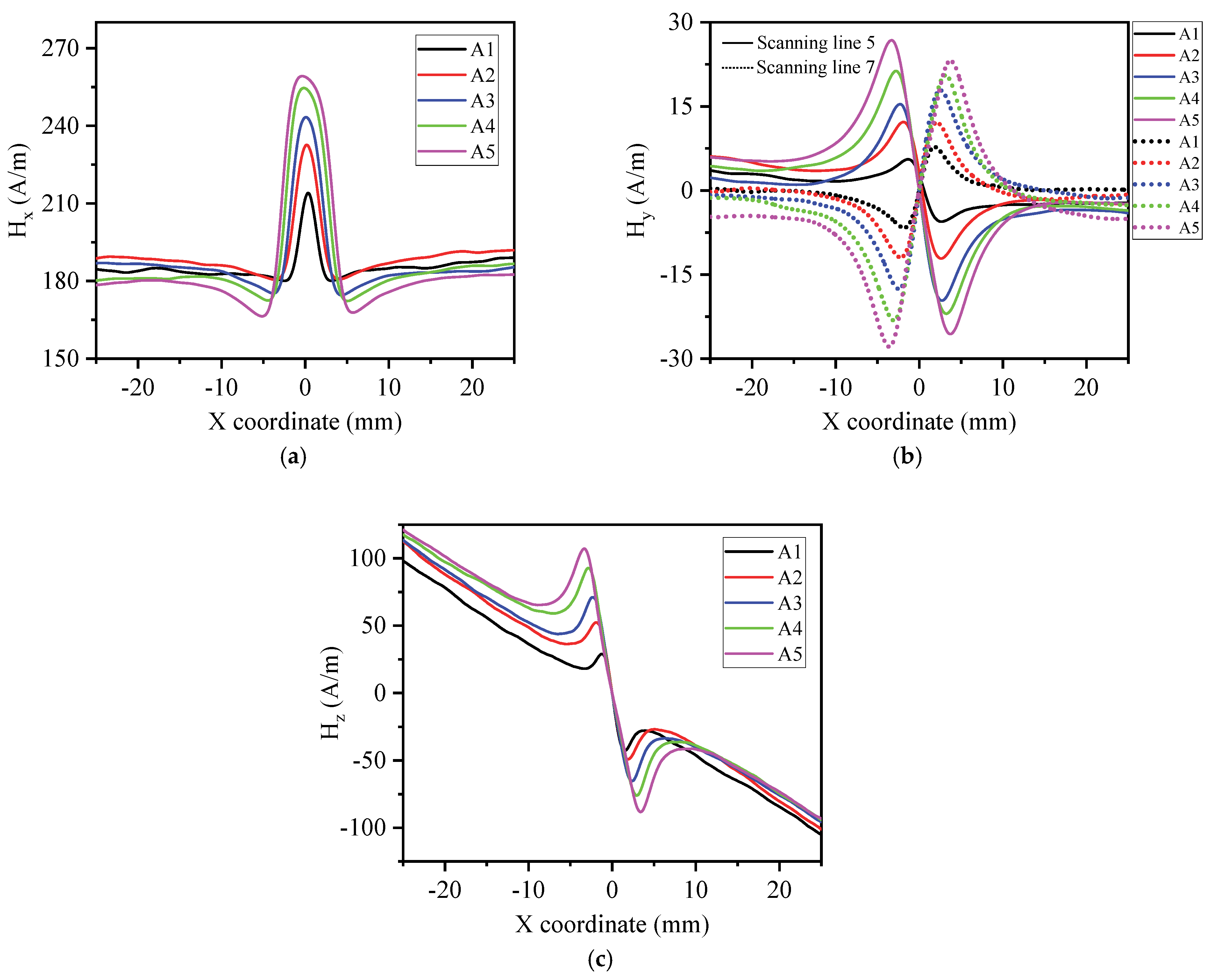
3.3.2.2 Effects of Defect Size
Figure 10 displays the effects of different circular hole defect sizes on the 3D MMS under a load of 20 kN. H
x and H
z are the measurements of scanning line 6, and H
y reflects the measurements of scanning lines 5 and 7. One can see that the peak–valley value and peak–valley spacing of the H
x, H
y, and H
z curves increase with increasing defect size. The slope of H
z in the defect region keeps a constant value of approximately −37.22 A/m/mm.
3.4. Theoretical Interpretation of Experimental Results
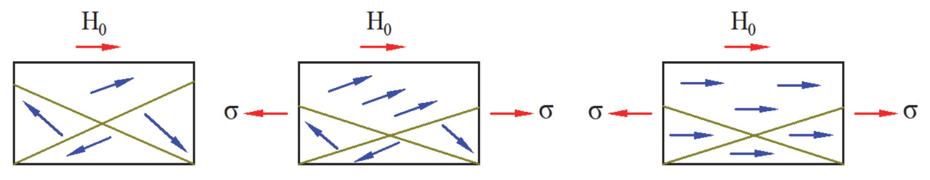
In the above analysis of the experimental results of the specimen without and with a circular hole defect, one can see that the specimens are magnetized under a tensile load, and the surface MMSs exhibit different characteristics. Below is a micro-structure analysis of the magnetomechanical coupling mechanism of ferromagnetic materials under a tensile load. As is well known, ferromagnetic materials are composed of multiple magnetic domains, each with a volume of 10–8 to 10–11 m
3, containing approximately 1012 to 1015 atoms. Due to thermodynamic motion, domain moments are randomly distributed in the initial state and do not exhibit magnetism externally. When the specimen is in a geomagnetic field environment, lattice symmetry is broken inside the material, causing reversible displacement of domain walls and forming an initial magnetization state, as shown in
Figure 11. When a tensile load is applied simultaneously, based on the theory of piezoelectric effect [
20], a non-uniform stress field is generated inside the material, and its stress energy density can be expressed as follows:
where
λs is the magnetostriction coefficient,
σ is the stress tensor, and
θ is the angle between the stress direction and the magnetization direction. To achieve minimization of the total free energy (including exchange energy, magnetic crystal anisotropy, demagnetization energy, and magnetoelastic energy) in ferromagnetic components, the magnetic domains in the material will undergo reorientation by increasing the magnetoelastic energy to counteract the increase in stress energy. During this process, the volume of magnetic domains with smaller angles to the direction of tensile load grows, and the magnetization strength along the load direction significantly increases. When the load exceeds the critical value, the magnetic domain rotates and eventually becomes parallel to the direction of the load. Even when the load is removed, the irreversible orientation of magnetic domains due to changes in the microstructure of the stress concentration zone still maintains the magnetization state.
In addition, under the co-action of the tensile load and the geomagnetic field, the 3D MMS exhibit pronounced magnetic anomalies at the site of hole defects in the specimen. The physical mechanism can be attributed to the discontinuity of the material’s geometric structure caused by defects, which directly leads to a sharp change in local magnetic permeability. According to the boundary conditions of Maxwell’s equations:
At the interface, the tangential component of the magnetic field strength H is continuous, while the normal component of the magnetic induction strength B is continuous. Geometric discontinuity causes the continuity of the tangential component of the magnetic field to be disrupted, forming a magnetic flux density discontinuity zone.
The generation of 3D MMS can be explained by the following theory. Circular hole defects disrupt the continuity of the material, resulting in a 3D asymmetric distribution of the local stress field. According to magnetoelastic theory, 3D stress promotes the movement of domain walls and the rotation of magnetic moments, causing stress magnetization in the specimen and satisfying the extended Jiles [
3] magnetomechanical coupling equation, which can be expressed as follows:
where
i represents the three directions of x, y and z. In addition, volume magnetic charges and surface magnetic charges were generated at the defect. According to the magnetic charge theory [
21], the accumulation of magnetic charges caused a 3D leakage magnetic field, H
x, H
y, and H
z on the surface of the specimen. Additionally, the magnetic charge density increases nonlinearly with increasing tensile load, causing greater distortion of the magnetic field in the defect region. Moreover, the larger the defect volume is, the greater the magnetic field intensity will be. The symmetry observed in the H
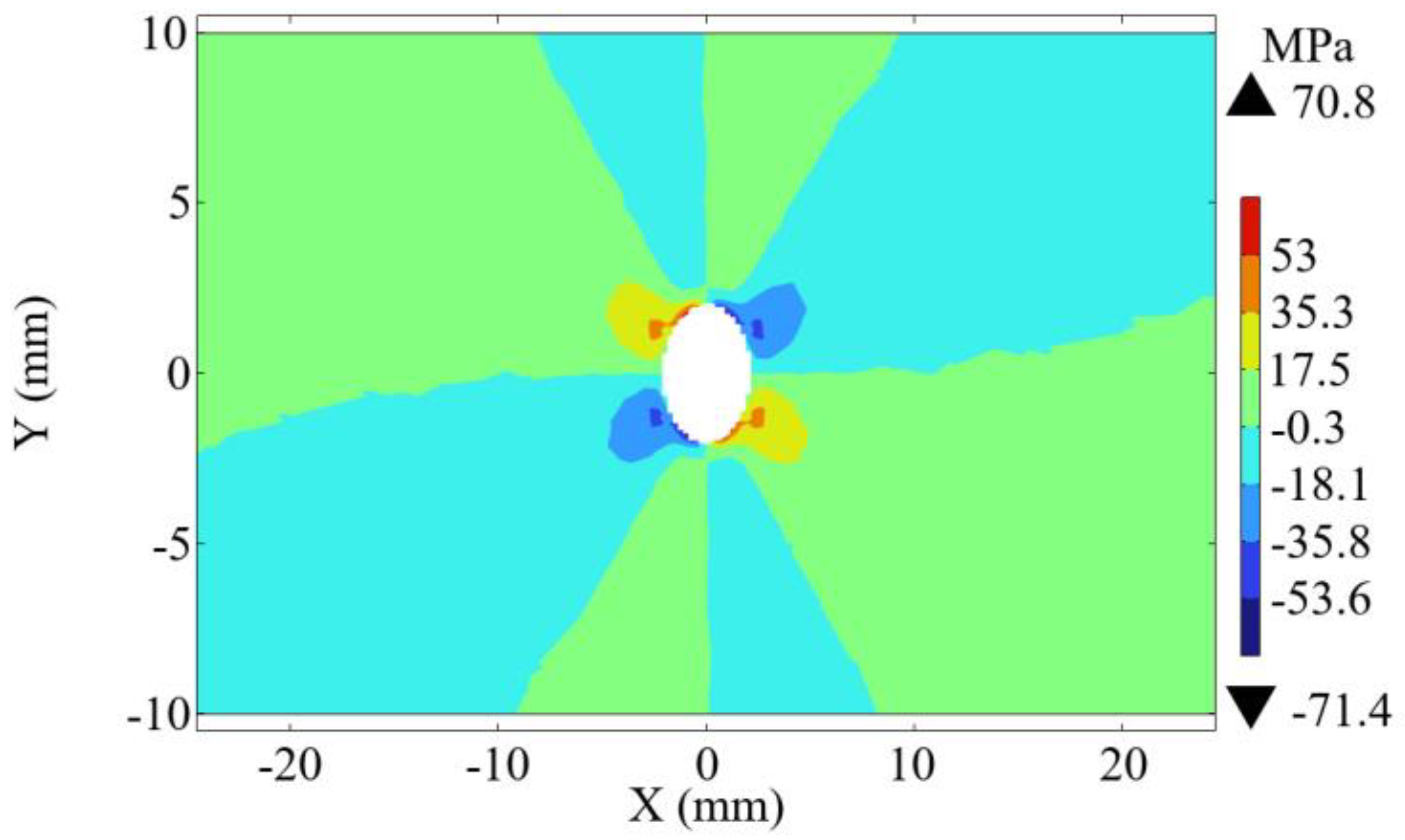
y component of MMS arises from the shear stress distribution within the specimen. Finite element method (FEM) analysis of the surface stress field in specimen A3 under 20 kN is shown in
Figure 12. One can see a distinct quadrant-based pattern: compressive stress dominates in the 1st and 3rd quadrants, while tensile stress prevails in the 2nd and 4th quadrants. This symmetric stress distribution drives the accumulation of positive magnetic charges in compression-dominated regions and negative charges in tensile zones, thereby inducing the characteristic quadrant symmetry of the H
y signal.
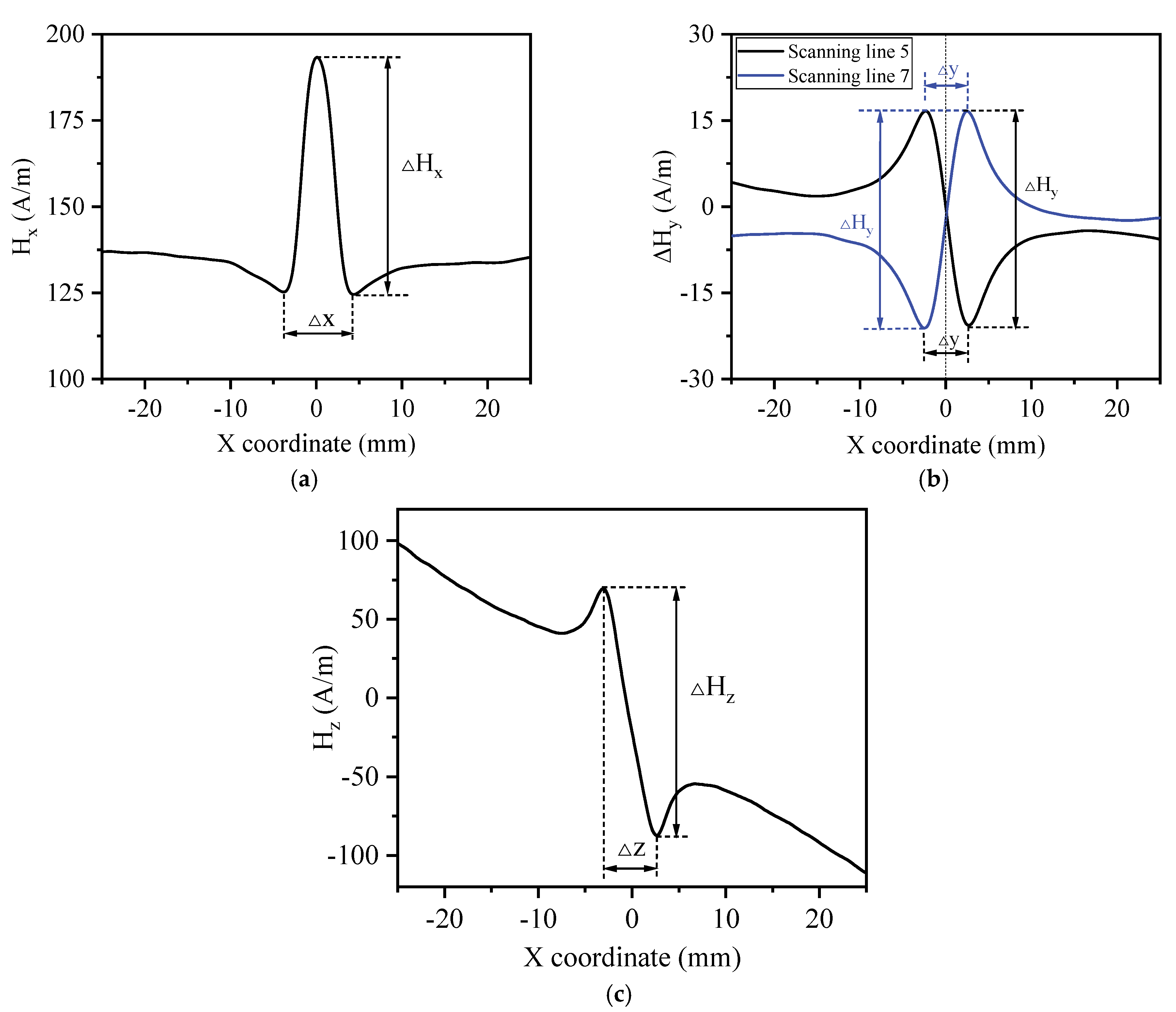
3.5. Definition of 3D MMS Characteristic Parameters
For a quantitative investigation of how applied load, circular hole defect size, and other factors influence 3D MMS, the following characteristic parameters of MMS are defined, as shown in
Figure 13, which are the peak–valley difference ΔH
x and peak–valley spacing Δx of H
x, peak–valley difference ΔH
y and peak–valley spacing Δy of H
y, and peak–valley difference ΔH
z and peak–valley spacing Δz of H
z. The main reason for using these features is that we noticed significant changes in these features with respect to the various loads, defect locations, and sizes in previous MMS analysis. Peak–valley spacing characterizes the distortion interval of MMS, whereas peak–valley difference characterizes the distortion intensity of MMS.
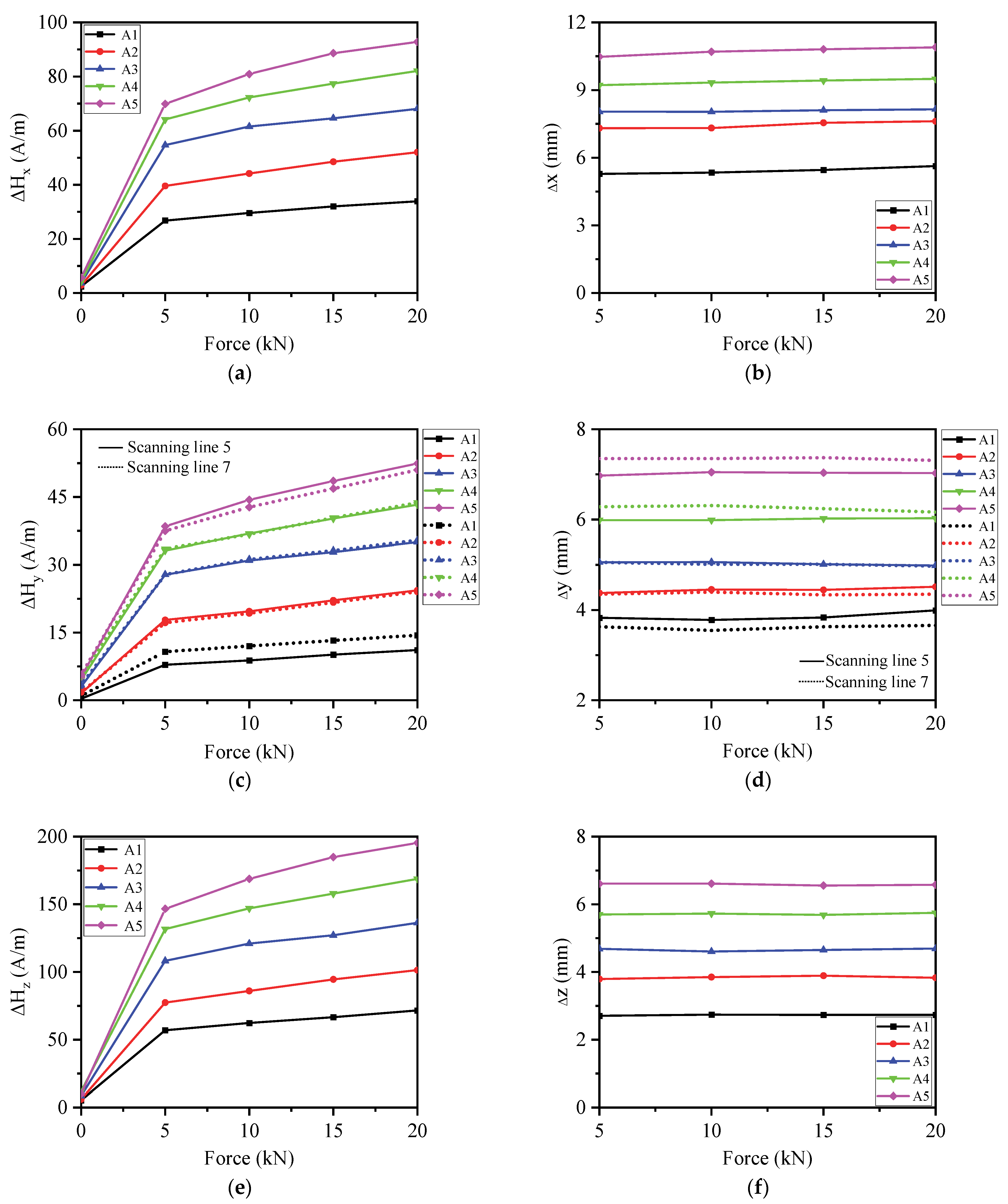
3.5.1. Effects of Load on 3D MMS Characteristic Parameters
Figure 14 further analyzes the effects of load on 3D MMS characteristic parameters. The results show that the magnetic parameters ΔH
x, ΔH
y, and ΔH
z increase with the increase in load, but their corresponding peak–valley spacings, Δx, Δy, and Δz keep a constant value with the increase in load. The peak–valley difference can be used to characterize the load level.
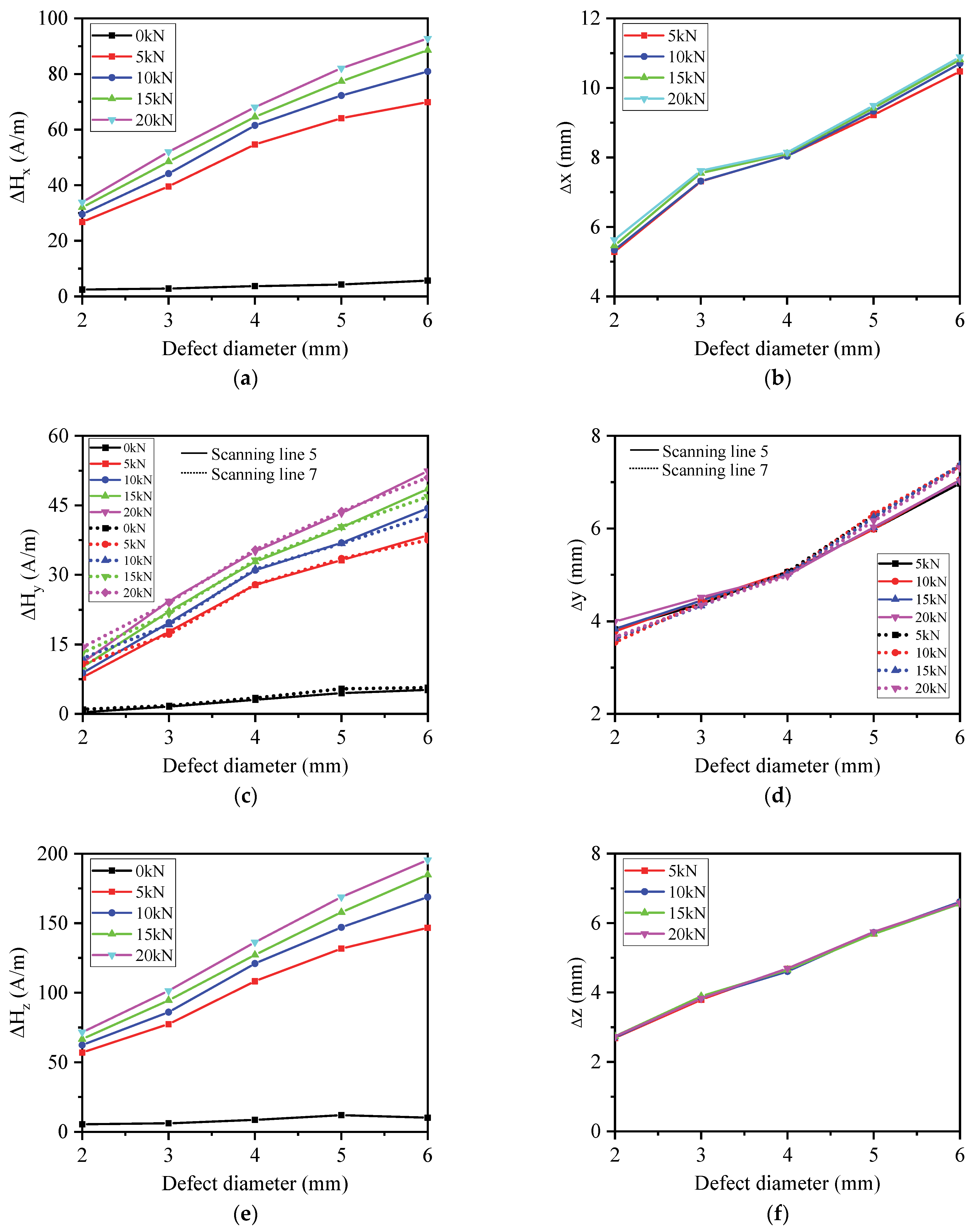
3.5.2. Effects of Defect Size on 3D MMS Characteristic Parameters
Figure 15 displays the effects of defect size on 3D MMS characteristic parameters. The results indicate that both the magnetic parameters ΔH
x, ΔH
y, ΔH
z and their corresponding peak–valley spacing Δx, Δy, and Δz increase with increasing defect size. The defect size can be characterized by these parameters.
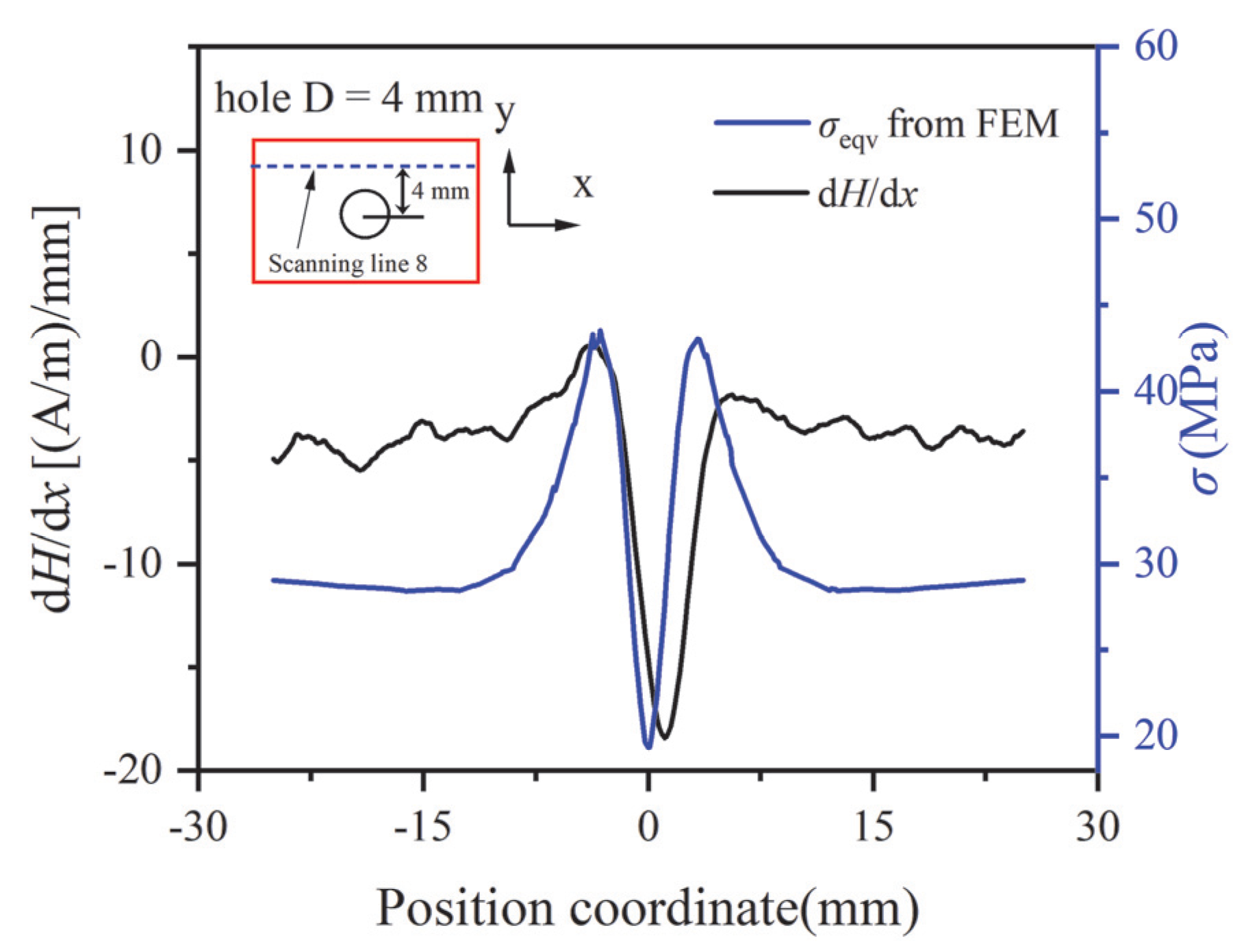
3.6. Relationship Between Stress Distribution and 3D MMS Characteristic Parameters
Subsequently, we analyzed the relationship between MMS and stress distribution. In reference [
22], Sablik established the equivalent stress expression for biaxial stress as follows:
Research has found that a MMS gradient can better characterize stress distribution than MMS. References [
13,
19,
23] define the sum of the 3D MMS gradient along the X-direction, expressed as follows:
Figure 16 shows the 3D MMS gradient along the X-direction and the equivalent stress of A3 along scanning line 8 obtained through FEM simulation. Good correspondence was observed between the gradient and the equivalent stress. Therefore, d
H/d
x can serve as a judgement of stress distribution along the X-direction.
3.7. Application of Lissajous Graph in Defect Size Evaluation and Stress Analysis
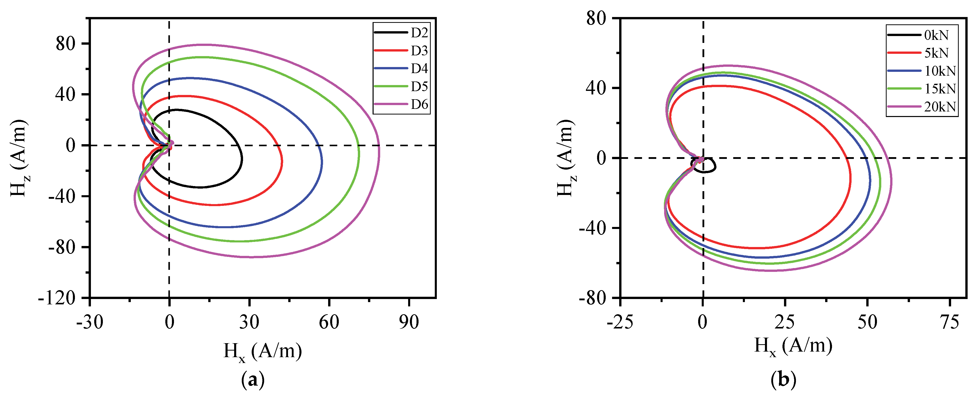
The shape formed by a particle undergoing harmonic motion in the X and Y axes is the Lissajous figure. Upon observing the curves of Hx and Hz of the MMS, one can see a sudden peak in the Hx curve, whereas the Hz curve showed a sudden peak with opposite signs before and after the zero crossing point. Moreover, the MMS changed smoothly when the location was far away from the defect, exhibiting the characteristics of particle changes mentioned above. Therefore, by combining the curves of Hx and Hz, a stable closed area pattern similar to the Lissajous figure was obtained. This not only reflects the characteristic states of both components of the MMS but also avoids a loss of information with defect features in stress concentration zones.
Figure 17 shows the effects of defect size and load on the 2D detection curves generated from H
x as the horizontal axis and H
z as the vertical axis. It can be seen that the area of the stable closed Lissajous graph increases with increasing defect size and applied load. Consequently, the defect size and the degree of stress concentration can be evaluated based on the Lissajous figure.
3.8. Defect Size Evaluation
Defects can seriously affect the performance of ferromagnetic components. Accurate evaluation of defects can help monitor the health of components, maintain or replace them in a timely manner, and avoid safety accidents. Next, we will use a nonlinear fitting method to quantitatively evaluate the defect size. Through the above analysis, it can be concluded that the characteristic parameters of MMS are strongly associated with both the applied load and defect size. Therefore, we can express the magnetic characteristic parameters as a function of the applied loading and defect size:
where Δ
H is the mean value of the peak–valley difference of the three directional components of the MMS, f(
F) represents a function related to the load, and f(
D) represents a function related to the defect size.
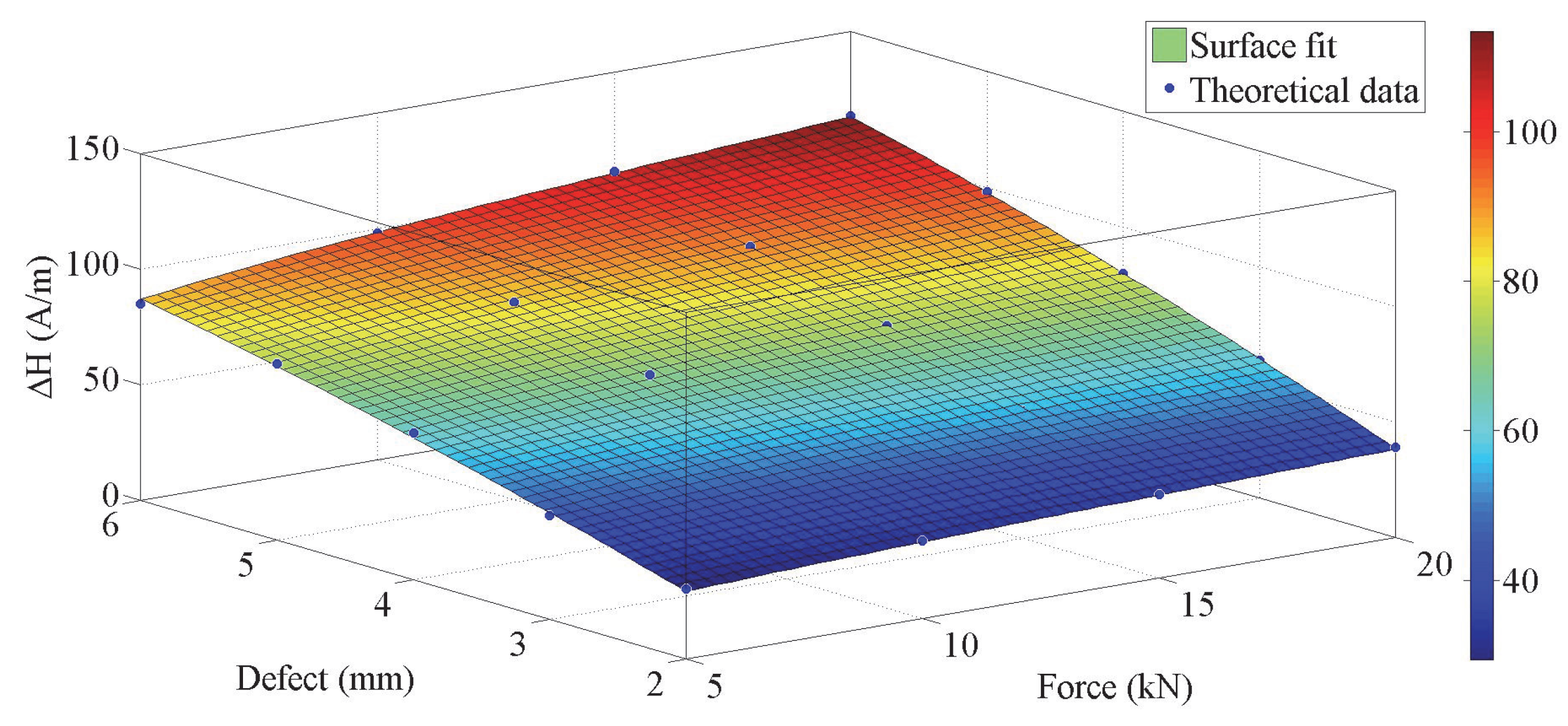
According to the experimental measurement data,
Figure 18 shows the nonlinear fitting surface between the loading, defect size, and 3D MMS characteristic parameter Δ
H. Through nonlinear fitting, the nonlinear functional relationship among them can be described as follows:
The equation coefficients are as follows: b1 =5.348 × 10⁻², b2 = − 2.727 × 10⁻³, b3 = 5.674 × 10⁻⁵, c0 = 1.39, c1 = 19.24, c2 = −0.7757, where F is the value of applied loading, and D is the value of defect size.
Based on this relationship, the defect size can be evaluated when the applied load
F and 3D MMS characteristic parameter Δ
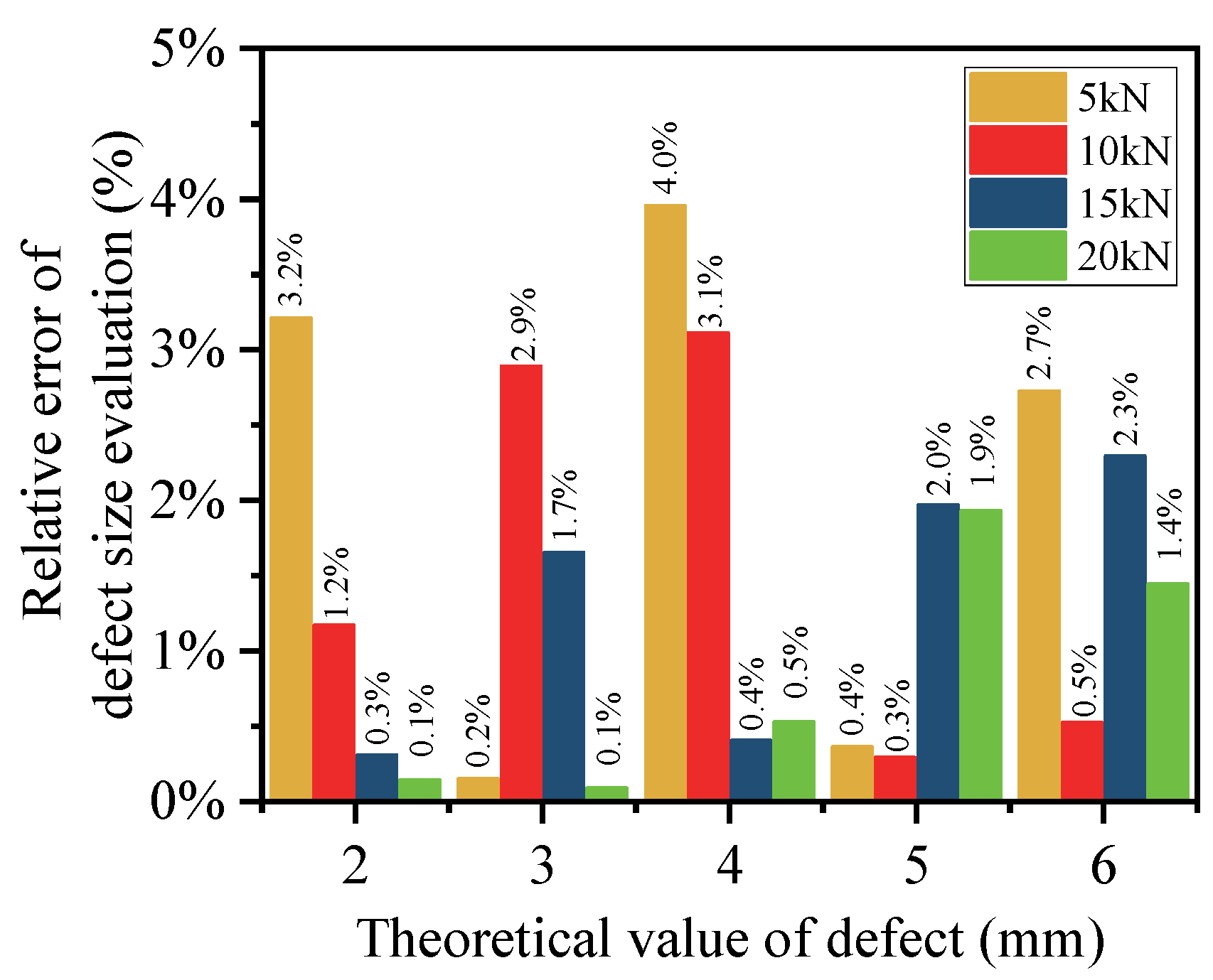
H are known. The error of the nonlinear fitting method in evaluating defect size is defined as follows:
where
ER is the relative error of defect size,
DT is the theoretical value of defect size, and
DE is the evaluation value of defect size. By substituting the measurement results, the evaluation error of defect size under different loads is shown in
Figure 19. The maximum relative error of defect size is 4.0%, indicating that this method could accurately evaluate defect size.
4. Conclusions
In this research, the variations in 3D MMS on the surface of specimen without a defect and with a circular hole defect were measured through tensile tests. The following conclusions were obtained:
(1) Hy of the 3D MMS contains the Y-directional position information of the defect, and the Y-directional position of the defect can be determined using Hy. The combined use of the three components of MMS is conducive to achieving accurate evaluation of defect location and size.
(2) The magnetic parameters ΔHx, ΔHy, and ΔHz increase with increasing load, but their peak–valley spacings, Δx, Δy, and Δz keep a constant value with increasing load. Different from the effects of load, the magnetic parameters ΔHx, ΔHy, and ΔHz and their corresponding peak–valley spacings Δx, Δy, and Δz increase with increasing defect size.
(3) The MMS gradient dH/dx can be used as a quantitative parameter to evaluate the equivalent stress σeqv along the loading direction.
(4) The Lissajous figure area generated from Hx and Hz of the MMS corresponds well to the defect size and stress, which can be used to quantitatively evaluate the defect size and stress, avoiding the deficiency of missing detection or misjudgment by using a single component.
(5) A nonlinear fitting equation based on MMS characteristic parameters, applied load and defect, size could accurately evaluate defect size with a relative evaluation error of 4%, providing an effective technical means for quantitatively evaluating defect size using magnetic memory detection technology for engineering applications.


