Analysis of Magnetization Dynamics in NiFe Thin Films with Growth-Induced Magnetic Anisotropies

Abstract

We have used angled magnetron sputter deposition with and without sample rotation to control the magnetic anisotropy in 20 nm NiFe films. Ferromagnetic resonance spectroscopy, with data analysis using a Bayesian approach, is used to extract material parameters relating to the magnetic anisotropy. When the sample is rotated during growth, only shape anisotropy is present, but when the sample is held fixed, a strong uniaxial anisotropy emerges with in-plane easy axis along the azimuthal direction of the incident atom flux. When the film is deposited in two steps, with an in-plane rotation of 90 degrees between steps, the two orthogonal induced in-plane easy-axes effectively cancel. The analysis approach enables precise and accurate determination of material parameters from ferromagnetic resonance measurements; this demonstrates the ability to precisely control both the direction and strength of uniaxial magnetic anisotropy, which is important in magnetic thin-film device applications.

1. Introduction

Magnetic anisotropies in ferromagnetic thin films are of central importance in magnetic data-storage, communications, and processing technologies [1]. The uniaxial magnetic anisotropy provides a means to stabilize magnetization along a pair of antiparallel directions that can be used to encode digital data; the detailed physical origins of such anisotropy is not well understood, despite extensive investigation of anisotropy induced by various methods [2,3,4,5,6].

A common approach to induce uniaxial magnetic anisotropy is oblique angled deposition, where the material source is positioned away from the substrate normal [7]. This has been employed with a variety of evaporation and sputter deposition techniques, resulting in microstructure where either crystal grains are elongated in the film plain along the direction from which the atom flux is incident [8], or at more extreme incidence angle in a ‘shadowing’ effect whereby columnar grains are tilted toward the incident flux direction [9]. This approach is convenient, since many deposition systems have confocal geometry, where rotation of the sample is used in an attempt to negate induced magnetic anisotropies [10].

Ferromagnetic resonance (FMR) spectroscopy techniques are frequently used to quantify magnetic anisotropies [11]. The GHz-frequency magnetization dynamics are commonly described as a damped-driven oscillator within the Landau–Lifshitz–Gilbert equation of motion,

$${\displaystyle \frac{d\mathbf{M}}{dt}}=-\gamma \mathbf{M}\times {\mathbf{H}}_{\mathrm{eff}}+{\displaystyle \frac{\alpha }{M_{\mathrm{s}}}}\mathbf{M}\times {\displaystyle \frac{d\mathbf{M}}{dt}}$$

for the macrospin magnetization $\mathbf{M}$, driven by an effective-field ${\mathbf{H}}_{\mathrm{eff}}$, and damped with a phenomenological Gilbert damping parameter $\alpha$. The gyromagnetic ratio, $\gamma =g{\mu }_{\mathrm{B}}/\hslash$, is related to the spectroscopic g-factor via the Bohr magneton and reduced Planck constant, and provides information on the spin–orbit coupling [12]. The effective field contains information on various magnetic material properties [13]; here, in particular, the various contributions to the magnetic anisotropy.

Under an excitation that balances the damping term, the relation between resonant frequency and applied field can be determined, yielding the well-known general Kittel equation,

$$F={\displaystyle \frac{\gamma }{2\pi }}\sqrt{\mathbf{B}·\mathbf{H}},$$

where $\mathbf{B}$ and $\mathbf{H}$ are the flux density and applied field at the resonance frequency, F. In the case of a thin-film with magnetization saturated along the in-plane applied field, the Kittel equation becomes

$$F={\displaystyle \frac{\gamma }{2\pi }}\sqrt{\left(H+H_{\mathrm{K}}\right)\left(H+H_{\mathrm{K}}+4\pi M_{\mathrm{eff}}\right)},$$

(1)

where H is the magnitude of the applied field at resonance and $H_{\mathrm{K}}$ is the component of the in-plane anisotropy field along the direction of the applied field and magnetization. The effective magnetization is related to the saturation magnetization $M_{\mathrm{S}}$, volume perpendicular magnetic anisotropy field $H_{\mathrm{k}}\perp$, surface magnetic anisotropy constant $K_{\mathrm{S}}$ and layer thickness $t_{\mathrm{FM}}$ by

$$4\pi M_{\mathrm{eff}}=4\pi M_{\mathrm{S}}-H_{\mathrm{k}}\perp +{\displaystyle \frac{2K_{\mathrm{S}}}{M_{\mathrm{S}}{t}_{\mathrm{FM}}}}.$$

(2)

If $H_{\mathrm{k}}\perp >0$ [$K_{\mathrm{S}}<0$] such that $M_{\mathrm{eff}}<M_{\mathrm{S}}$, then the volume [surface] anisotropy favours out-of-plane magnetization. In the case where the magnetization is saturated out of the plane of the sample by the applied field, the Kittel equation reduces to

$$F={\displaystyle \frac{\gamma }{2\pi }}\left(H-4\pi M_{\mathrm{eff}}\right),$$

(3)

which enables unambiguous separation and determination of the effective magnetization and spectroscopic g-factor, since only $\gamma$ determines the intercept; there is no such separation in the in-plane case (Equation (1)).

FMR measurements, thus, enable a breadth of information to be obtained on ferromagnetic thin-films, including magnetization, magnetic anisotropy, and spin–orbit coupling, and these can provide indirect information on the material microstructure. In this article, we use Ni₈₀Fe₂₀ thin films with magnetic anisotropies induced by angled sputter deposition as a model system to demonstrate the application of a unified Bayesian approach to modelling broadband FMR measurements. We show that this approach enables extraction of weak magnetic anisotropies and subtle variations in the material properties.

2. Materials and Methods

We deposited thin films of NiFe (Ni₈₁Fe₁₉—Permalloy) onto ∼8 mm $\times \sim$8 mm pieces cut from a Si(001) wafer substrate with a 100 nm thermal oxide coating, using an ultra-high vacuum magnetron sputter deposition system (Mantis Q-prep 500 (Thame, UK)) with a base pressure below $1\times {10}^{-8}$ Torr. Films were deposited from an alloy target of the stated composition under Ar working gas pressure of ∼1.5 mTorr, with deposition rates typically ∼0.25 Å/s. No seed or capping layers were used, and in all films the total NiFe thickness was nominally 20 nm. Film thicknesses were confirmed using X-ray reflectivity (Bruker D8 (Karlsruhe, Germany)), measured using Cu K-$\alpha$ radiation. X-ray reflectivity data are analysed using GenX software [14]. During deposition, samples can be rotated at up to 10 rpm, to prevent induced magnetic anisotropy and enhance large-area uniformity due to the confocal deposition geometry; the flux impinges on the sample from below, at an angle of 30 degrees from the sample normal. The sample can also be rotated and held static at any angle relative to the ‘home’ axis, defined here as having a specific side of the sample aligned parallel to the vacuum transfer arm into the deposition chamber. In epitaxial Fe growth on MgO, it has been found that a deposition angle of ∼30 degrees from the sample normal is the minimum at which magnetic anisotropy begins to be induced [8].

We discuss here three specific samples: for the first, the substrate is rotated at 10 rpm throughout the growth (‘rotated’); for the second, the the substrate is held static and aligned with the ‘home’ axis (‘static’); and for the third, the sample is deposited in two steps—for the first step, the sample is held static at an azimuthal angle 90 degrees from the ‘home’ axis, and for the second step, the sample is realigned with the ‘home’ axis. Return to the home axis is automatic, so this combination minimizes the exposure of the intermediate sublayer interface between deposition steps. Due to the ∼25 cm distance between target and substrate, the thickness variation across an individual sample (rotated or static) is around 1 %; the residual stray field from the magnetron sources at the sample position is weak, and we do not anticipate any field-induced anisotropy component.

Magnetization dynamics were measured using a broadband FMR spectrometer with a bandwidth up to 40 GHz. The sample is placed film-side against a coplanar waveguide (Signal Microwave, Tempe, AZ, USA) mounted between the poles of an electromagnet (GMW, San Carlos, CA, USA) to provide the applied magnetic field. The waveguide is excited using the amplitude-modulated output of a radio-frequency signal generator (Rohde & Schwarz, Munich, Germany). Modulation is typically at 5.275 kHz, with peak microwave power −5 dBm, and the waveguide is mounted such that the excitation field is always transverse to the applied magnetic field. The microwave absorption by the sample is obtained from the power output from the waveguide, using a power-detector diode (Krytar, Sunnyvale, CA, USA) and digital lock-in amplifier (Stanford Research Systems, Sunnyvale, CA, USA). In this case, the FMR signal can be described as a sum of coupled symmetric (absorption) and asymmetric (dispersion) Lorentzian lineshapes [15]; the measured power output from the waveguide is modelled as

$$P=-A{\displaystyle \frac{\Gamma }{2}}\left(cos\varphi {\displaystyle \frac{\Gamma /2}{{\Gamma }^2/4+{\left(H-H_{\mathrm{res}}\right)}^2}}-sin\varphi {\displaystyle \frac{H-H_{\mathrm{res}}}{{\Gamma }^2/4+{\left(H-H_{\mathrm{res}}\right)}^2}}\right),$$

(4)

superimposed on a (generally weak) locally quadratic background. Here, A is a collection of terms giving the signal amplitude, $\Gamma$ the full-width at half-maximum (FWHM) linewidth, H the applied magnetic field, $H_{\mathrm{res}}$ the resonance field, and $\varphi$ the mixing angle, which couples the absorption and dispersion components of the signal. Making measurements in this way requires an additional free parameter to fit the background (in field-modulated measurements [16], a locally linear background is often fitted), but has the benefits that modulation broadening of the absorption lineshape is absent, and that a higher modulation frequency can be used, allowing the applied field to be swept more quickly. Error-bars in the measured power are derived from a combination of the Johnson noise from the power-detector diode, and the amplifier input noise and digitization noise of the lockin-amplifier.

Measurements are made with the applied field either out of the plane of the sample, or in the sample plane. In all measurements here, the whole ∼8 mm $\times \sim$8 mm sample is used. For out-of-plane measurements the sample is separated from the waveguide by ∼70 $\mathsf{\mu }$m thick Polyimide tape to remove the radiative contribution to damping [17], and the maximum applied field is ∼20 kOe. In the case of in-plane measurements, the sample orientation relative to the applied magnetic field and excitation field is controlled by a precision rotation stage (Newport, Irvine, CA, USA), and the sample is mounted such that the film surface is ∼100 $\mathsf{\mu }$m from the waveguide; the maximum field in this configuration is ∼12 kOe. In all cases here, an in-plane sample angle of zero degrees corresponds to applied magnetic field parallel to the edge of the sample that is initially oriented along the transfer axis of the deposition system.

Analysis of FMR data are made using software based on the bumps fitting library [18] and its implementation of the ‘differential evolution with adaptive metropolis’ (dream) algorithm [19,20]. This uses a genetic algorithm to efficiently explore large-dimensional parameter spaces—it is more commonly used for fitting neutron reflectivity data [21]—to extract optimum parameter values, and a Bayesian approach to error analysis. Parameters are optimized by determining the maximum likelihood, which in the limit of Gaussian uncertainties is equivalent to minimizing ${\chi }^2$, and any ‘known’ parameter values and uncertainties can be included as ‘prior’ probability distributions. Parameter uncertainties are then evaluated from Markov-chain Monte Carlo sampling of the posterior probability distributions. Whilst this approach is more computationally costly than simpler fitting algorithms, it is beneficial in that we are able to obtain robust best fitting parameter values and uncertainties even when model parameters are strongly correlated; it is well-known that the spectrosocpic g-factor and effective magnetization are strongly (anti)correlated within the Kittel equation for in-plane magnetization—Equation (1), for example. The posterior probability distributions of the parameters enable clear visualization of any correlations and confirmation that the fit has successfully estimated the most likely set of parameter values, and appropriate uncertainties.

3. Results and Discussion

3.1. X-ray Reflectivity

We first briefly discuss structural characterization of the three films using X-ray reflectivity. Figure 1 shows reflectivity scans and best fits, along with the structural scattering length density (sSLD) model that produces the best fit. The reflectivity and fits for samples rotated during growth (lower), and held static during growth (upper), are shown in Figure 1a, and those for the sample deposited in two steps are shown in Figure 1c. The models describe the data well in each case, and the reflectivity measurements and sSLD [Figure 1b,d] appear broadly similar for all samples.

For the rotated sample, the sSLD that describes the data are a uniform NiFe layer with interface widths of around 0.8 nm, and a ∼1 nm surface oxide layer of lower density. The static sample is similar, but the density is slightly lower and the NiFe thickness slightly larger. The variation in thickness is compatible with the resolution of the quartz crystal deposition rate monitor in the deposition system, but may also indicate that the static film is slightly less dense but concomitantly thicker.

The sample deposited in two steps is best described by a model with two subtly different NiFe sublayers plus oxide surface layer; the lower sublayer has a slightly reduced density, similar to the static sample, and the upper sublayer has a density similar to the rotated sample. The total thickness is similar to the rotated sample, but the lower sublayer (90 degrees to ‘home’ axis) is ∼0.5 nm thicker than the upper (0 degrees) sublayer.

The lower density found for static deposition, and the first sublayer in two-step deposition, can be explained as a result of a slightly more porous grain structure due to grain shadowing during angled deposition [9]. In the two-step deposition, the 90 degree rotation between steps may partly disrupt the shadowing effect, perhaps explaining the slight increase in the density of the upper sub-layer.

3.2. FMR: Field-Swept Absorption

As an exemplar, Figure 2 shows angular dependent in-plane FMR measurements and analysis for the sample held static during deposition, expected to induce a uniaxial in-plane magnetic anisotropy. Figure 2a shows field-swept absorption measurements, made at a frequency of 10 GHz, measured at a range of angles from 0 degrees (top) to 360 degrees (bottom) in 10 degree steps. All data markers (red) are shown with error-bars, and all best fits (Equation (4)) have reduced-${\chi }^2$ in the range 0.9–2.2. A clear absorption peak is seen in all scans, the position of which varies in applied field with varying sample angle.

The upper panel of Figure 2b shows an example of a single field-swept absorption line. Data markers and error-bars are overlapped by the best fit (solid black line) and range of feasible solutions (solid red lines) sampled across posterior probability distributions (Markov chains); the lower panel shows normalized residuals (solid black points) and the range of normalized residuals corresponding to feasible solutions (red). The possible structure in the residuals, perhaps apparent close to where the absorption changes most rapidly, is due to the small noise in the field measurement and is not here indicative of additional absorption peaks [22]. The absorption (symmetric) and dispersion (asymmetric) components of the fitted lineshape—Equation (4)—are also shown.

Figure 2c shows parameter histograms of the posterior probability distributions from the fit in (b). The distributions are smooth, showing that sufficient Monte Carlo samples have been computed to assess the parameter uncertainties reliably, and the centre of the distribution matches the best-fitting solution—providing further confidence in fitting results. Heatmaps of parameter-pairs are shown in Figure 2d; for uncorrelated parameter pairs, the heatmap appears isotropic, whilst for strongly correlated parameter pairs, the heatmap appears as a diagonal line. The parameters describing the quadratic background are correlated, as expected, and, also as expected, the background is also somewhat correlated with both the absorption peak amplitude and FWHM linewidth. Thus, it is important to fit over a sufficiently large field range where the background is described well, in order to have confidence also in, for example, the extracted FWHM linewidth; but also fitting over a field range where the background remains locally quadratic. Since the parameter uncertainties are determined from the Monte Carlo sampling rather than from a covariance matrix, contributions to the reduced ${\chi }^2$ and normalized residual due to reasonable noise in the background generally have no significant impact. Finally, the mixing angle and resonance field are also somewhat correlated; the shape of the curve and position of the minimum in the model varies with the relative magnitude of the absorption and dispersion components.

Since the parameters in which we are typically primarily interested—the resonance field and FWHM linewidth—are reasonably strongly correlated with other parameters, this shows the importance of an analysis approach where the optimum values and uncertainties in correlated parameters can be estimated with confidence.

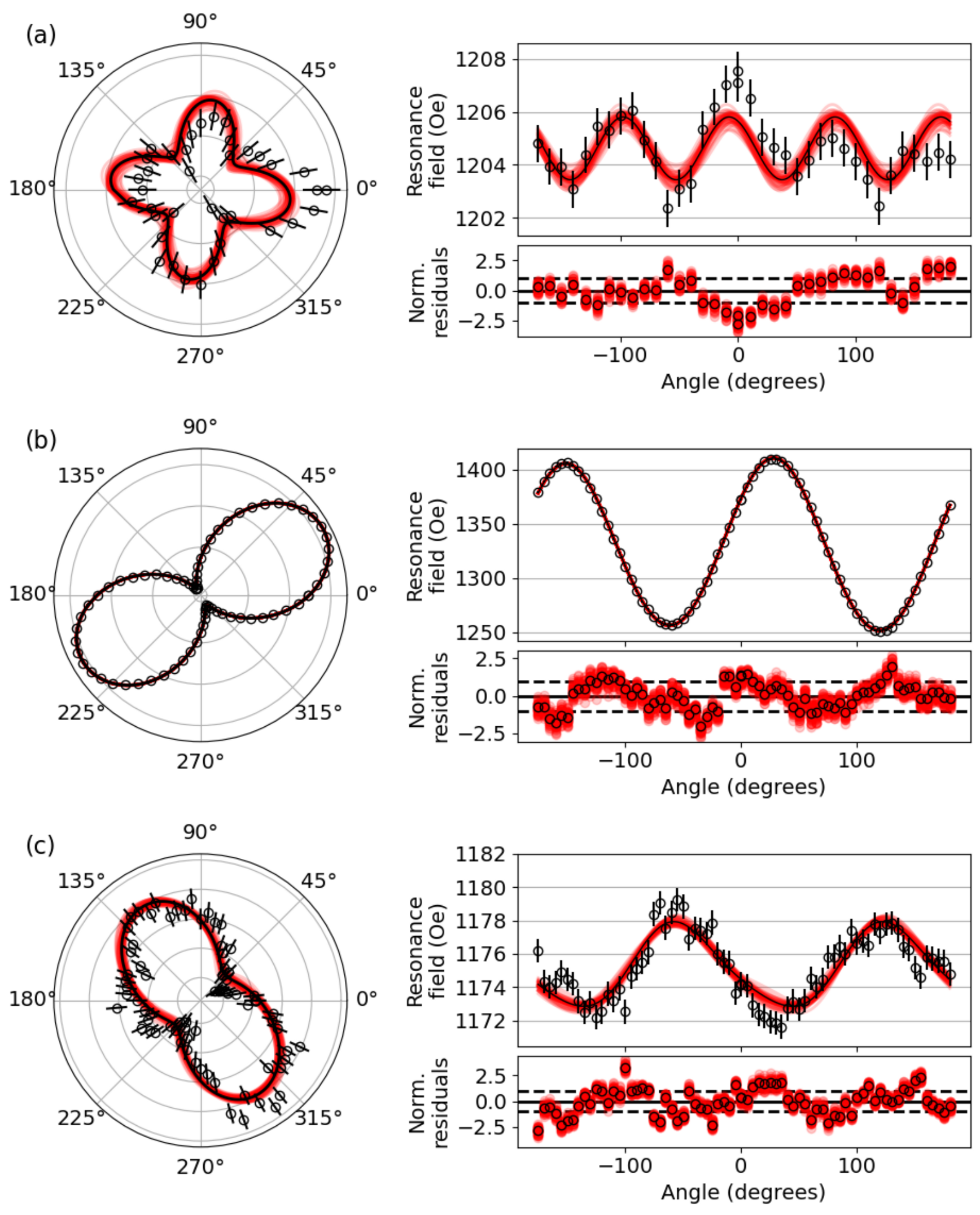
3.3. FMR: In-Plane Angular Dependence

Having extracted the angular dependence of the resonance field at fixed frequency, anisotropy fields and easy-axis orientations can be extracted from modelling. Figure 3 shows the angular dependence of the resonance field at frequency 10 GHz for the three samples discussed. In these plots, the solid black lines represent best fitting solutions, red lines represent feasible solutions sampled across Markov-chains, open points for normalized residuals represent those for the best fit, and red markers represent those for sampled feasible solutions. Error-bars in resonance field are obtained as a quadrature sum of the error in the fitted resonance field and the measurement uncertainty for an applied field of that value.

In Figure 3a, for the sample that is rotated during deposition, there is only a very weak dependence of the resonance field on in-plane sample orientation; here, the best fitting model (reduced-${\chi }^2=1.7$) is a four-fold in-plane magnetic anisotropy,

$$H_{\mathrm{res}}=H_0-H_{4}cos4\left(\theta -{\theta }_4\right),$$

where $H_0$ is the resonance field in the absence of anisotropy (if $H_{\mathrm{K}}=0$ in Equation (1)), $H_4$ the four-fold anisotropy field, and ${\theta }_4$ corresponds to the orientation of one of the four-fold easy-axes. We find an anisotropy field of $1.2\pm 0.2$ Oe oriented with easy axis at $37\pm 2$ degrees. Extracted results are given in

Table 1. Values for various contributions to the effective field obtained from angular dependent in-plane ferromagnetic resonance measurements made at frequency 10 GHz.

Sample	${\mathit{H}}_0$ (Oe)	${\mathit{H}}_{\mathbf{EB}}$ (Oe)	${\mathit{\theta }}_{\mathbf{EB}}$ (degrees)	${\mathit{H}}_{\mathbf{U}}$ (Oe)	${\mathit{\theta }}_{\mathbf{U}}$ (degrees)	${\mathit{H}}_4$ (Oe)	${\mathit{\theta }}_4$ (degrees)
Rotated	$1204.6\pm 0.1$	—	—	—	—	$1.2\pm 0.2$	$37\pm 2$
Static	$1329.5\pm 0.1$	$3.5\pm 0.2$	$166\pm 3$	$77.0\pm 0.2$	$118.7\pm 0.1$	$1.81\pm 0.15$	$70\pm 1$
Two-step	$1175.2\pm 0.1$	—	—	$2.5\pm 0.1$	$36.3\pm 0.14$	$0.34\pm 0.13$	$66\pm 6$

. Sputtered NiFe films deposited directly onto SiO₂ are polycrystalline with no preferred in-plane orientation; the weak four-fold anisotropy observed is not magnetocrystalline in origin, but is actually a shape-anisotropy due to the roughly square sample—with weak easy-axes along the sample diagonals. Quantifying these subtle anisotropies, which are not apparent in these films from hysteresis loop measurements, for example, shows the importance of being able to accurately and precisely extract resonance fields from FMR spectra by fitting.

Figure 3b shows the angular dependence extracted from the data in Figure 2 for the sample held static during deposition, developing an in-plane uniaxial magnetic anisotropy. The best-fitting model (reduced-${\chi }^2=0.9$) includes contributions not only from a strong uniaxial anisotropy superimposed on a weak four-fold shape-anisotropy, but also a further weak unidirectional exchange-bias anisotropy, described by

$$H_{\mathrm{res}}=H_0-H_{4}cos4\left(\theta -{\theta }_4\right)-H_{\mathrm{U}}cos2\left(\theta -{\theta }_{\mathrm{U}}\right)-H_{\mathrm{EB}}cos\left(\theta -{\theta }_{\mathrm{EB}}\right),$$

(5)

where now $H_{\mathrm{U}}$ [$H_{\mathrm{EB}}$] is the uniaxial anisotropy [exchange-bias] field, and ${\theta }_{\mathrm{U}}$ [${\theta }_{\mathrm{EB}}$] is the orientation of an [the] easy-axis of the uniaxial anisotropy [exchange-bias] [23]. We do not observe a term with three-fold symmetry, which may be anticipated for anisotorpy induced by stray field from the magnetron sources during static deposition.

Whilst the four-fold and unidirectional anisotropies are weak in comparison to the uniaxial magnetic anisotropy, both are required to achieve a suitably good description of the data, and show up clearly as trends in the normalized residuals if omitted. The weak four-fold anisotropy is similar in strength to the rotated sample discussed previously, with the orientation of the easy axes due to the sample shape deviating somewhat from square. The weak unidirectional anisotropy likely results from oxidation primarily of Ni; NiO is an antiferromagnet with high ordering temperature. XRR shows an oxide layer at the surface, and there may also be a weaker oxidation at the SiO₂/NiFe interface, due to the absence of buffer/seed or capping layers. It is not immediately apparent why the exchange anisotropy axis might be oriented as it is—although it is close to one of the easy-axes of the shape anisotropy (${\theta }_{\mathrm{EB}}=166\pm 3$ degrees, ${\theta }_4\sim 160$ degrees), it is also close to the much stronger hard-axis of the uniaxial anisotropy.

The orientation of the uniaxial easy-axis corresponds to the direction from which the impinging atom flux arrives at the sample: there are six sputter sources, 60 degrees apart, and the NiFe film was grown from a source located 60 degrees away from the transfer axis ($\theta =0$). Depositing the sample with sputtered atom flux incident from an angle (60 degrees azimuthal, 30 degrees polar) from the sample induces uniaxial magnetic anisotropy.

Figure 3c shows the angular dependence for the sample deposited in two steps; for the first step, the incident atom flux is incident from an azimuthal direction 90 degrees from that for the static sample in frame (b), and for the second step, the sample has been rotated by 90 degrees in the azimuthal direction so as to be aligned with the static sample. As the two sublayers are nominally identical, we expect that the two induced uniaxial magnetic anisotropies in the two sublayers should cancel one another [3], and a single resonance is observed at all fields since the two nominally identical sub-layers are strongly exchange coupled together at the interface [24]. The best-fitting model (reduced-${\chi }^2=1.7$) for the angular dependence includes contributions from a uniaxial anisotropy superimposed on a weak four-fold shape-anisotropy; as Equation (5), but without the final term in $H_{\mathrm{EB}}$. We again do not observe a term with six-fold symmetry, induced by stray field from the magnetron sources during two-step static deposition.

The four-fold anisotropy field is slightly weaker than in the other samples, $0.34\pm 0.13$ Oe, and again the orientation is due to the sample being cut somewhat off-square. The uniaxial anisotropy field is also far weaker than that in the static sample, now only $2.5\pm 0.1$ Oe; orthogonal (presumably) strong uniaxial anisotropies in the two sub-layers result in a weak overall uniaxial anisotropy due to slight mismatch in the magnetic moments of the two sublayers [3,24], due to the magnetization and/or thickness being slightly mismatched. The single peaks in the in-plane FMR spectra (Figure 4) indicate that the difference in density between the two sublayers, found in XRR measurements, does not result in a resolvable difference in magnetization; coupled layers of significantly different magnetization result in clear multiple resonance peaks [22,25]. However, the small difference in sublayer thickness (∼9.8 nm for the lower sublayer vs. ∼9.3 nm for the upper sublayer) means that the magnetic moment of the lower sublayer ‘dominates’. The net uniaxial magnetic anisotropy, with anisotorpy field $2.5\pm 0.1$ Oe, is aligned orthogonal for that in the single-step static sample due to the different initial alignment of these two samples. This demonstrates that multi-step angled deposition can be used to tailor the direction and magnitude of uniaxial magnetic anisotropies in thin magnetic films.

Despite the fact that correlations between parameters in these models for the angular dependence of the anisotropy field are negligible, the Markov-chain Monte Carlo approach remains useful here, since it provides further confidence in the fitted parameters, and illustrates the range of feasible solutions. In Figure 3, unambiguously resolving the small variations in resonance field in frames (a) and (c), and the subtle additional effects in frame (b) require robust fitting of the resonance lineshapes to extract the resonance field precisely and accurately.

3.4. FMR: Frequency Dependence

From Table 1, we see that the $H_0$ value for the single-step static sample with uniaxial anisotropy is somewhat higher than for the other samples; this suggests that the effective magnetization or g-factor for this NiFe film is somewhat smaller than those for the other films. The frequency dependence of the resonance field can be fitted with the appropriate form of the Kittel equation, and Equations (1) and (3) to determine these properties.

3.4.1. Out-of-Plane Field

The effective magnetization and (out-of-plane) g-factor are best determined from out-of-plane measurements, since in the Kittel equation for out-of-plane magnetization, these two properties are less strongly correlated than in the in-plane case. Whilst the g-factor may be anisotropic (more generally it is a tensor), the effective magnetization can be most accurately determined from out-of-plane measurements. We note also that the inhomogeneous linewidth and Gilbert damping are also best determined from the frequency-dependent linewidth made in the in out-of-plane geometry, since the confounding two-magnon scattering mechanism is inactive in this geometry [26,27,28]; the probability distribution obtained for the out-of-plane g-factor from fitting the Kittel equation is used as a Bayesian prior when calculating the Gilbert damping—however, we do not discuss the linewidth or damping here.

Figure 5 shows example out-of-plane frequency-dependent FMR measurement for the static sample. The signal to-noise is lower than for in-plane measurements since the larger field required to saturate the magnetization out-of-plane results in a smaller precession cone angle and so far lower power absorption. The data are again modelled using Equation (4), as for the in-plane data.

The frequency dependence of the out-of-plane resonance field for the rotated sample is shown in Figure 6a, along with the best-fit to the linear Kittel relation (Equation (3)). Normalized residuals are shown in the right panel, since the dominant source of error is in the fitted resonance field values. Fitted values from out-of-plane Kittel fitting are given in

Table 2. Ferromagnetic resonance results from fitting frequency dependence of resonance field for out-of-plane (OOP) and in-plane (IP) field measurements. In fitting the out-of-plane Kittel model, the parameters are less strongly coupled than in the in-plane case, so the out-of-plane value for $4\pi M_{\mathrm{eff}}$ is used as a Bayesian prior in the fitting to determine the component of the in-plane g-factor.

Sample	OOP $4\mathit{\pi }{\mathit{M}}_{\mathbf{eff}}$	OOP g-Factor	IP $4\mathit{\pi }{\mathit{M}}_{\mathbf{eff}}$	IP g-Factor
	(G)		(G)	0 Degrees	90 Degrees
Rotated	$9190\pm 10$	$2.243\pm 0.005$	$9180\pm 10$	$2.022\pm 0.002$	–
Static	$8010\pm 10$	$2.179\pm 0.005$	$8025\pm 6$	$2.014\pm 0.001$	$2.022\pm 0.001$
Two-step	$9430\pm 10$	$2.283\pm 0.005$	$9417\pm 10$	$2.035\pm 0.002$	–

. The extracted effective magnetization for the NiFe films are consistent with other values extracted by out-of-plane FMR measurements on similar NiFe films [29]. The out-of-plane g-factor is slightly larger, likely due to the films here being thinner; symmetry breaking at the surfaces has a more significant impact on the g-factor here [30,31].

For the single-step sample, with strong in-plane uniaxial anisotropy, both the effective magnetization and g-factor are somewhat smaller than for the other samples. The two-step sample has slightly higher effective magnetization and g-factor than the rotated sample. These are consistent with the $H_0$ values from in-plane rotation measurements (Table 1).

Out-of-plane FMR allows us to obtain a robust measure of the effective magnetization. Using the Bayesian data analysis approach, we can use the posterior distribution of plausible values for the effective magnetization extracted from out-of-plane FMR as a prior probability distribution input into the model for the frequency dependence of the in-plane magnetization; reducing the number of effective fitting parameters while also including in the analysis the distribution describing the uncertainty in this parameter.

3.4.2. In-Plane Field

The frequency dependence of the in-plane resonance field is described by Equation (1). This contains three parameters: the effective magnetization, the appropriate component of the g-factor, and the anisotropy field. As described in the previous section, the probability distribution of effective magnetization values has already been determined from fitting the frequency dependence of resonance field from out-of-plane measurements. The anisotropy field, $H_{\mathrm{k}}=H_{\mathrm{res}}-H_0$ is also known from fitting the in-plane angular dependence, both in appropriate functional form and parameter probability distributions.

The more common approach is to fit Equation (1) and then compare the extracted fitting parameters—effective magnetization, g-factor and anisotropy field—with those from other measurements; the strong correlation between g-factor and effective magnetization in this expression produces a parameter space with minima shaped such that reliable extraction of uncertainties from an estimate of the covariance matrix can be inaccurate. Instead, here we insert the appropriate expression for the angular dependence of $H_{\mathrm{K}}$ into Equation (1), and provide distributions of values for all parameters other than the g-factor component as Bayesian priors. Thus, we essentially extract only a single parameter, the in-plane g-factor component along a specific direction (here 0 degrees, for convenience), but properly including the distributions of values for all of the other parameters determined previously. (In fact, the effective magnetization is also allowed to vary from the value extracted from out-of-plane measurements, but the fitted value is seeded by the Bayesian prior, and the prior and posterior probability distributions should remain consistent).

Table 2 shows the results of such fitting for our three samples. For the rotated and two-step samples (not shown), we assess the g-factor only along one axis, anticipating anisotropy in the in-plane g-factor to be negligible. That the in-plane g-factor (components) values do not generally match the out-of-plane values demonstrates that the common assumption of an isotropic g-factor is an oversimplification.

For the static sample, with strong in-plane uniaxial magnetic anisotropy, we have also simultaneously fitted datasets along two orthogonal directions, with all parameters other than the g-factor shared—i.e., effective magnetization and the various terms comprising $H_{\mathrm{K}}$. The best simultaneous fits, shown in Figure 6b,c, give a reduced ${\chi }^2$ of 2.03. In all samples, we see that the effective magnetization remains consistent with that from the out-of-plane measurements. For the static sample, the in-plane g-factor is weakly anisotropic. We note that, in this example, we have arbitrarily chosen orthogonal directions parallel the the substrate sides rather than the anisotropy axes of the sample; with more measurements, the anisotropy in in-plane g-factor can be mapped out. However, the aim here is to demonstrate the sensitivity of the fitting approach in determining anisotropy in the g-factor.

The fact that it is possible to model both angular variation in the Kittel behaviour and the angular behaviour of the resonance field with a single set of common parameters provides further confidence that all significant contributions to the in-plane anisotropy have been adequately accounted for in the modelling.

The origin of the reduced magnetization in the static sample is unclear. It may be that a more porous grain structure formed by grain shadowing during angled deposition results in easier transit of atmospheric oxygen along, and incorporation into, grain-boundaries. This may also explain the weak exchange-bias observed in the angular dependence measurements. However, we might also expect a similar effect in the two-step sample; whist the columnar grain structure is disrupted at the point where the sample is rotated, such oxygen migrations should still be possible. However, the two-step sample has a higher effective magnetization that the rotated sample, so this seems unlikely. Alternatively, the angled deposition may cause an increase in interfacial (or volume) perpendicular magnetic anisotropy, acting to reduce the effective magnetization (Equation (2)); again, it is unclear why the two-stage deposition should result in the opposite effect, since both sublayers are also deposited in a similar manner. Further investigation is required to understand this, but the evidence from FMR measurements is clear, and supports with what can also be observed from X-ray reflectivity.

4. Conclusions

We have used the uniaxial magnetic anisotropy that can be induced during growth due to incident atom flux at a fixed angle to the sample normal as an example to demonstrate analysis of ferromagnetic resonance spectroscopy data using a Bayesian approach based on the bumps fitting and analysis library. Using this approach to model the field-swept absorption lineshape provides robust estimates of the resonance field and linewidth, despite correlations with other parameters in the model. Fitting the angular dependence of the accurately and precisely extracted resonance field allows determination of the relevant anisotropy terms that should be included in describing the sample, even in cases where the anisotropy is weak. The frequency-dependence of resonance field in the out-of-plane geometry requires larger applied magnetic field, but provides unambiguous determination of the effective magnetization and out-of-plane component of the spectroscopic g-factor. Values of effective magnetization and contributions to the angular-dependent in-plane effective field are then used as Bayesian priors when modelling the frequency-dependence of the in-plane resonance field with field applied at arbitrary angles in the sample plane. This enables the anisotropy in the in-plane g-factor to be extracted; this is important in understanding phenomena related to structural symmetry breaking and spin–orbit coupling in magnetic thin-film multilayers and devices. We have also shown that we are able to control the direction, and magnitude, of the induced uniaxial magnetic anisotropy by controlling the multi-stage growth of thin-films by angled deposition, which can be broadly useful in magnetic thin film device applications.

References

1. Hirohata, A.; Yamada, K.; Nakatani, Y.; Prejbeanu, I.L.; Diény, B.; Pirro, P.; Hillebrands, B. Review on spintronics: Principles and device applications. J. Magn. Magn. Mater. 2020, 509, 166711. [Google Scholar] [CrossRef]
2. Blois, M.S., Jr. Preparation of Thin Magnetic Films and Their Properties. J. Appl. Phys. 1955, 26, 975–980. [Google Scholar] [CrossRef]
3. Suits, F. Bilayer Permalloy films grown in orthogonal applied fields. IEEE Trans. Magn. 1990, 26, 2353–2355. [Google Scholar] [CrossRef]
4. Hindmarch, A.T.; Kinane, C.J.; MacKenzie, M.; Chapman, J.N.; Henini, M.; Taylor, D.; Arena, D.A.; Dvorak, J.; Hickey, B.J.; Marrows, C.H. Interface induced uniaxial magnetic anisotropy in amorphous CoFeB films on AlGaAs(001). Phys. Rev. Lett. 2008, 100, 117201. [Google Scholar] [CrossRef]
5. Hindmarch, A.T.; Rushforth, A.W.; Campion, R.P.; Marrows, C.H.; Gallagher, B.L. Origin of in-plane uniaxial magnetic anisotropy in CoFeB amorphous ferromagnetic thin films. Phys. Rev. B 2011, 83, 212404. [Google Scholar] [CrossRef]
6. Seeger, R.L.; Millo, F.; Mouhoub, A.; de Loubens, G.; Solignac, A.; Devolder, T. Inducing or suppressing the anisotropy in multilayers based on CoFeB. Phys. Rev. Mater. 2023, 7, 054409. [Google Scholar] [CrossRef]
7. Atkinson, D.; Searle, S.; Jefferies, M.; Levy, J.; Cramman, H. Controlling Anisotropy of NiFe Thin Films During Deposition for Device Applications. Sens. Lett. 2013, 11, 13–20. [Google Scholar] [CrossRef]
8. Zhan, Q.f.; Van Haesendonck, C.; Vandezande, S.; Temst, K. Surface morphology and magnetic anisotropy of Fe/MgO(001) films deposited at oblique incidence. Appl. Phys. Lett. 2009, 94, 042504. [Google Scholar] [CrossRef]
9. Frisk, A.; Achinuq, B.; Newman, D.G.; Heppell, E.; Dąbrowski, M.; Hicken, R.J.; van der Laan, G.; Hesjedal, T. Controlling In-Plane Magnetic Anisotropy of Co Films on MgO Substrates using Glancing Angle Deposition. Phys. Status Solidi A 2023, 220, 2300010. [Google Scholar] [CrossRef]
10. Chowdhury, N.; Bedanta, S. Controlling the anisotropy and domain structure with oblique deposition and substrate rotation. AIP Adv. 2014, 4, 027104. [Google Scholar] [CrossRef]
11. Farle, M. Ferromagnetic resonance of ultrathin metallic layers. Rep. Prog. Phys. 1998, 61, 755. [Google Scholar] [CrossRef]
12. Shaw, J.M.; Knut, R.; Armstrong, A.; Bhandary, S.; Kvashnin, Y.; Thonig, D.; Delczeg-Czirjak, E.K.; Karis, O.; Silva, T.J.; Weschke, E.; et al. Quantifying Spin-Mixed States in Ferromagnets. Phys. Rev. Lett. 2021, 127, 207201. [Google Scholar] [CrossRef]
13. Azzawi, S.; Hindmarch, A.T.; Atkinson, D. Magnetic damping phenomena in ferromagnetic thin-films and multilayers. J. Phys. Appl. Phys. 2017, 50, 473001. [Google Scholar] [CrossRef]
14. Glavic, A.; Björck, M. GenX 3: The latest generation of an established tool. J. Appl. Crystallogr. 2022, 55, 1063–1071. [Google Scholar] [CrossRef]
15. Montoya, E.; McKinnon, T.; Zamani, A.; Girt, E.; Heinrich, B. Broadband ferromagnetic resonance system and methods for ultrathin magnetic films. J. Magn. Magn. Mater. 2014, 356, 12–20. [Google Scholar] [CrossRef]
16. Swindells, C.; Hindmarch, A.T.; Gallant, A.J.; Atkinson, D. Spin current propagation through ultra-thin insulating layers in multilayered ferromagnetic systems. Appl. Phys. Lett. 2020, 116, 042403. [Google Scholar] [CrossRef]
17. Edwards, E.R.; Nembach, H.T.; Shaw, J.M. Co25Fe75 Thin Films with Ultralow Total Damping of Ferromagnetic Resonance. Phys. Rev. Appl. 2019, 11, 054036. [Google Scholar] [CrossRef]
18. Kienzle, P.; Krycka, J.; Patel, N.; Sahin, I. Bumps (Version 0.9.1) [Computer Software]; University of Maryland: College Park, MD, USA. Available online: https://github.com/bumps/bumps (accessed on 16 October 2024).
19. Vrugt, J.A.; ter Braak, C.J.F.; Clark, M.P.; Hyman, J.M.; Robinson, B.A. Treatment of input uncertainty in hydrologic modeling: Doing hydrology backward with Markov chain Monte Carlo simulation. Water Resour. Res. 2008, 44, W00B09. [Google Scholar] [CrossRef]
20. Vrugt, J.A.; ter Braak, C.J.F.; Gupta, H.V.; Robinson, B.A. Equifinality of formal (DREAM) and informal (GLUE) Bayesian approaches in hydrologic modeling? Stoch. Environ. Res. Risk Assess. 2009, 23, 1011. [Google Scholar] [CrossRef]
21. Kienzle, P.; Krycka, J.; Patel, N.; Sahin, I. Refl1D [Computer Software]; University of Maryland: College Park, MD, USA. Available online: https://github.com/reflectometry/refl1d (accessed on 16 October 2024).
22. Omelchenko, P.; Girt, E.; Heinrich, B. Test of spin pumping into proximity-polarized Pt by in-phase and out-of-phase pumping in Py/Pt/Py. Phys. Rev. B 2019, 100, 144418. [Google Scholar] [CrossRef]
23. Chechenin, N.G.; Dzhun, I.O.; Babaytsev, G.V.; Kozin, M.G.; Makunin, A.V.; Romashkina, I.L. FMR Damping in Thin Films with Exchange Bias. Magnetochemistry 2021, 7, 70. [Google Scholar] [CrossRef]
24. Layadi, A.; Artman, J. Ferromagnetic resonance in a coupled two-layer system. J. Magn. Magn. Mater. 1990, 92, 143–154. [Google Scholar] [CrossRef]
25. Stenning, G.B.G.; Shelford, L.R.; Cavill, S.A.; Hoffmann, F.; Haertinger, M.; Hesjedal, T.; Woltersdorf, G.; Bowden, G.J.; Gregory, S.A.; Back, C.H.; et al. Magnetization dynamics in an exchange-coupled NiFe/CoFe bilayer studied by x-ray detected ferromagnetic resonance. New J. Phys. 2015, 17, 013019. [Google Scholar] [CrossRef]
26. Arias, R.; Mills, D.L. Extrinsic contributions to the ferromagnetic resonance response of ultrathin films. Phys. Rev. B 1999, 60, 7395–7409. [Google Scholar] [CrossRef]
27. Lindner, J.; Barsukov, I.; Raeder, C.; Hassel, C.; Posth, O.; Meckenstock, R.; Landeros, P.; Mills, D.L. Two-magnon damping in thin films in case of canted magnetization: Theory versus experiment. Phys. Rev. B 2009, 80, 224421. [Google Scholar] [CrossRef]
28. Tokaç, M.; Kazan, S.; Özkal, B.; Al-jawfi, N.; Rameev, B.; Nicholson, B.; Hindmarch, A.T. Two Magnon Scattering Contribution to the Ferromagnetic Resonance Linewidth of Pt(Ir)/CoFeTaB/Ir(Pt) Thin Films. Appl. Magn. Reson. 2023, 54, 1053. [Google Scholar] [CrossRef]
29. Waring, H.J.; Li, Y.; Johansson, N.A.B.; Moutafis, C.; Vera-Marun, I.J.; Thomson, T. Exchange stiffness constant determination using multiple-mode FMR perpendicular standing spin waves. J. Appl. Phys. 2023, 133, 063901. [Google Scholar] [CrossRef]
30. Shaw, J.M.; Nembach, H.T.; Silva, T.J.; Boone, C.T. Precise determination of the spectroscopic g-factor by use of broadband ferromagnetic resonance spectroscopy. J. Appl. Phys. 2013, 114, 243906. [Google Scholar] [CrossRef]
31. Tokaç, M.; Bunyaev, S.A.; Kakazei, G.N.; Schmool, D.S.; Atkinson, D.; Hindmarch, A.T. Interfacial Structure Dependent Spin Mixing Conductance in Cobalt Thin Films. Phys. Rev. Lett. 2015, 115, 056601. [Google Scholar] [CrossRef]
Figure 1. (a) Measured X-ray reflectivity for single layer NiFe films where the sample is held static during growth (upper trace, blue) and rotated about the sample normal at 10 rpm (lower trace, red). Best fitting models of the sample structure are shown as the solid lines through the data, which are generated from the structural scattering-length densities (sSLD) shown in (b). (c,d) show the same for the case where the sample is deposited in two steps, with the sample static during each step, but rotated by 90 degrees between steps. A slight variation in density is apparent across the ‘interface’ corresponding to this break in deposition.
Magnetochemistry 10 00080 g001
Figure 2. (a) Measured transmitted power signals (black points) and respective fits (red lines) showing the in-plane angular-dependence of the ferromagnetic resonance field at 10 GHz for ‘static’ sample with growth-induced uniaxial in-plane magnetic anisotropy. (b) Exemplar background-subtracted transmitted power signal and lineshape fit for signal at θ = 30 degrees, corresponding roughly to magnetic field applied along the uniaxial hard-axis, and showing the absorption and dispersion components. Normalized residuals are shown in the lower panel. Best fit and residuals are shown in black, with red lines and markers showing the range of plausible solutions and associated residuals. (c) Histograms showing the posterior probability distributions of the parameters for the fit shown in (b). (d) Heatmaps of parameter pairs from the sampled posterior probability distributions showing correlation between pairs of fitting parameters.
Magnetochemistry 10 00080 g002
Figure 3. Angular dependence of the in-plane ferromagnetic resonance frequency for samples where (a) the sample is rotated during deposition, (b) the sample is held static during deposition, with the incident atom flux along an azimuthal angle corresponding to ∼120 degrees, and (c) the deposition is two-step, with the incident atom flux along ∼30 degrees in the first step and ∼120 degrees in the second step. Data and fits are shown with normalized residuals (below) on the right, and as polar plots on the left. The radial scale on the polar plots matches the vertical scale of the respective plots on the right. Solid black lines (open points in residual plots) correspond to the best fit (best fit residuals) and the broader overlapping red lines (filled points in the residual plots) show the range of feasible solutions (normalized residuals) sampled across posterior probability distributions.
Magnetochemistry 10 00080 g003
Figure 4. (a) Example ferromagnetic resonance measurement at 10 GHz for two-step sample, showing a single resonance peak, and resulting (b) parameter histograms and (c) correlation heatmaps. Best fit and residuals in (a) are shown in black, with red lines and markers showing the range of plausible solutions and associated residuals.
Magnetochemistry 10 00080 g004
Figure 5. (a) Measured power signals (black) and respective fits (red) for out-of-plane magnetization over a frequency range 5–20 GHz for the rotated sample. (b) Background-subtracted power signal and lineshape fit for signal at F = 10 GHz, showing the absorption and dispersion components. Normalized residuals are shown in the lower panel. Best fit and residuals are shown in black, with red lines and markers showing the range of plausible solutions and associated residuals. (c) Histograms showing the posterior probability distributions of the parameters for the fit shown in (b), and (d) heatmaps of the sampled posterior probability distributions showing correlation between pairs of fitting parameters.
Magnetochemistry 10 00080 g005
Figure 6. Kittel fits—frequency-dependence of the resonance field—for sample held static during deposition to induce uniaxial in-plane magnetic anisotropy. In (a), the applied field is perpendicular to the plane of the film, whereas in (b,c), the magnetic field is applied at a pair of arbitrary orthogonal directions in the sample plane, i.e., not specifically along uniaxial easy/hard axes, for example. On the right of each frame are normalized residuals; the line and markers are as in Figure 3.
Magnetochemistry 10 00080 g006