
Magnetohydrodynamic Analysis and Fast Calculation for Fractional Maxwell Fluid with Adjusted Dynamic Viscosity


Abstract
1. Introduction
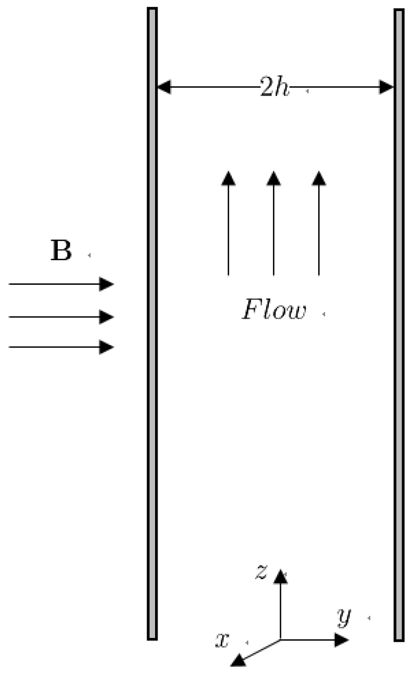
2. Mathematical Model
3. Numerical Method
3.1. Direct Method
3.2. Fast Method
4. Numerical Examples
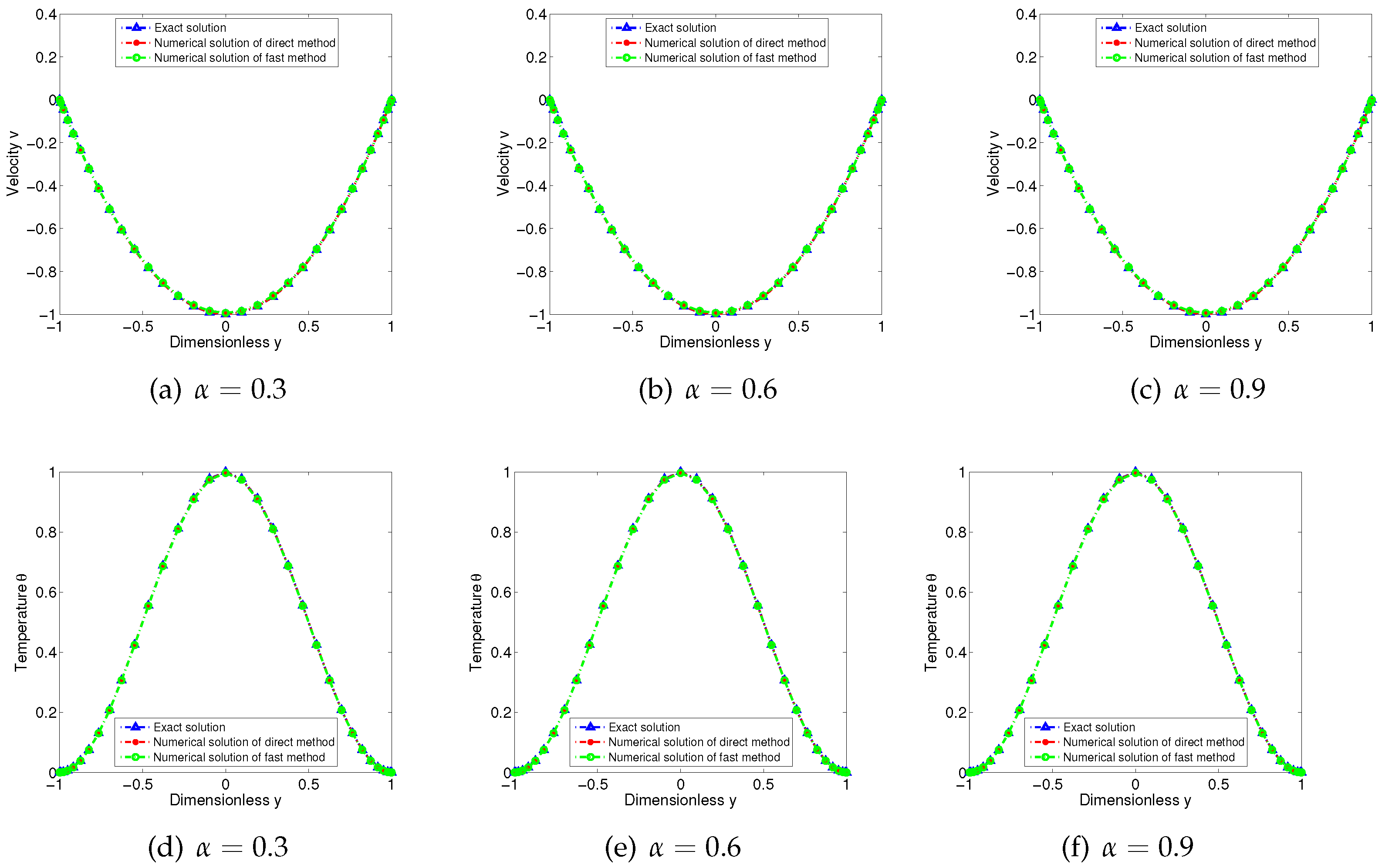
4.1. Example 1
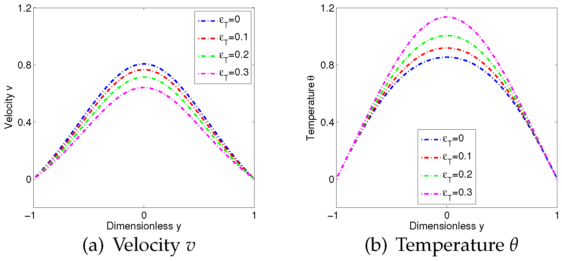
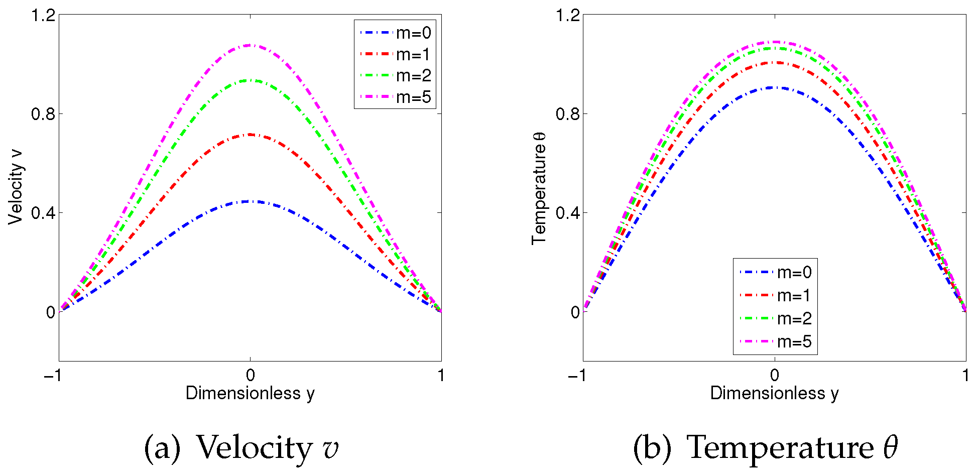
4.2. Example 2
5. Conclusions
Author Contributions
Funding
Data Availability Statement
Conflicts of Interest
References
- Pekmen, B.; Tezer-Sezgin, M. MHD flow and heat transfer in a lid-driven porous enclosure. Comput. Fluids 2014, 89, 191–199. [Google Scholar] [CrossRef]
- Cai, W.; Su, N.; He, X. MHD convective heat transfer with temperature-dependent viscosity and thermal conductivity: A numerical investigation. J. Appl. Math. Comput. 2016, 52, 305–321. [Google Scholar] [CrossRef]
- Vishalakshi, A.B.; Mahesh, R.; Mahabaleshwar, U.S.; Rao, A.K.; Pérez, L.M.; Laroze, D. MHD hybrid nanofluid flow over a stretching/shrinking sheet with skin friction: Effects of radiation and mass transpiration. Magnetochemistry 2023, 9, 118. [Google Scholar] [CrossRef]
- Ferdows, M.; Alam, J.; Murtaza, G.; Tzirtzilakis, E.E.; Sun, S. Biomagnetic flow with CoFe2O4 magnetic particles through an unsteady stretching/shrinking cylinder. Magnetochemistry 2022, 8, 27. [Google Scholar] [CrossRef]
- Liu, Y.; Liu, F.; Jiang, X. Numerical calculation and fast method for the magnetohydrodynamic flow and heat transfer of fractional Jeffrey fluid on a two-dimensional irregular convex domain. Comput. Math. Appl. 2023, 151, 473–490. [Google Scholar] [CrossRef]
- Zhang, L.; Lu, K.; Wang, G. An efficient numerical method based on Chelyshkov operation matrix for solving a type of time-space fractional reaction diffusion equation. J. Appl. Math. Comput. 2024, 70, 351–374. [Google Scholar] [CrossRef]
- Zheng, L.; Liu, Y.; Zhang, X. Slip effects on MHD flow of a generalized Oldroyd-B fluid with fractional derivative. Nonlinear Anal. Real World Appl. 2012, 13, 513–523. [Google Scholar] [CrossRef]
- Liu, Y.; Zheng, L.; Zhang, X. Unsteady MHD Couette flow of a generalized Oldroyd-B fluid with fractional derivative. Comput. Math. Appl. 2011, 61, 443–450. [Google Scholar] [CrossRef]
- Tassaddiq, A.; Khan, I.; Nisar, K.S.; Singh, J. MHD flow of a generalized Casson fluid with Newtonian heating: A fractional model with Mittag–Leffler memory. Alex. Eng. J. 2020, 59, 3049–3059. [Google Scholar] [CrossRef]
- Zhang, H.; Liu, F.; Phanikumar, M.S.; Meerschaert, M.M. A novel numerical method for the time variable fractional order mobile–immobile advection–dispersion model. Comput. Math. Appl. 2013, 66, 693–701. [Google Scholar] [CrossRef]
- Sun, H.; Chang, A.; Zhang, Y.; Chen, W. A review on variable-order fractional differential equations: Mathematical foundations, physical models, numerical methods and applications. Fract. Calc. Appl. Anal. 2019, 22, 27–59. [Google Scholar] [CrossRef]
- Yu, B. High-order efficient numerical method for solving a generalized fractional Oldroyd-B fluid model. J. Appl. Math. Comput. 2021, 66, 749–768. [Google Scholar] [CrossRef]
- Sheng, Z.; Liu, Y.; Li, Y. Finite element method combined with time graded meshes for the time-fractional coupled Burgers equations. J. Appl. Math. Comput. 2024, 70, 513–533. [Google Scholar] [CrossRef]
- Liu, F.; Zhuang, P.; Burrage, K. Numerical methods and analysis for a class of fractional advection–dispersion models. Comput. Math. Appl. 2012, 64, 2990–3007. [Google Scholar] [CrossRef]
- Jajarmi, A.; Ghanbari, B.; Baleanu, D. A new and efficient numerical method for the fractional modeling and optimal control of diabetes and tuberculosis co-existence. Chaos Interdiscip. J. Nonlinear Sci. 2019, 29, 093111. [Google Scholar] [CrossRef]
- Yavuz, M.; Sulaiman, T.A.; Usta, F.; Bulut, H. Analysis and numerical computations of the fractional regularized long-wave equation with damping term. Math. Methods Appl. Sci. 2021, 44, 7538–7555. [Google Scholar] [CrossRef]
- Wang, H.; Basu, T.S. A fast finite difference method for two-dimensional space-fractional diffusion equations. Siam J. Sci. Comput. 2012, 34, A2444–A2458. [Google Scholar] [CrossRef]
- Krishnarjuna, B.; Chandra, K.; Atreya, H.S. Accelerating NMR-Based Structural Studies of Proteins by Combining Amino Acid Selective Unlabeling and Fast NMR Methods. Magnetochemistry 2017, 4, 2. [Google Scholar] [CrossRef]
- Wang, K.; Wang, H. A fast characteristic finite difference method for fractional advection–diffusion equations. Adv. Water Resour. 2011, 34, 810–816. [Google Scholar] [CrossRef]
- Jiang, S.; Zhang, J.; Zhang, Q.; Zhang, Z. Fast evaluation of the Caputo fractional derivative and its applications to fractional diffusion equations. Commun. Comput. Phys. 2017, 21, 650–678. [Google Scholar] [CrossRef]
- Zhao, J.; Zheng, L.; Zhang, X.; Liu, F. Convection heat and mass transfer of fractional MHD Maxwell fluid in a porous medium with Soret and Dufour effects. Int. J. Heat Mass Transf. 2016, 103, 203–210. [Google Scholar] [CrossRef]
- Liu, Y.; Chi, X.; Xu, H.; Jiang, X. Fast method and convergence analysis for the magnetohydrodynamic flow and heat transfer of fractional Maxwell fluid. Appl. Math. Comput. 2022, 430, 127255. [Google Scholar] [CrossRef]
- Podlubny, I. Fractional Differential Equations; Academic Press: New York, NY, USA, 1999. [Google Scholar]
- Cowling, T. Magnetohydrodynamics; Interscience: New York, NY, USA, 1957. [Google Scholar]
- Wang, X.; Xu, H.; Qi, H. Transient magnetohydrodynamic flow and heat transfer of fractional Oldroyd-B fluids in a microchannel with slip boundary condition. Phys. Fluids 2020, 32, 103104. [Google Scholar] [CrossRef]
- Sun, Z.; Wu, X. A fully discrete difference scheme for a diffusion-wave system. Appl. Numer. Math. 2006, 56, 193–209. [Google Scholar] [CrossRef]
- Liu, L.; Yang, S.; Feng, L.; Xu, Q.; Zheng, L.; Liu, F. Memory dependent anomalous diffusion in comb structure under distributed order time fractional dual-phase-lag model. Int. J. Biomath. 2021, 14, 2150048. [Google Scholar] [CrossRef]
- Shen, J.; Tang, T.; Wang, L. Spectral Methods: Algorithms, Analysis and Applications; Springer: Berlin/Heidelberg, Germany, 2011. [Google Scholar]
- Liu, Y.; Zhang, H.; Jiang, X. Fast evaluation for magnetohydrodynamic flow and heat transfer of fractional Oldroyd-B fluids between parallel plates. Zamm-J. Appl. Math. Mech. Z. Angew. Math. Mech. 2021, 101, e202100042. [Google Scholar] [CrossRef]


| Error | Rate | Error | Rate | Error | Rate | ||
|---|---|---|---|---|---|---|---|
| v | 1/32 | - | - | - | |||
| 1/64 | 0.9650 | 0.9553 | 0.9595 | ||||
| 1/128 | 0.9822 | 0.9748 | 0.9771 | ||||
| 1/256 | 0.9907 | 0.9850 | 0.9854 | ||||
| 1/512 | 0.9951 | 0.9907 | 0.9897 | ||||
| 1/32 | - | - | - | ||||
| 1/64 | 1.0015 | 1.0089 | 1.0057 | ||||
| 1/128 | 0.9988 | 1.0032 | 1.0026 | ||||
| 1/256 | 0.9989 | 1.0018 | 1.0021 | ||||
| 1/512 | 0.9994 | 1.0013 | 1.0021 | ||||
Disclaimer/Publisher’s Note: The statements, opinions and data contained in all publications are solely those of the individual author(s) and contributor(s) and not of MDPI and/or the editor(s). MDPI and/or the editor(s) disclaim responsibility for any injury to people or property resulting from any ideas, methods, instructions or products referred to in the content. |
© 2024 by the authors. Licensee MDPI, Basel, Switzerland. This article is an open access article distributed under the terms and conditions of the Creative Commons Attribution (CC BY) license (https://creativecommons.org/licenses/by/4.0/).
Share and Cite
Liu, Y.; Jiang, M. Magnetohydrodynamic Analysis and Fast Calculation for Fractional Maxwell Fluid with Adjusted Dynamic Viscosity. Magnetochemistry 2024, 10, 72. https://doi.org/10.3390/magnetochemistry10100072
Liu Y, Jiang M. Magnetohydrodynamic Analysis and Fast Calculation for Fractional Maxwell Fluid with Adjusted Dynamic Viscosity. Magnetochemistry. 2024; 10(10):72. https://doi.org/10.3390/magnetochemistry10100072
Chicago/Turabian StyleLiu, Yi, and Mochen Jiang. 2024. "Magnetohydrodynamic Analysis and Fast Calculation for Fractional Maxwell Fluid with Adjusted Dynamic Viscosity" Magnetochemistry 10, no. 10: 72. https://doi.org/10.3390/magnetochemistry10100072
APA StyleLiu, Y., & Jiang, M. (2024). Magnetohydrodynamic Analysis and Fast Calculation for Fractional Maxwell Fluid with Adjusted Dynamic Viscosity. Magnetochemistry, 10(10), 72. https://doi.org/10.3390/magnetochemistry10100072