Interpretation of Hyperspectral Images Using Integrated Gradients to Detect Bruising in Lemons

Abstract

Lemons are a popular citrus fruit known for their medicinal and nutritional properties. However, fresh lemons are vulnerable to mechanical damage during transportation, with bruising being a common issue. Bruising reduces the fruit’s shelf life and increases the risk of bacterial and fungal contamination, leading to economic losses. Furthermore, discoloration typically occurs after 24 h, so it is crucial to detect bruised fruits promptly. This paper proposes a novel method for detecting bruising in lemons using hyperspectral imaging and integrated gradients. A dataset of hyperspectral images was captured in the wavelength range of 400–1100 nm for lemons that were sound and artificially bruised (8 and 16 h after bruising), with three distinct classes of images corresponding to these conditions. The dataset was divided into three subsets i.e., training (70%), validation (20%), and testing (10%). Spatial–spectral data were analyzed using three 3D-convolutional neural networks: ResNetV2, PreActResNet, and MobileNetV2 with parameter sizes of 242, 176, and 9, respectively. ResNetV2 achieved the highest classification accuracy of 92.85%, followed by PreActResNet at 85.71% and MobileNetV2 at 83.33%. Our results demonstrate that the proposed method effectively detects bruising in lemons by analyzing darker pixels in the images, subsequently confirming the presence of bruised areas through their spatial distribution and accumulation. Overall, this study highlights the potential of hyperspectral imaging and integrated gradients for detecting bruised fruits, which could help reduce food waste and economic losses.

1. Introduction

Lemon is a popular fruit owing to its high content of vitamin C, soluble fiber, calcium, pantothenic acid, and copper and its low-calorie count. It is known to aid in weight loss and reduce the risk of various diseases, such as kidney stones, cardiovascular ailments, and cancer [1]. However, fresh lemons are susceptible to mechanical damage during transportation, which can degrade their quality and decrease their market value [2]. Mechanical damage can accelerate the decay process of the whole lemon, leading to a significant increase in losses. Studies have shown that such losses can be as high as 51% of the total harvest [3]. Bruising is a type of mechanical damage that frequently occurs in produce during post-harvest operations, typically as a result of excessive loads. The bruised area of tissue experiences discoloration, which may not be readily apparent. However, this discoloration may become pronounced when the product is delivered to consumers or stored in a cooling facility [4]. The impact of bruising on fruits is noteworthy, as it diminishes their shelf life and increases the likelihood of bacterial and fungal contamination [5].

Bruising can be caused by the compression of the fruit against other objects, such as metallic surfaces of handling equipment, tree limbs, and other fruits [6,7,8]. Various studies have been conducted on bruising in different products such as pear [9], kiwifruits [10], tomato [11], and apples [12,13]). For instance, Gharaghani and Shahkoomahally [14] conducted a study on three apple cultivars and found that there was a significant and positive correlation between fruit size and bruising, while the correlations between bruising and fruit firmness, density, and dry matter were all significantly negative. It can be inferred from this study that firmer fruits, or those with a higher density and dry matter, tend to have more rigid cellular structures which can better withstand the impact forces that lead to bruising. Therefore, firmer, denser fruit, or those with a higher dry matter, are less vulnerable to bruising.

To ensure that a high quality of fruits is maintained during harvesting and handling, it is essential to identify and eliminate the root cause of bruising. However, given the inevitability of mechanical damage, efficient separation of damaged fruits is key to maintaining quality. Researchers have proposed various methods to detect and classify damaged fruits. For example, Yang et al. [15] reported on implementing polarization imaging (PI) technology to detect bruised nectarines. The authors collected images of 406 nectarines (280 bruised and 206 sound) and acquired PI at four polarization angles (0°, 45°, 90°, and 135°). The ResNet-18 integrated with ghost bottleneck was used to classify sound and bruised nectarines to classify fruits with an overall correct classification rate (CCR) of 97.69%. The average detection time for each fruit was 17.32 ms. NIR imaging technology combined with deep-learning methods has also been proposed to detect early-stage bruising. For instance, Xing et al. [16] acquired hyperspectral images of apple samples in the 900–2350 nm range and utilized three algorithms, viz., Yolov5s, Faster R-CNN, and Yolov3-Tiny, and reported a total accuracy of more than 99% at a detection speed of 6.8 ms per image. In another study, Li et al. [17] collected spectral data (397.5–1014 nm) of healthy peaches at 12, 24, 36, and 48 h after damage. The collected data were analyzed using a PCA model, which resulted in a CCR of 96.67%, 96.67%, 93.33%, and 83.33% for the respective time intervals. Yuan et al. [18] used SVM and PLS-DA to classify normal and bruised jujube fruit based on reflection and absorption spectra and reported the highest CCR of 88.9% using the PLS-DA model.

Moreover, hyperspectral imaging and a 1D-convolutional neural network were also utilized to detect bruises in apples, achieving an accuracy of 95.79% [19]. Similarly, hyperspectral imaging in the 450–1000 nm range was used with principal component analysis (PCA) to classify persimmons into healthy and bruised classes, and CCRs of 90% and 90.8%, respectively, were obtained [20]. In a substantial advancement, Mamat et al. [21] employed deep-learning models for the automatic annotation of a range of fruits. Utilizing a dataset of 100 images of oil fruit palm and 400 images of a variety of other fruits, their annotation technique proved successful in achieving high accuracy with average precisions of 98.7% for oil palm fruit and 99.5% for the other varieties. Similarly, a CNN-based seed classification system proposed by Gulzar et al. [22] demonstrated 99% accuracy during the training phase when classifying 14 commonly known seeds.

Prior studies have also explored the capabilities of hyperspectral imaging coupled with a few machine-learning models for bruise detection in lemons [23]. In this study, we aim to advance the state-of-the-art by exploring the efficacy of more advanced machine-learning models. Moreover, this study provides an interpretation of results via spatial analysis of hyperspectral images in damaged fruit. The main contributions of this work are outlined as follows:

• Proposing a novel method for detecting bruising in lemons using hyperspectral imaging and integrated gradients;
• Comparatively analyzing three different 3D-convolutional neural networks, viz. ResNetV2, PreActResNet, and MobileNetV2, for bruise detection in lemons;
• Establishing a robust and accurate method for early bruise detection in lemons that has the potential to reduce food waste and improve the overall quality of produce.

The advancements presented in this work offer a substantial stride forward in the field of post-harvest bruise detection and lay the groundwork for future studies on related topics. By leveraging cutting-edge technologies, the innovative methods and insights developed here pave the way for the broader application of hyperspectral imaging and advanced machine-learning models in bruise detection across a wide range of fruits and vegetables.

2. Materials and Methods

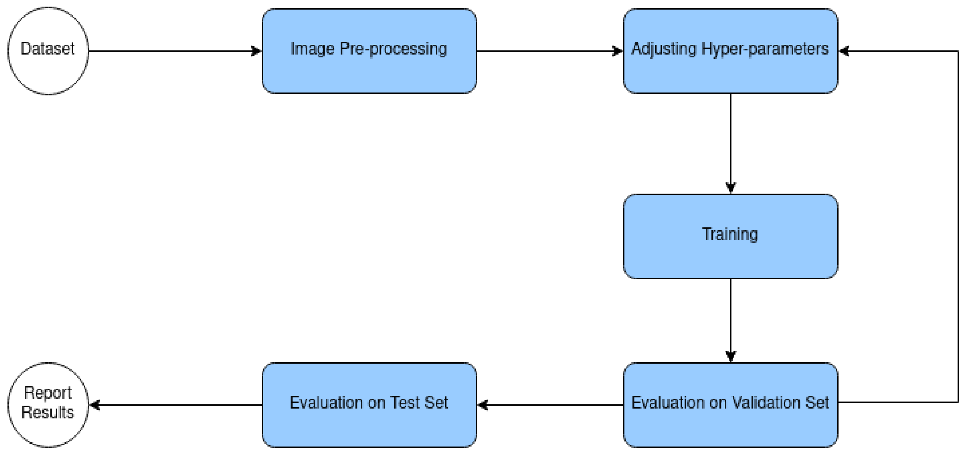
The proposed methodology for detecting bruising of lemon is illustrated in Figure 1, which depicts the flowchart of the process. The workflow begins with the initial data acquisition phase, where a total of 70 lemons were subjected to three different treatments resulting in 210 samples (see Section 2.1). This is followed by a pre-processing phase, in which the input dataset is resized and randomly divided into training, validation, and testing sets, with the division occurring in a 70%, 20%, and 10% ratio, respectively. This results in 147 training samples, 42 validation samples, and 21 testing samples. Next, the dataset is enriched by leveraging augmentation techniques to enhance model generalization. In this study, two specific types of augmentation were employed (see Section 2.3) on the training dataset, resulting in the number of training data increasing to three times the original size, i.e., 3 × 147 = 441. Following augmentation, the model undergoes an optimization process utilizing the augmented training set. In this stage, the model’s parameters are meticulously adjusted to maximize accuracy on the validation set. The validation set, distinct from the training set, serves to assess our model’s performance throughout the training phase. This validation allows one to fine tune the model’s hyperparameters and configurations based on the performance insights gained. Ultimately, the testing set is evaluated, which will be discussed in the results section.

2.1. Data Collection

First, a total of 70 hand-picked and intact lemons were carefully selected from a citrus garden located in Sari-Iran (36°34′4″ North, 53°3′31″ East). To ensure their safety during transportation, the fruits were covered with shock-absorbing foam and placed in a box in a single layer. Upon arrival at the laboratory, all fruits were labeled and imaged using a hyperspectral system (details are provided in Section 2.2). To induce artificial bruising, all samples were dropped from a height of 30 cm, which was determined via a trial-and-error process. This process involved dropping fruits from varying heights and assessing the resulting bruise severity, size, and appearance until a consistent and representative bruise was imparted to the fruit.

Hyperspectral data of all the samples were then acquired 8 and 16 h after the bruising occurred. Throughout the remainder of this manuscript, the terms classes A, B, and C refer to sound, 8 h, and 16 h after bruising, respectively. An example of such classification is illustrated in Figure 2.

2.2. Hardware Setup for Data Acquisition

Images were captured employing a pushbroom hyperspectral camera that incorporated an integrated scanner (Noor_imen_tajhiz Co., Kashan, Iran). The spectral range of the camera extended from 400 to 1100 nm, with a resolution of 2.5 nm. Each sample was individually placed on a flat, non-reflective surface, with the bruised side facing the camera at a distance of 1 m. The samples were placed without a holder to minimize background interference.

The process of image capture took approximately 2 min per sample. During this time, 400 lines were scanned to create a composite image of the entire sample in a pushbroom mode. The accuracy of the spatial resolution for an object at this distance is approximately 250 µm. This process was carried out for each sample individually to ensure a high level of detail and to prevent any potential interference between samples.

To illuminate the samples, a chamber equipped with two 20 W halogen lamps was used. The images were collected solely from the bruised side of the fruit, as the focus of this study was to analyze the progression of bruising over time. For each fruit, two images were captured, one at 8 h after bruising and another at 16 h after bruising, serving as replicates for each respective bruise stage.

2.3. Pre-Processing and 3D Structure of Samples

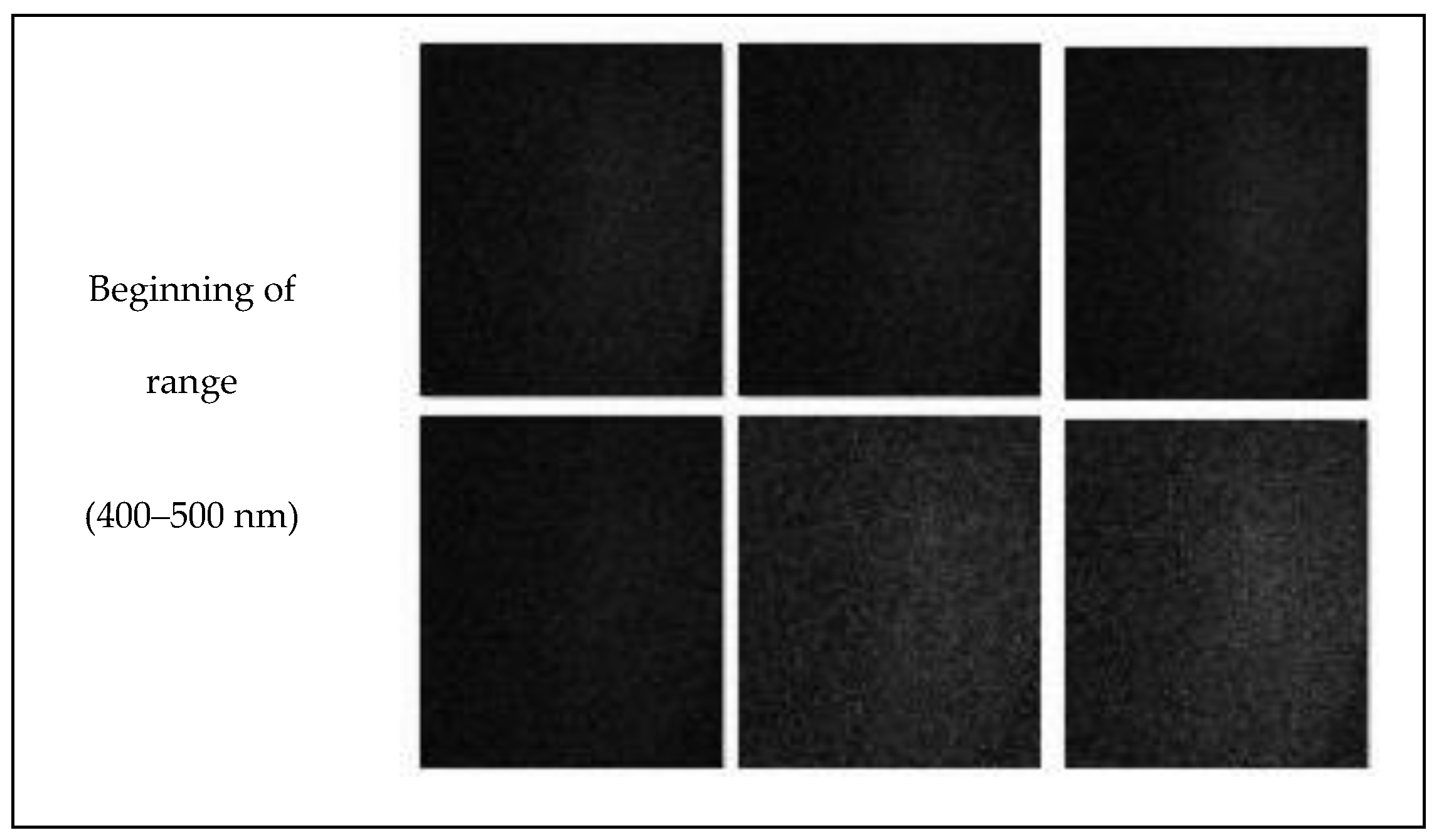
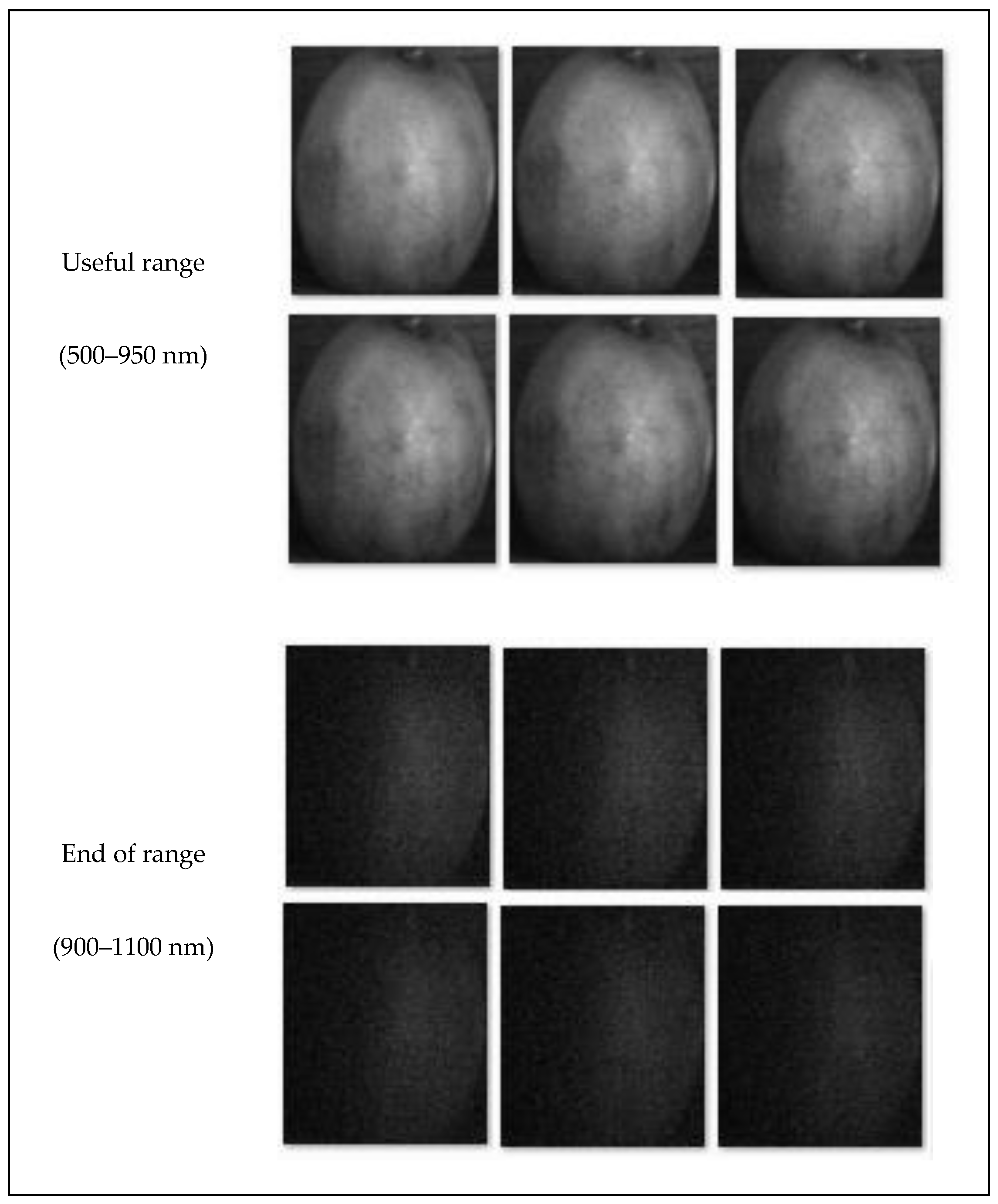
In hyperspectral imaging, the images generated are essentially three-dimensional, combining spatial (2D) and spectral (1D) information. As part of the analysis process, images at the extreme ends of the spectral range, suffering from a poor signal-to-noise ratio, were not considered in this study. Consequently, the focus remained on images within the 550–900 nm range (Figure 3).

The pre-processing phase involved refining this image set by removing noisy images and cropping image borders to exclude the background. This focused the analysis solely on the region of interest: the lemons (see Figure 3). This process yielded 174 spectral bands for each sample data, with each band representing a two-dimensional image of 160 × 120 pixels. Each pixel within these images corresponds to a spectrum of 174 values, reflecting the 174 spectral bands.

Subsequently, data augmentation techniques, namely RandomHorizontalFlip and Color Jitter, were applied to artificially expand the dataset and improve the model’s generalization ability. Data augmentation refers to a process that artificially amplifies the size of the training set by generating modified variants of the existing data. This could involve subtle alterations to the original data or leveraging deep learning to create new data instances. Finally, the labels (classes) were classified using the PyTorch framework and three 3D-CNN models, namely ResNetV2, MobileNetV2, and PreActResNet.

2.4. Three-Dimensional-Convolutional Classifiers

Three-dimensional-convolutional classifiers are deep-learning models that process input data using 3D-convolutional layers. These layers slide a small 3D kernel over the input volume to extract features. With this methodology, CNN layers mine spatial data from the images, resulting in the formation of coded feature matrices via feature extraction. Following this, the model applies densely connected layers of neural networks to formulate a projected label for the given classification.

The three 3D models used for classification had different training times and parameters size (

Table 1. Comparison of training times and parameter size of the proposed classifiers.

Model Name	Parameter Size (MB)	Train Time per Epoch (Seconds)
ResNetV2	242	25
PreActResNet	176	41
MobileNetV2	9	25

).

2.4.1. ResNetV2

ResNetV2 is a type of convolutional neural network architecture that belongs to the inception family. It encompasses residual connections, and its training involves more than a million images drawn from the ImageNet repository. The network architecture is extensive, with 164 layers, and boasts the competence to categorize images into 1000 distinct types of objects. These categories span a wide range, incorporating animals, keyboards, mice, and pencils, among others [24].

2.4.2. PreActResNet

PreActResNet is a variant of the original ResNet architecture with improved performance in image classification tasks. In PreActResNet [25], the activation layer is placed before the weight layer, unlike in the original ResNet architecture [25]. This modification has the potential to improve the performance of the network.

2.4.3. MobilNetV2

MobilNetV2 is a pre-trained model for image classification that is part of the MobileNet family of architectures. The network is designed to be lightweight and efficient, making it particularly suitable for applications on mobile devices or other resource-constrained environments. It has been trained on a large dataset (more than a million) of images and can classify them into 1000 object categories, such as animals, plants, vehicles, etc. The network is composed of multiple layers with a total depth of 53 [26].

2.5. Training, Testing, and Validation Sets

As mentioned before, the dataset was randomly split into training (70%), validation (20%), and testing (10%) sets [27]. This division serves different purposes in model development. The ‘external validation’ set is used during the model’s training phase to assess its performance and adjust the model’s parameters and hyperparameters accordingly. In contrast, the ‘testing’ set is used post-training to evaluate the model’s performance on unseen data, essentially simulating real-world scenarios. This distinction ensures that the model, while well-fitted to the training data, can also generalize to new, unseen data, thereby avoiding overfitting. The distribution of data in these sets is summarized in

Table 2. Samples quantity in the original dataset and the training/validation/testing sets.

Dataset	Number of Samples (Before Augmentation)	Class A (Sound)	Class B (8 h Passed Bruising)	Class C (16 h Passed Bruising)
Training	147	49	49	49
Validation	42	14	14	14
Testing	21	7	7	7

.

2.6. Evaluation Metrics

To ensure the robustness of our machine-learning models, a comprehensive array of evaluation metrics was employed to assess their performance and behavior throughout different stages of the modeling process.

2.6.1. Training and Validation Loss

Training and validation loss plots were integral to the performance evaluation process. These plots play a crucial role in visualizing the optimization of the model’s loss function, which is essentially a measure of error, during the training and validation stages. Throughout the training phase, the model learns by adjusting its internal parameters to minimize this error on the training dataset. For each iteration of the model’s training, the loss function is computed, and these values are captured in the training loss plot. The ideal trend we wish to observe is a consistent decrease in loss over time, indicating that the model is successfully learning from the data and improving its performance.

Subsequently, during the validation phase, the model’s ability to generalize its learning to new data is assessed. The model’s performance is evaluated on a validation dataset that was not used during training, and the validation loss plot captures these values. If the loss function shows a consistent decrease during this phase, it implies that the model has a good generalization ability, meaning it is capable of making accurate predictions on unseen data.

The analysis of training and validation loss plots provides deep insights into the model’s learning process. It can indicate whether the model is overfitting, where it performs well on the training data but poorly on new data, or underfitting, where it does not learn adequately from the training data. These plots, thus, guide model optimization.

2.6.2. Confusion Matrix

A confusion matrix, or error matrix, is a powerful tool for assessing model quality. Specifically in classification problems, the confusion matrix provides a detailed breakdown of how well the model predicts each class, comparing predicted labels against true labels.

2.6.3. Precision, Recall, and the Precision–Recall Curve

In classification problems, precision and recall are fundamental metrics. Precision is the fraction of true positives among all positive predictions and is calculated as Precision = TP/(TP + FP), where TP and FP refer to true positives and false positives, respectively. Recall, also known as sensitivity or true positive rate, is the fraction of true positives among all actual positives, calculated as Recall = TP/(TP + FN), where FN refers to a false negative.

The Precision–Recall Curve is a graphical representation of this trade off. This curve allows us to observe the variations in precision and recall as the decision threshold of the model changes, thereby shedding light on the model’s ability to balance between identifying as many positive samples as possible and keeping the prediction of false positives to a minimum.

2.6.4. Averaged Precision (AP)

AP summarizes a precision–recall curve as the weighted mean of precisions achieved at each threshold, with the increase in recall from the previous threshold used as the weight. The AP is calculated using the following formula: AP = Σ (R_n − R_n−1) P_n, where P_n and R_n are the precision and recall at the nth threshold.

2.6.5. Accuracy, F1-Score, and Micro-Averaged AP

Accuracy is a direct measure of the model’s performance, indicating the proportion of total samples that have been correctly classified by the model.

The F1-score is a harmonic mean of precision and recall, calculated as F1-score = 2 × (Precision × Recall)/(Precision + Recall), providing a balanced measure of the model’s performance. This metric is particularly useful in situations where both the identification of positive samples and the reduction in false positives are equally important [28,29,30].

Lastly, in scenarios involving multi-class classification, the micro-averaged AP offers a comprehensive performance evaluation. This metric considers each class’s precision and recall values and calculates an average that takes into account the total number of true positives, false positives, and false negatives across all classes. Essentially, micro-averaged AP provides a collective measure of a model’s precision and recall across all classes.

2.6.6. Receiver Operating Characteristic (ROC) Curves

In the context of binary classification problems, a ROC curve is a graphical representation that depicts the performance of a model. It is drawn by plotting the True Positive Rate (TPR), also known as recall or sensitivity, against the False Positive Rate (FPR) at various threshold settings.

The ROC curve encapsulates the trade off between sensitivity (or TPR) and specificity (1 − FPR). The area under the ROC curve, known as AUC-ROC, provides an aggregate measure of the model performance across all possible classification thresholds. An AUC-ROC score of 1 represents perfect classification, while a score of 0.5 implies that the model’s classification performance is no better than random guessing.

The ROC curves and their AUCs are valuable tools for evaluating and comparing the performance of classification models. They are especially useful in situations where the data may be imbalanced or when different misclassification costs are associated with the positive and negative classes. The ROC curve effectively illustrates these aspects, offering a comprehensive view of the model’s predictive ability across various thresholds.

3. Results and Discussion

3.1. The Final Structure of Classifiers

The hyperspectral images were processed by concatenating the spectra of each sample to create a 3D image inclusive of all spatial data of the images. The resulting input image size was 174 × 160 × 120 pixels with one input channel. During the training phase, the batch size was an important hyperparameter for the classifier. However, Google Colab’s GPU memory storage limitations presented obstacles. Furthermore, the 3D CNN models demanded more computational memory due to the increased volume of trainable parameters in their structure. To circumvent this problem, a batch size of 4, coupled with a gradient accumulation of two back propagations, was employed. Batch sizes were accumulated across two epochs prior to a single optimization step, effectively leading to a batch size of 8.

To fine tune the model, CrossEntropyLoss served as the optimization standard, and the Adadelta optimizer, featuring an exponential learning rate, was implemented to expedite convergence and add stochasticity during training. The initial learning rate was set at 0.1 and was exponentially diminished by a 0.95 factor.

The classifier’s concluding layer employed a Softmax layer to provide a probability prediction for each class. CrossEntropyLoss was utilized to determine the model’s error. The logits (probabilities) rendered by the Softmax layer were juxtaposed against the anticipated label vector. This vector was a one-hot vector with a single value at the index of the expected label and zeroes at other vector indices. Model parameters were then updated via backpropagation, which involved introducing an error on these logits.

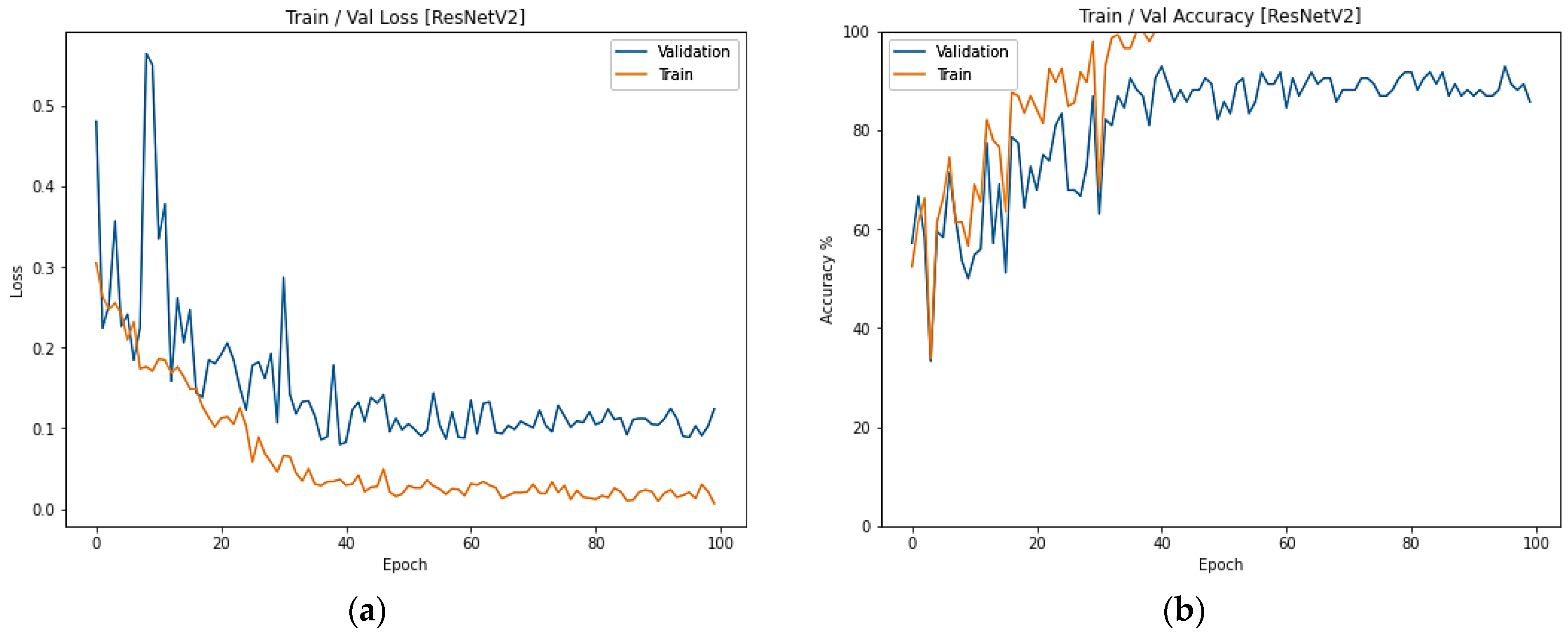
3.2. The Behavior of Different Classifiers in the Training and Validation Phases

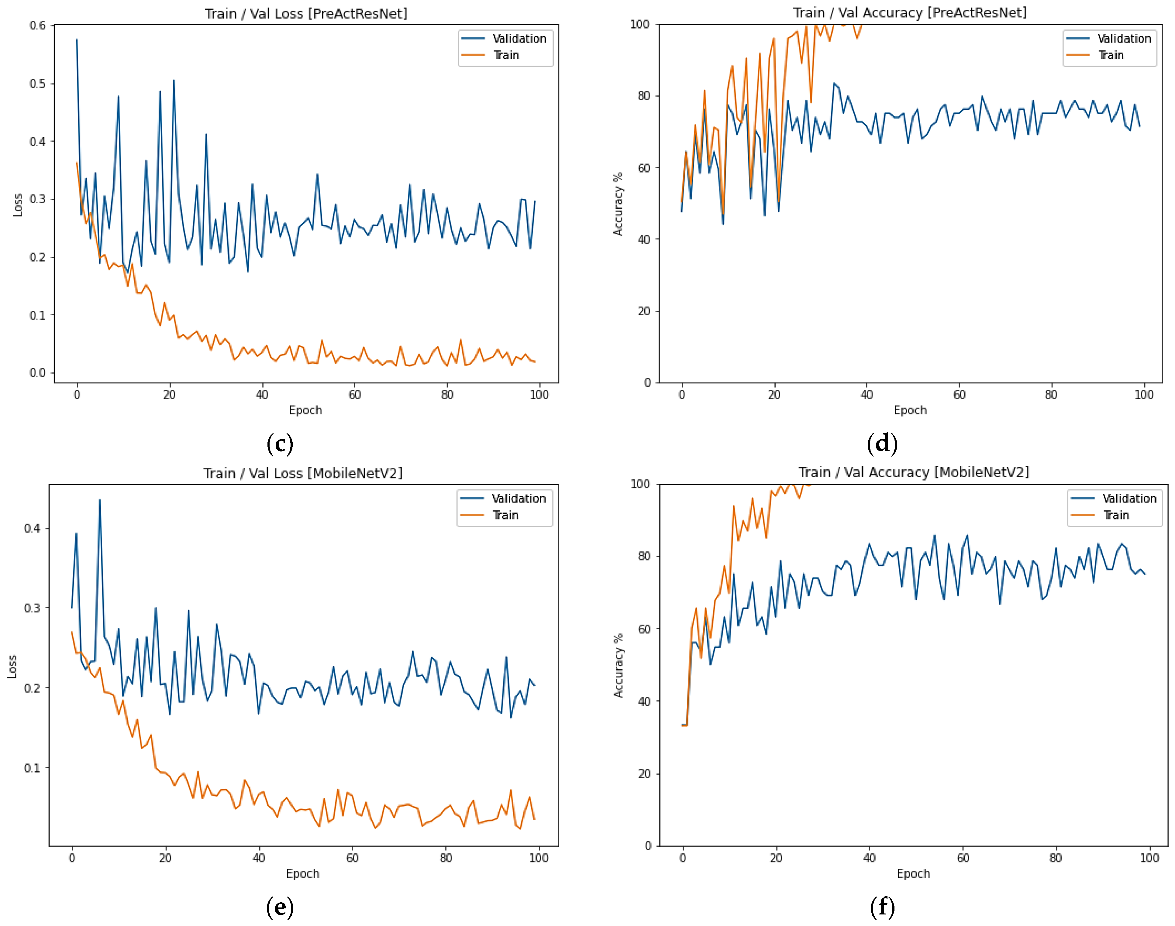
Figure 4 depicts the performance of various classifiers during the training and validation phases. As observed, the training and validation losses in the PreActResNet model exhibit significant oscillations and take longer to train and achieve comparable accuracy as MobilNetV2. While PreActResNet performs as efficiently as MobilNetV2 in terms of accuracy on the training set, it falls short of ResNetV2. On the other hand, although MobilNetV2 has a faster training time, it is unable to attain high accuracy.

3.3. ResNetV2 Classifier Results

Table 3. Confusion matrices on test data for ResNetV2; classes A, B, and C refer to sound, 8 h, and 16 h after bruising, respectively.

		Class A	Class B	Class C
ResNetV2	Class A	6	0	1
	Class B	0	7	0
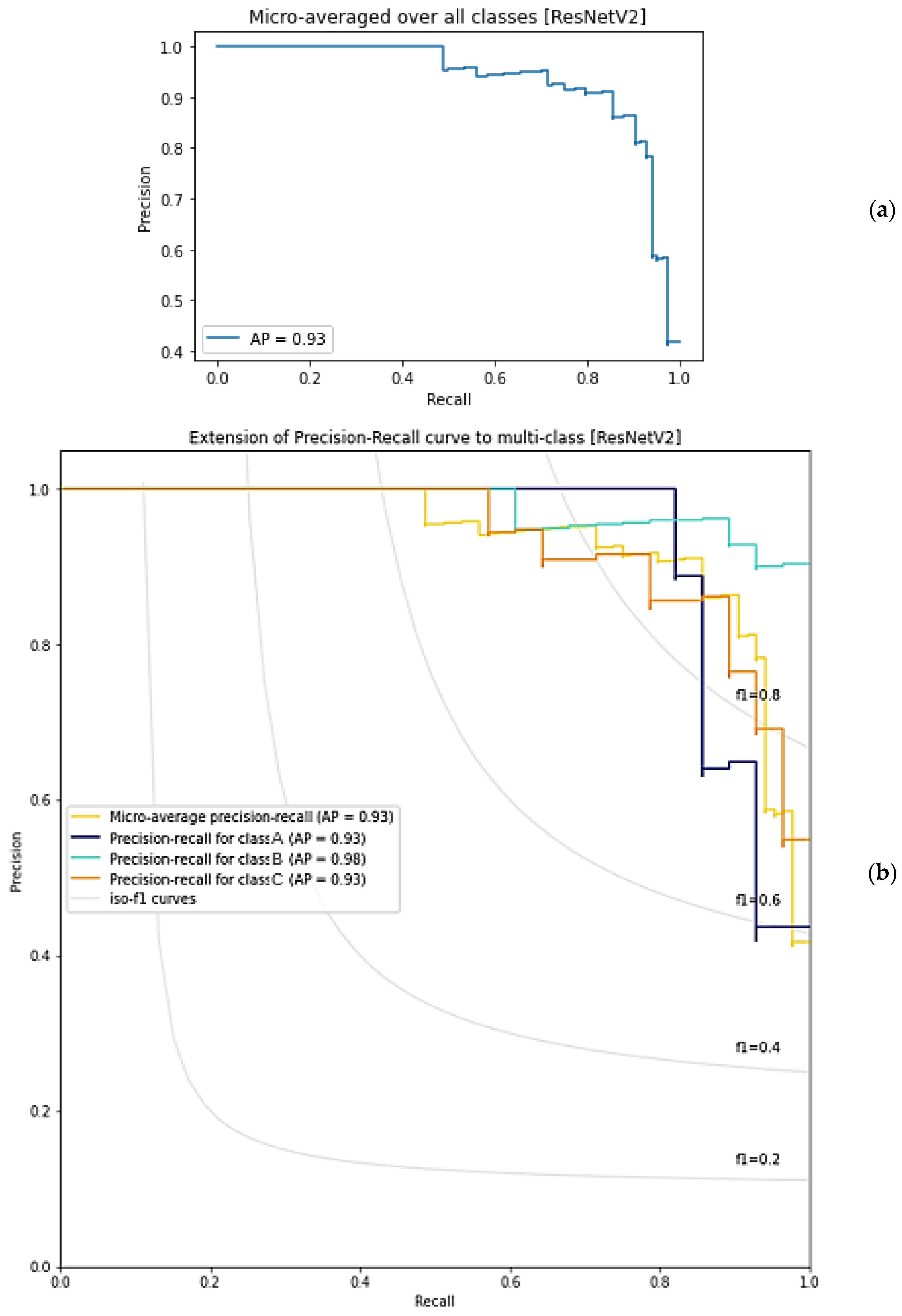
	Class C	0	1	6

presents the confusion matrix for the ResNetV2 classifier. The diagonal values indicate that Class B had the highest accuracy. The model achieved an average precision (AP) of 0.93, with Class B having the best AP of 0.98. This suggests that the model can classify Class B more accurately than other classes. Additionally, Class A and Class C had the same AP of 0.93. The precision–recall curves for the ResNetV2 models are shown in Figure 5.

3.4. PreActResNet Classifier Results

Table 4. Confusion matrices on test data for PreActResNet; Classes A, B, and C refer to sound, 8 h, and 16 h after bruising, respectively.

		Class A	Class B	Class C
PreActResNet	Class A	5	1	1
	Class B	0	7	0
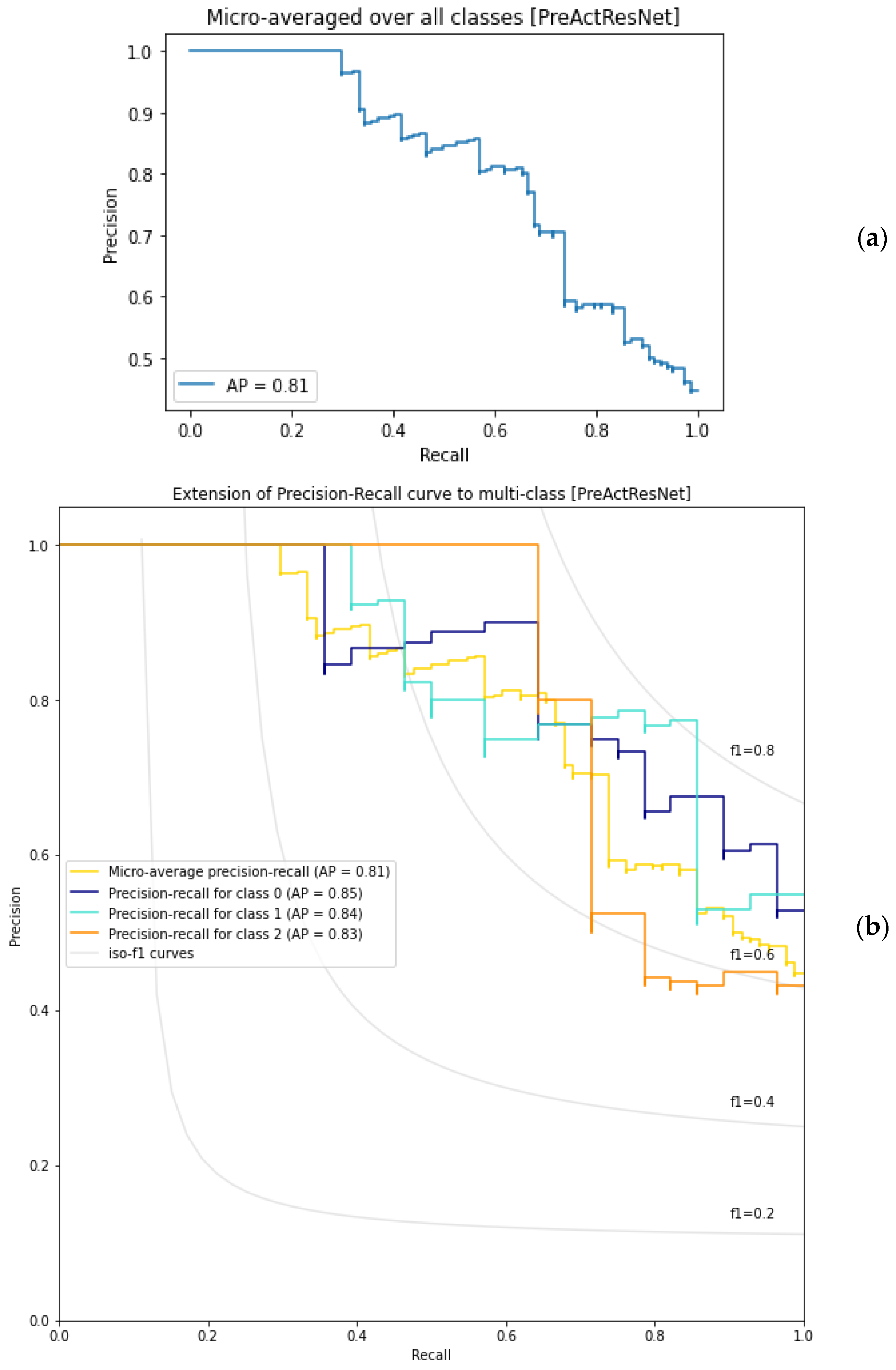
	Class C	1	1	5

displays the confusion matrix for the PreActResNet classifier. The model performs well in predicting Class B samples accurately but struggles in classifying Class A and Class C objects. The AP for this model is 0.81 (Figure 6), which is lower than the ResNetV2 model. Like the ResNetV2 model, the PreActResNet classifier performs the best in distinguishing Class B, but it faces challenges in distinguishing Class C and Class A.

3.5. MobileNetV2 Classifier Results

The confusion matrix for the MobileNetV2 classifier is shown in

Table 5. Confusion matrices on test data for MobileNetv2; Classes A, B, and C refer to sound, 8 h, and 16 h after bruising, respectively.

		Class A	Class B	Class C
MobileNetv2	Class A	6	0	1
	Class B	0	7	0
	Class C	1	1	5

. Like the other two proposed models, the MobileNetV2 classifier has the highest accuracy for Class B. However, its AP is lower than that of PreActResNet and ReseNetV2, at 0.79. The precision–recall curve for MobileNetV2 is shown in Figure 7, which demonstrates that it performs better on Class B than on any other classes.

3.6. Performance Comparison of Classifiers

The performance of the different models in classifying lemon bruising is summarized in

Table 6. Evaluating the proposed models by accuracy, F1-score, and averaged precision (AP).

Model Name	Accuracy %	F1-Score	AP
ResNetV2	92.85	0.9283	0.93
PreActResNet	85.71	0.8540	0.79
MobileNetV2	83.33	0.8315	0.81

, where the accuracy, F1-score, and micro-averaged AP were calculated across all classes. Additionally, the AP was calculated per label. The results show that ResNetV2 offers the highest accuracy. ResNetV2 can be trained faster with fewer parameters that enhance accuracy.

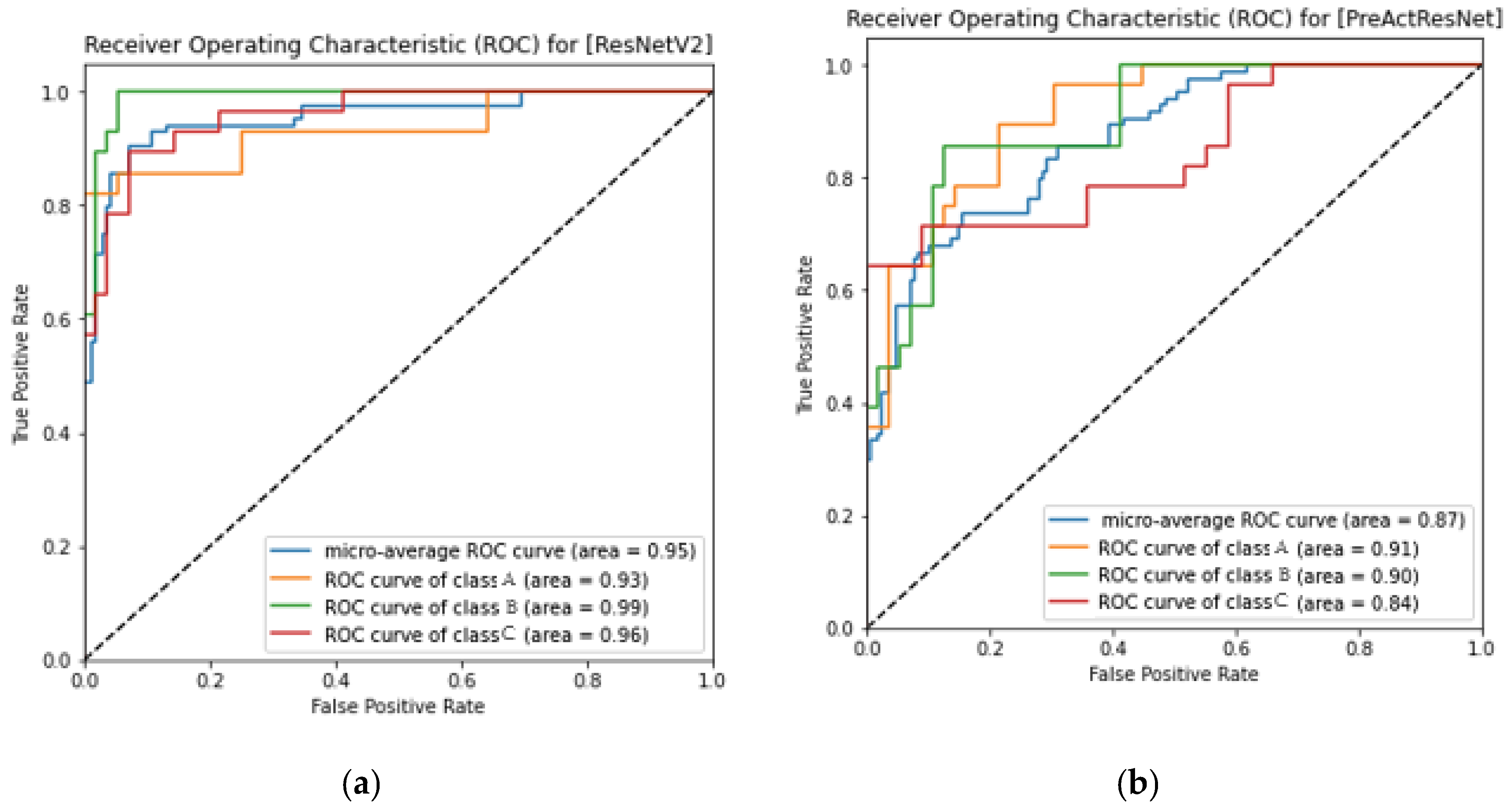
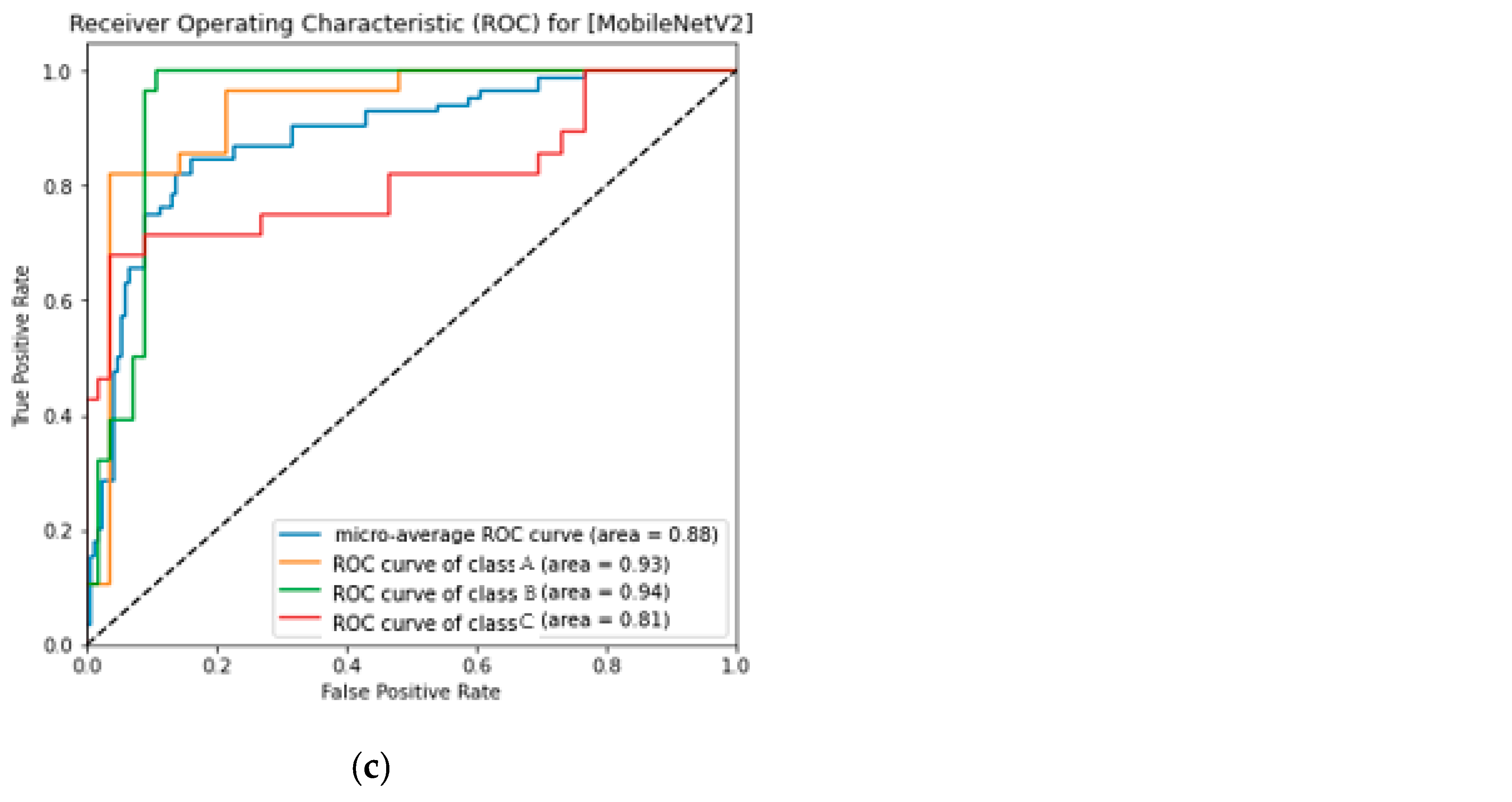
The ROC curves for the three algorithms are depicted in Figure 8. It is evident from the figure that ResNetV2 has the highest ROC value among the three classifiers, and the curves for each class are close to 1 and far from the bisector line, indicating its superior performance in classifying the bruised lemons.

3.7. Interpretation of the ResNetV2 Model

The interpretation of deep-learning models is crucial in the field of image classification. However, the complexity and depth of these models make it challenging to understand their results. To address this issue, various methods exist for interpreting deep-learning models, including visualization. In this study, we utilized Integrated Gradients, a powerful method for interpreting deep-learning models, to identify critical areas or pixels in the input images that contribute to decision making in the developed ResNetV2 model.

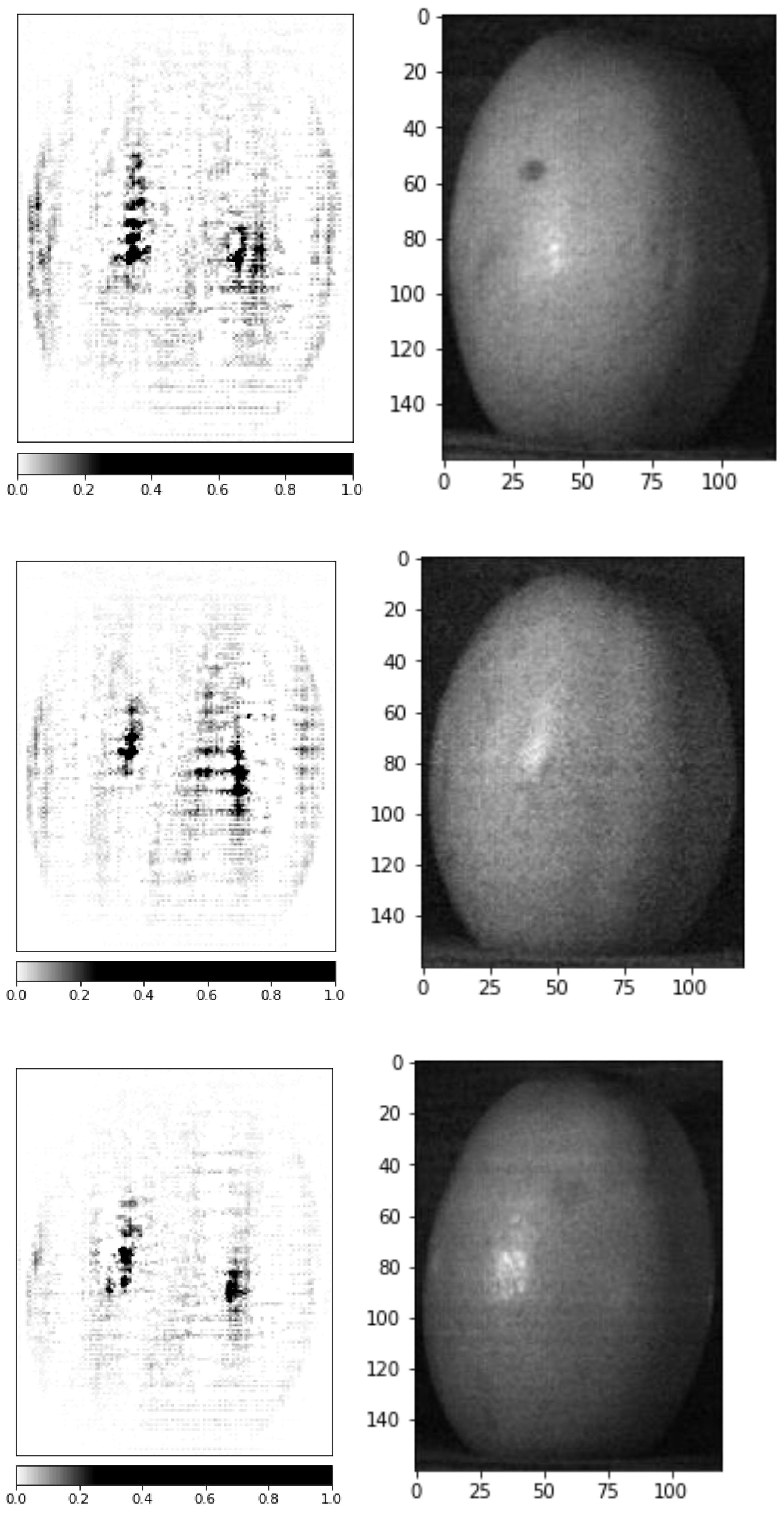
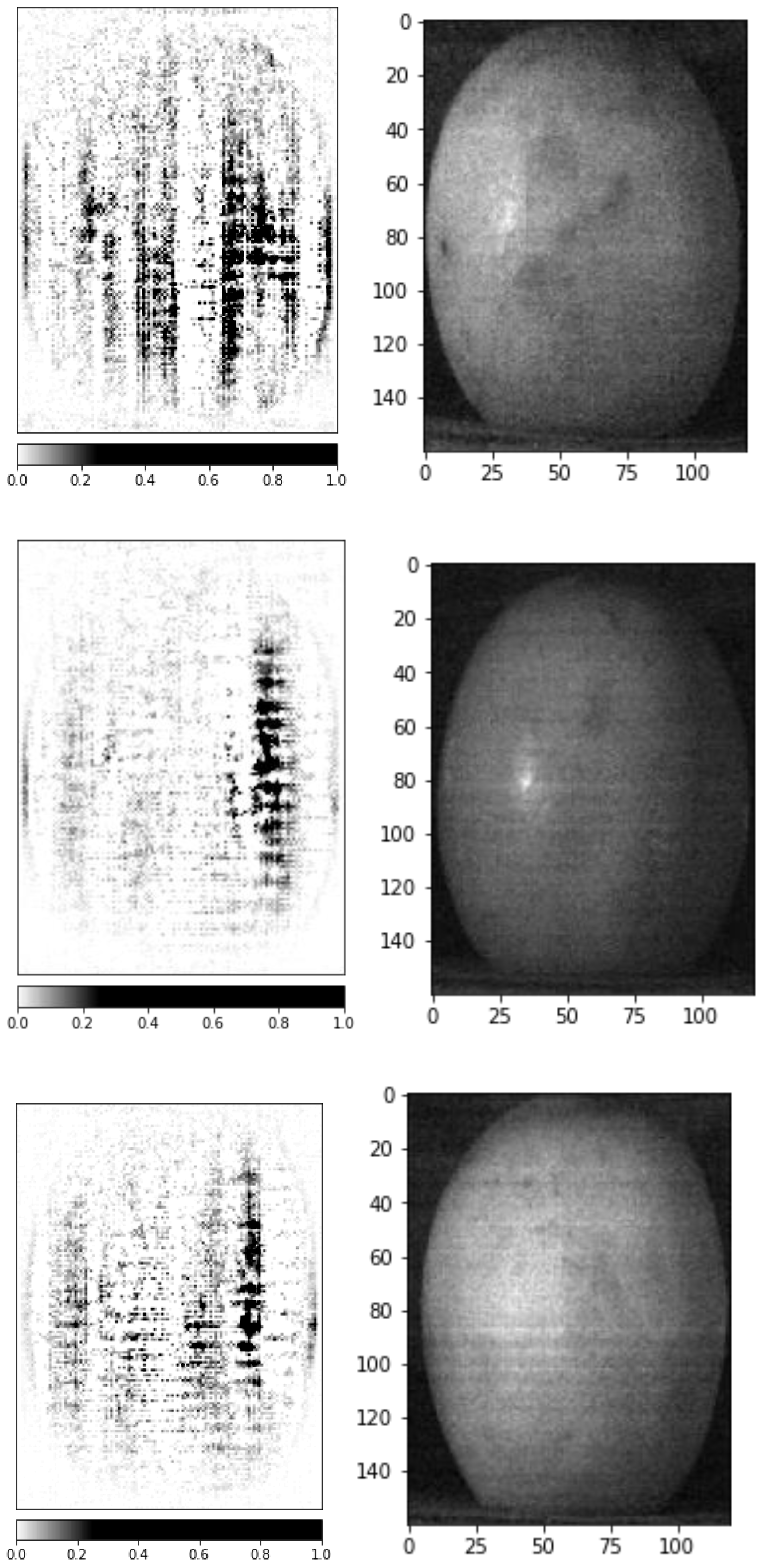
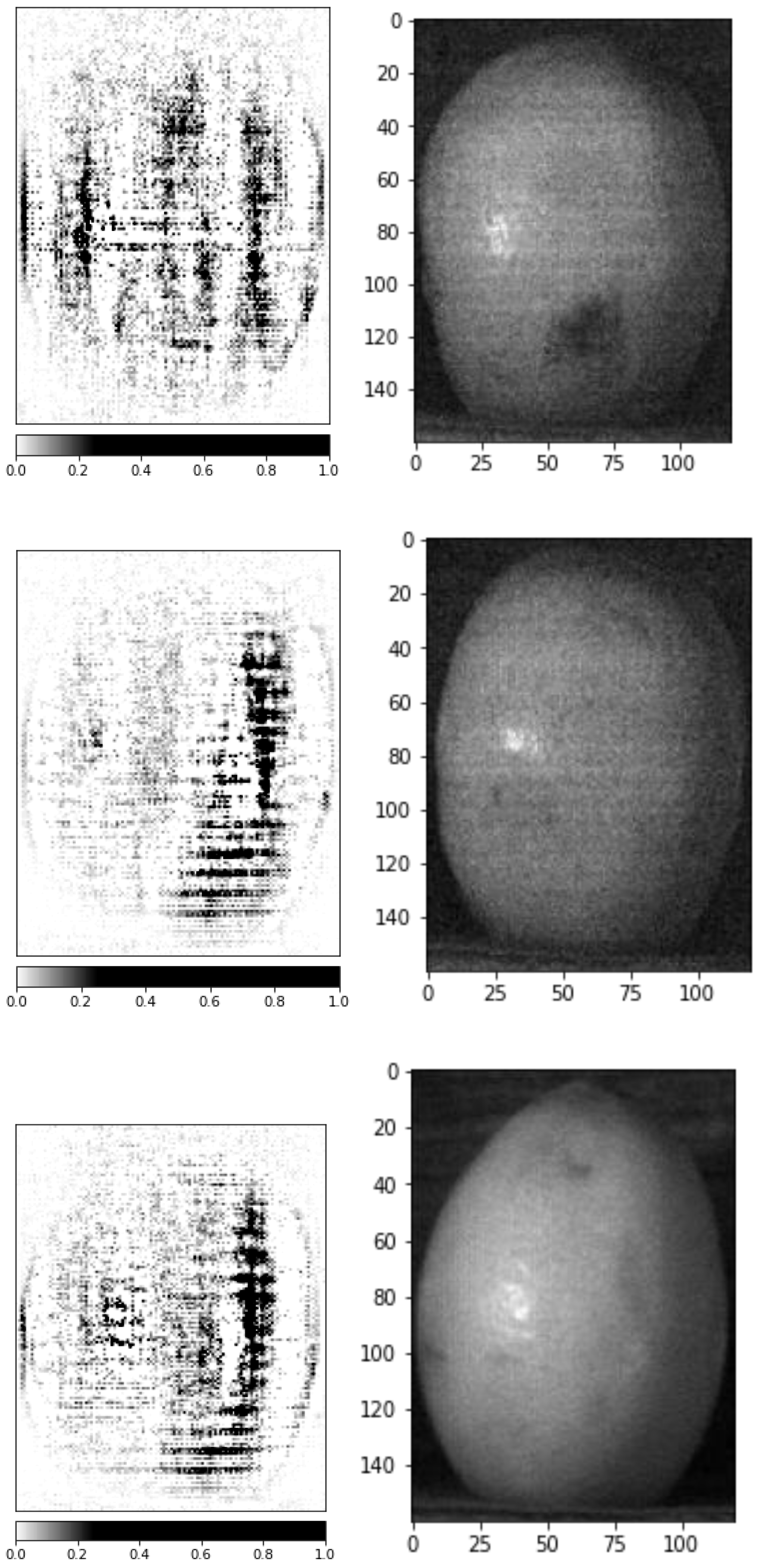
Figure 9, Figure 10 and Figure 11 present the results of Integrated Gradients on three test dataset samples. The left side of each figure shows the Integrated Gradient result, with darker colors indicating higher pixel contributions to the model’s final decision. On the right side of each figure, the original image from the test dataset is displayed. Notably, the ResNetV2 model paid remarkable attention to fruit stains and edges to determine the fruit’s freshness. This approach is reasonable since the stains and edges of a fruit can provide crucial information about its freshness. Using Integrated Gradients for visualization provided valuable insights into the basis of the decision-making process of the ResNetV2 model, thus enhancing the interpretability of its results.

3.8. Comparative Study with Existing Works

Our work introduces the use of advanced CNN-ResNetV2, CNN-MobileNetV2, and CNN-PreActResNet architectures for the identification of bruised lemons, achieving accuracy rates of 92.85%, 83.33%, and 85.71%, respectively. These methods show improvements over other machine-learning models.

To better evaluate the effectiveness of our method, it is beneficial to benchmark our results against related studies. Notably, recent research on bruise detection in lemons using hyperspectral imaging [23] implemented four distinct machine-learning models: ResNet, ShuffleNet, DenseNet, and MobileNet. Their respective classification accuracy amounted to 90.47%, 80.95%, 85.71%, and 73.8%. Remarkably, our study demonstrated superior performance with a 92.85% accuracy, utilizing the ResNetV2 model. The ResNetV2 model, an upgraded version of the commonly used ResNet model, is a profound deep convolutional neural network model often utilized for object detection in images. Contrary to the standard ResNet model, which deploys small square blocks, the ResNetV2 model introduces a “bottleneck block” structure. This structure promotes prioritized training of different network sections and performs network pruning to further enhance its performance. In the same vein, Yang et al. [15] applied polarization imaging and the ResNet-G18 network for the detection of bruised nectarines, achieving a remarkable total classification precision of 96.21%. Yuan et al. [18] employed reflectance, absorbance, and Kubelka-Munk spectral data along with SVM and PLS-DA to discriminate sound and bruised jujube fruit, reporting the highest accuracy of 88.9% using the PLS-DA model. Meanwhile, Munera et al. [20] demonstrated the utility of hyperspectral imaging and PCA in identifying mechanically damaged ‘Rojo Brillante’ persimmon fruits, with a successful detection rate of 90.0%. The promising outcomes of these studies, coupled with our findings, underscore the potential of CNN-based architectures in conjunction with spectral imaging techniques for bruise detection in fruits.

Table 7. Comparison of accuracy between different studies on bruise detection in fruits using various machine-learning models.

Authors	Fruit	Method	Accuracy
Present research	Lemon	CNN-ResNetV2 CNN-MobileNetV2 CNN-PreActResNet	92.85% 83.33% 85.71%
Pourdarbani et al. [23]	Lemon	CNN-DenseNet CNN-ShuffleNet	85.71% 80.95%
		CNN-ResNet	90.47
		CNN-MobileNet	73.80
Yang et al. [15]	Nectarines	CNN-ResNet	97.69%
Yuan et al. [18]	Jujube	SVM and PLS-DA	88.9%
Munera et al. [20]	Persimmons	PCA	90%

provides a comprehensive summary of the studies discussed above, offering a clear comparison of the effectiveness of different methods in bruise detection across various fruits.

3.9. Future Works

In light of the promising findings from this study, several paths for future research present themselves. An important next step would be to investigate the model’s ability to identify different types of natural bruises or to compare artificially induced bruises with natural ones, which could validate the model’s robustness in real-world scenarios. This understanding of the varying characteristics of naturally occurring bruises might further enhance the model’s robustness and generalization capabilities.

Another intriguing avenue for future work involves more granular visualization of the hyperspectral image features related to bruising. Visualizing the feature importance maps or creating a feature graph could provide more insights into how the model interprets and classifies the hyperspectral images. This could also offer a more nuanced understanding of the distinctive spectral characteristics associated with bruising, potentially improving the model’s precision.

Additionally, an ablation study could be incorporated into future research to gain a deeper understanding of the developed models’ architecture and performance. Such a study would shed light on the contribution of each layer or component of the model, providing valuable insights that can be utilized to enhance its overall performance and accuracy.

Moreover, the use of advanced data augmentation techniques, such as Generative Adversarial Networks (GANs), could be considered. While traditional augmentation methods were sufficient for this study, GANs can potentially enrich the dataset, especially in scenarios with limited original data or for larger, more complex datasets, leading to an enhancement in model performance [31].

The automated methods studied here have vast implications for the evolving field of agriculture, particularly in the context of automation and digital transformation. The integration of machine-learning models in crop quality assessment systems could revolutionize the sector by offering a high-speed, non-destructive, and accurate method of fruit quality inspection. Therefore, the advancements presented in this study could substantially contribute to smart agriculture and precision farming.

We also suggest broadening the scope of future research to include other citrus fruits. Extending the techniques employed in this study could enhance the applicability and generalizability of the models, potentially leading to comprehensive quality control systems that span a wide variety of fruit types and conditions.

Lastly, while the present work successfully applied the ResNetV2 model, future work could involve exploring the utilization of other deep-learning models or emerging architectures to improve classification accuracy. Comparative studies between ResNetV2 and these newer models could offer a more comprehensive understanding of their respective strengths and weaknesses, guiding the development of more sophisticated models. Future work could also include the application of these models to other domains of horticulture and the enhancement of the visualization techniques used in this study. Overcoming the challenge of training time in deep-learning models via the use of parallel processing, improved hardware, or more efficient training algorithms could make these models more practical for real-world, time-sensitive applications. While this study focused on detecting bruises on lemons, investigations into the model’s ability to identify other changes, such as ripening stages, pest infestations, or fungal diseases, remain unexplored.

4. Conclusions

This study investigated the effectiveness of three different 3D-CNN architectures, namely ResNetV2, MobileNetV2, and PreActResNet, in detecting bruising in lemons and interpreted the spectral–spatial analysis of the images using Integrated Gradients. The key findings of the study are as follows:

• The ResNetV2 architecture achieved the highest accuracy and was trained faster than the other models;
• The ResNetV2 architecture required more memory despite its short training time;
• The spatial accumulation of dark pixels in hyperspectral images was found to be highly correlated with the presence of fruit bruising, as indicated by the analysis of Integrated Gradients;
• The spectral–spatial interpretation of hyperspectral images by the ResNetV2 architecture showed promising results in detecting bruising in lemons.

The results of this study demonstrate the substantial potential of using 3D-CNN architectures and Integrated Gradients in detecting fruit bruising using hyperspectral imaging. This approach holds promise for a broad range of practical applications, particularly in the agriculture industry, where rapid and accurate detection of crop quality is paramount. For example, the developed models could be implemented in sorting and grading systems in packing houses to automate the quality control process and ensure the delivery of high-quality citrus products. This could help reduce wastage and increase efficiency in supply chains. Moreover, while this study focused on lemons, the employed techniques could potentially be extended to other crops.