Towards a Physiological Modeling of Sweet Cherry Blossom


Abstract
:
1. Introduction
2. Materials and Methods
2.1. Study Area
2.2. Phenological and Meteorological Data
2.3. Physiological Data
2.4. Model Development
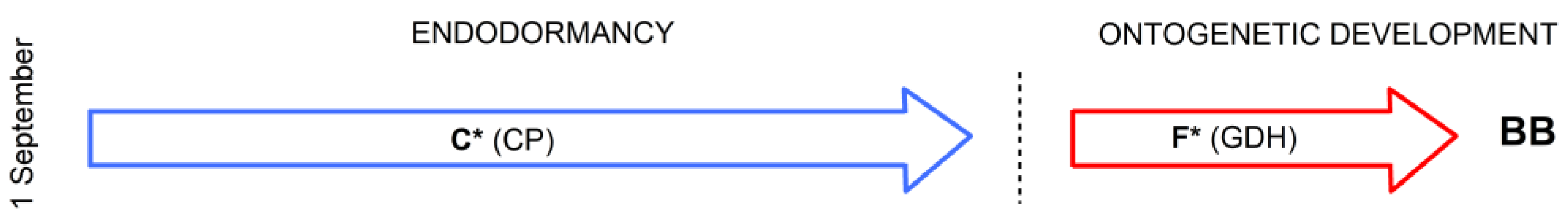
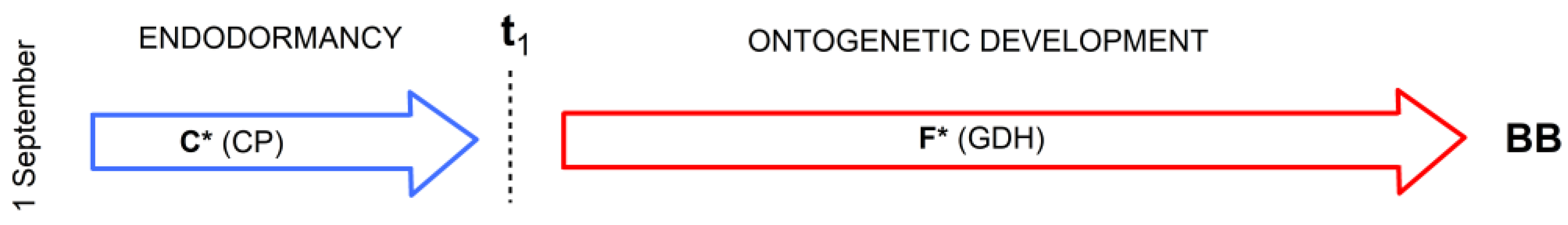
2.4.1. Optimized Classical Two-Phase Model M1
2.4.2. Physiologically Based Two-Phase Model M2
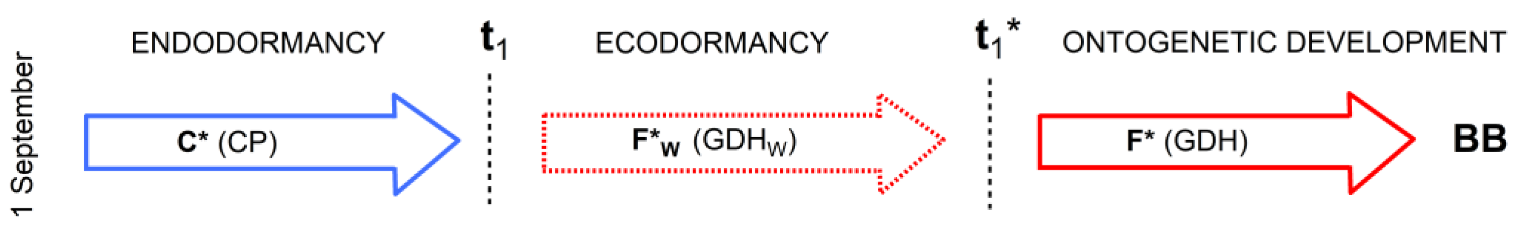
2.4.3. Physiologically Based Three-Phase Model M3
2.5. Model Validation
2.6. Statistical Analysis
3. Results
3.1. Parameter Estimation and Performance of Model M1
3.2. Parameter Estimation and Performance of Model M2
3.3. Parameter Estimation and Performance of Model M3
4. Discussion
4.1. Physiological Parameters Used for Modeling
4.2. Model Comparison
5. Conclusions
Supplementary Materials
Author Contributions
Funding
Data Availability Statement
Acknowledgments
Conflicts of Interest
References
- Lang, G.A.; Early, J.D.; Martin, G.C.; Darnell, R.L. Endodormancy, paradormancy, and ecodormancy—Physiological terminology and classification for dormancy research. Hortscience 1987, 22, 371–377. [Google Scholar] [CrossRef]
- Fadón, E.; Fernandez, E.; Behn, H.; Luedeling, E.A. Conceptual Framework for Winter Dormancy in Deciduous Trees. Agronomy 2020, 10, 241. [Google Scholar] [CrossRef]
- Chmielewski, F.M.; Götz, K.P. Identification and Timing of Dormant and Ontogenetic Phase for Sweet Cherries in Northeast Germany for Modelling Purposes. J. Hortic. 2017, 4, 205. [Google Scholar] [CrossRef]
- Kaufmann, H.; Blanke, M. Substitution of winter chilling by spring forcing for flowering using sweet cherry as a model crop. Sci. Hortic. 2019, 244, 75–81. [Google Scholar] [CrossRef]
- Menzel, A.; Yuan, Y.; Hamann, A.; Ohl, U.; Matiu, M. Chilling and Forcing from Cut Twigs—How to Simplify Phenological Experiments for Citizen Science. Front. Plant Sci. 2020, 11, 561413. [Google Scholar] [CrossRef] [PubMed]
- Fadón, E.; Fernandez, E.; Do, H.T.; Kunz, A.; Krefting, P.; Luedeling, E. Chill and heat accumulation modulates phenology in temperate fruit trees. Acta Hortic. 2021, 1327, 413–420. [Google Scholar] [CrossRef]
- Chmielewski, F.M.; Götz, K.P. ABA and Not Chilling Reduces Heat Requirement to Force Cherry Blossom after Endodormancy Release. Plants 2022, 11, 2044. [Google Scholar] [CrossRef]
- Götz, K.P.; Chmielewski, F.M.; Homann, T.; Huschek, G.; Matzneller, P.; Rawel, H.M. Seasonal changes of physiological parameters in sweet cherry (Prunus avium L.) buds. Sci. Hortic. 2014, 172, 183–190. [Google Scholar] [CrossRef]
- Chuine, I.; Cortazar-Atauri, I.G.; Kramer, K.; Hänninen, H. Plant development models. In Phenology an Integrative Environmental Science, 2nd ed.; Schwartz, M.D., Ed.; Springer Science + Business Media B.V.: Dordrecht, The Netherland, 2013; pp. 275–293. [Google Scholar] [CrossRef]
- Luedeling, E. PhenoFlex—An integrated model to predict spring phenology in temperate fruit trees. Agric. For. Meteorol. 2021, 307, 1084912021. [Google Scholar] [CrossRef]
- Chuine, I.; Bonhomme, M.; Legave, J.M.; Garcia De Cortazar Atauri, I.; Charrier, G.; Lacointe, A.; Améglio, T. Can phenological models predict tree phenology accurately in the future? The unrevealed hurdle of endodormancy break. Glob. Chang. Biol. 2016, 22, 3444–3460. [Google Scholar] [CrossRef]
- Chuine, I.; Régnière, J. Process-Based Models of Phenology for Plants and Animals. Annu. Rev. Ecol. Evol. Syst. 2017, 48, 159–182. [Google Scholar] [CrossRef]
- Cooke, J.E.K.; Eriksson, M.E.; Junttila, O. The dynamic nature of bud dormancy in trees: Environmental control and molecular mechanisms. Plant Cell Environ. 2012, 35, 1707–1728. [Google Scholar] [CrossRef] [PubMed]
- Chmielewski, F.M.; Götz, K.P. Performance of models for the beginning of sweet cherry blossom under current and changed climate conditions. Agric. For. Meteorol. 2016, 218–219, 85–91. [Google Scholar] [CrossRef]
- Campoy, J.A.; Ruiz, D.; Egea, J. Dormancy in temperate fruit trees in a global warming context: A review. Sci. Hortic. 2011, 130, 357–372. [Google Scholar] [CrossRef]
- Richardson, A.D.; Anderson, R.S.; Altaf Arain, M.; Barr, A.G.; Bohrer, G.; Chen, G.; Chen, J.M.; Ciais, P.; Davis, K.J.; Desai, A.R.; et al. Terrestrial biosphere models need better representation of vegetation phenology: Results from the North American Carbon Program Site Synthesis. Glob. Chang. Biol. 2012, 18, 566–584. [Google Scholar] [CrossRef]
- Basler, D. Evaluating phenological models for the prediction of leaf-out dates in six temperate tree species across central Europe. Agric. For. Meteorol. 2016, 217, 10–21. [Google Scholar] [CrossRef]
- Hänninen, H.; Kramer, K.; Tanino, K.; Zhang, R.; Wu, J.; Fu, Y.H. Experiments are necessary in process-based tree phenology modelling. Trends Plant Sci. 2019, 24, 199–209. [Google Scholar] [CrossRef]
- Lundell, R.; Hänninen, H.; Saarinen, T.; Åström, H.; Zhang, R. Beyond rest and quiescence (endodormancy and ecodormancy): A novel model for quantifying plant-environment interaction in bud dormancy release. Plant Cell Environ. 2019, 43, 40–54. [Google Scholar] [CrossRef]
- Egea, J.A.; Egea, J.; Ruiz, D. Reducing the uncertainty on chilling requirements for endodormancy breaking of temperate fruits by data-based parameter estimation of the dynamic model: A test case in apricot. Tree Physiol. 2021, 41, 644–656. [Google Scholar] [CrossRef]
- Singh, R.K.; Svystun, T.; AlDahmash, B.; Jönsson, A.M.; Bhalerao, R.P. Photoperiod- and temperature-mediated control of phenology in trees—A molecular perspective. New Phytol. 2017, 213, 511–524. [Google Scholar] [CrossRef]
- Tylewicz, S.; Petterle, A.; Marttila, S.; Miskolczi, P.; Azeez, A.; Singh, R.K.; Immanen, J.; Mähler, N.; Hvidsten, T.R.; Eklund, D.M.; et al. Photoperiodic control of seasonal growth is mediated by ABA acting on cell–cell communication. Science 2018, 360, 212–215. [Google Scholar] [CrossRef] [PubMed]
- Fadón, E.; Fernandez, E.; Behn, H.; Fadón, E.; Rodrigo, J.; Herrero, M. Is there a specific stage to rest? Morphological changes in flower primordia in relation to endodormancy in sweet cherry (Prunus avium L.). Trees 2018, 32, 1583–1594. [Google Scholar] [CrossRef]
- Beil, I.; Kreyling, J.; Meyer, C.; Lemcke, N.; Malyshev, A.V. Late to bed, late to rise—Warmer autumn temperatures delay spring phenology by delaying dormancy. Glob. Chang. Biol. 2021, 27, 5806–5817. [Google Scholar] [CrossRef]
- Yang, Q.; Gao, Y.; Wu, X.; Bai, T.M.S.; Teng, Y. Bud endodormancy in deciduous fruit trees: Advances and prospects. Hortic. Res. 2021, 8, 139. [Google Scholar] [CrossRef]
- Yamane, H.; Singh, A.K.; Cooke, J.E.K. Plant dormancy research: From environmental control to molecular regulatory networks. Tree Physiol. 2021, 41, 523–528. [Google Scholar] [CrossRef]
- Rinne, P.L.H.; Kaikuranta, P.M.; van der Schoot, C. The shoot apical meristem restores its symplasmic organization during chilling-induced release from dormancy. Plant J. 2001, 26, 249–264. [Google Scholar] [CrossRef]
- Wang, D.; Gao, Z.; Du, P.; Xiao, W.; Tan, Q.; Chen, X.; Li, L.; Gao, D. Expression of ABA metabolism-related genes suggests similarities between seed dormancy and bud dormancy of peach (Prunus persica). Front. Plant Sci. 2016, 6, 1248. [Google Scholar] [CrossRef]
- Pan, W.; Liang, J.; Sui, J.; Li, J.; Liu, C.; Yin, X.; Zhang, Y.; Wang, S.; Zhao, Y.; Zhang, J.; et al. ABA and bud dormancy in perennials: Current knowledge and future perspective. Genes 2021, 12, 1635. [Google Scholar] [CrossRef]
- Rutting, T.; Arend, M.; Morreel, K.; Storme, V.; Rombauts, S.; Fromm, J.; Bhalerao, R.P.; Boerjan, W.; Rhode, A. A molecular timetable for apical bud formation and dormancy in poplar. Plant Cell 2007, 19, 2370–2390. [Google Scholar] [CrossRef]
- Baron, K.D.; Schroeder, D.F.; Stasolla, C. Transcriptional response of abscisic acid (ABA) metabolism and transport to cold and heat stress applied at the reproductive stage of development in Arabidopsis thaliana. Plant Sci. 2012, 188–189, 48–59. [Google Scholar] [CrossRef]
- Castède, S.; Campoy, J.A.; Le Dantec, L.; Quero-García, J.; Barreneche, T.; Wenden, B.; Dirlewanger, E. Mapping of candidate genes involved in bud dormancy and flowering time in sweet cherry (Prunus avium). PLoS ONE 2015, 10, e0143250. [Google Scholar] [CrossRef] [PubMed]
- Liu, J.; Sherif, S.M. Hormonal Orchestration of Bud Dormancy Cycle in Deciduous Woody Perennials. Front Plant Sci. 2019, 10, 1136. [Google Scholar] [CrossRef] [PubMed]
- Vimont, N.; Fouché, M.; Campoy, J.A.; Tong, M.; Arkoun, M.; Yvin, J.C.; Wigge, P.A.; Dirlewanger, E.; Cortijo, S.; Wenden, B. From bud formation to flowering: Transcriptomic state defines the cherry developmental phases of sweet cherry bud Dormancy. BMC Genom. 2019, 20, 974. [Google Scholar] [CrossRef] [PubMed]
- Vimont, N.; Schwarzenberg, A.; Domijan, M.; Donkpegan, A.S.L.; Beauvieux, R.; Le Dantec, L.; Arkoun, M.; Jamois, F.; Yvin, J.-C.; Wigge, P.A.; et al. Fine tuning of hormonal signaling is linked to dormancy status in sweet cherry flower buds. Tree Physiol. 2020, 41, 544–561. [Google Scholar] [CrossRef]
- Wang, D.; Gao, Z.; Li, H.; Jiu, S.; Qu, Y.; Wang, L.; Ma, C.; Xu, W.; Wang, S.; Zhang, C. Dormancy-associated MADS-box (DAM) genes influence chilling requirement of sweet cherries and co-regulate flower development with SOC1 gene. Int. J. Mol. Sci. 2020, 21, 921. [Google Scholar] [CrossRef]
- Chmielewski, F.M.; Götz, K.P. Metabolites in cherry buds to detect winter dormancy. Metabolites 2022, 12, 247. [Google Scholar] [CrossRef]
- Chmielewski, F.M.; Baldermann, S.; Götz, K.P.; Homann, T.; Gödeke, K.; Schumacher, F.; Huschek, G.; Rawel, H.M. Abscisic Acid Related Metabolites in Sweet Cherry Buds (Prunus avium L.). J. Hortic. 2018, 5, 221. [Google Scholar] [CrossRef]
- Götz, K.P.; Chmielewski, F.M. Metabolites That Confirm Induction and Release of Dormancy Phases in Sweet Cherry Buds. Metabolites 2023, 13, 231. [Google Scholar] [CrossRef]
- Hänninen, H. Boreal and Temperate Trees in a Changing Climate: Modelling the Ecophysiology of Seasonality, Biometeorology 3; Springer Science + Business Media: Dordrecht, The Netherland, 2016; p. 342. [Google Scholar]
- Meier, U. Growth Stages of Mono-and Dicotyledonous Plants. BBCH Monograph; Open Agrar Repositorium: Quedlinburg, Germany, 2018; p. 204. [Google Scholar] [CrossRef]
- Fishman, S.; Erez, A.; Couvillon, G.A. The temperature dependence of dormancy breaking in plants: Mathematical analysis of a two-step model involving a cooperative transition. J. Theor. Biol. 1987, 124, 473–483. [Google Scholar] [CrossRef]
- Fishman, S.; Erez, A.; Couvillon, G.A. The temperature dependence of dormancy breaking in plants: Computer simulation of processes studied under controlled temperatures. J. Theor. Biol. 1987, 126, 309–321. [Google Scholar] [CrossRef]
- Anderson, J.L.; Richardson, E.A.; Kesner, C.D. Validation of chill unit and flower bud phenology models for ‘Montmorency’ sour cherry. Acta Hortic. 1986, 184, 71–75. [Google Scholar] [CrossRef]
- Tsallis, C.; Stariolo, D.A. Generalized simulated annealing. Phys. A Stat. Mech. Its Appl. 1996, 233, 395–406. [Google Scholar] [CrossRef]
- Press, W.H.; Teukolsky, S.A.; Vetterling, W.T.; Flannery, B.P. Numerical Recipes in Fortran 77. In The Art of Scientific Computing, 2nd ed.; Cambrigde Unversity Press: Cambrigde, UK, 1997; p. 994. [Google Scholar]
- Burla, B.; Pfrunder, S.; Nagy, R.; Francisco, R.M.; Lee, Y.; Martinoia, E. Vacuolar transport of abscisic acid glucosyl ester is mediated by ATP-binding cassette and proton-antiport mechanisms in Arabidopsis. Plant Physiol. 2013, 163, 1446. [Google Scholar] [CrossRef]
- Brown, D.S.; Kotob, F.A. Growth of flower buds of apricot, peach, and pear during the rest period. Proc. Am. Soc. Hortic. Sci. 1957, 69, 158–164. [Google Scholar]
- Cannell, M.G.R.; Smith, R.I. Thermal time, chill days and prediction of budburst in Picea sitchensis. J. Appl. Ecol. 1983, 20, 951–963. [Google Scholar] [CrossRef]
- Hsiang, T.-F.; Lin, Y.-J.; Yamane, H.; Tao, R. Characterization of Japanese Apricot (Prunus mume) Floral Bud Development Using a Modified BBCH Scale and Analysis of the Relationship between BBCH Stages and Floral Primordium Development and the Dormancy Phase Transition. Horticulturae 2021, 7, 142. [Google Scholar] [CrossRef]
- Fadón, E.; Herrera, S.; Herrero, M.; Rodrigo, J. Male meiosis in sweet cherry is constrained by the chilling and forcing phases of dormancy. Tree Physiol. 2021, 41, 619–630. [Google Scholar] [CrossRef]
- Zeng, X.; Du, Y.; Vitasse, Y. Untangling winter chilling and spring forcing effects on spring phenology of subtropical tree seedlings. Agric. For. Meteorol. 2023, 335, 109456. [Google Scholar] [CrossRef]
- Ashcroft, G.L.; Richardson, E.A.; Seeley, S.D. A statistical method of determining Chill Unit and Growing. Degree Hour requirements for deciduous fruit trees. HortScience 1977, 12, 347–348. [Google Scholar] [CrossRef]
- Kramer, K. A modelling analysis of the effects of climatic warming on the probability of spring frost damage to tree species in the Netherlands and Germany. Plant Cell Environ. 1994, 17, 367–377. [Google Scholar] [CrossRef]
- Chuine, I.; Cour, P.; Rousseau, D.D. Fitting models predicting dates of flowering of temperate-zone trees using simulated annealing. Plant Cell Environ. 1998, 21, 455–466. [Google Scholar] [CrossRef]
- Linkosalo, T.; Häkkinen, R.; Hänninen, H. Models of the spring phenology of boreal and temperate trees: Is there something missing? Tree Physiol. 2006, 26, 1165–1172. [Google Scholar] [CrossRef] [PubMed]
- Fu, Y.H.; Campioli, M.; Van Oijen, M.; Deckmyn, G.; Janssens, I.A. Bayesian comparison of six different temperature-based budburst models for four temperate tree species. Ecol. Model. 2012, 230, 92–100. [Google Scholar] [CrossRef]
- Wang, X.; Xu, H.; Ma, Q.; Luo, Y.; He, D.; Smith, N.G.; Rossi, S.; Chen, L. Chilling and forcing proceed in parallel to regulate spring leaf unfolding in temperate trees. Glob. Ecol. Biogeogr. 2023, 32, 1914–1927. [Google Scholar] [CrossRef]
- Zhang, R.; Lin, J.; Wang, F.; Delpierre, N.; Kramer, K.; Hänninen, H.; Wu, J. Spring phenology in subtropical trees: Developing process-based models on an experimental basis. Agric. For. Meteorol. 2022, 31, 108802. [Google Scholar] [CrossRef]
- Luedeling, E.; Gassner, A. Partial Least Squares regression for analysing walnut phenology in California. Agric. For. Meteorol. 2012, 158, 43–52. [Google Scholar] [CrossRef]
- Luedeling, E.; Kunz, A.; Blanke, M.M. Identification of chilling and heat requirements of cherry trees—A statistical approach. Int. J. Biometeorol. 2013, 57, 679–689. [Google Scholar] [CrossRef]
- Drogoudi, P.; Cantín, C.M.; Brandi, F.; Butcaru, A.; Cos-Terrer, J.; Cutuli, M.; Foschi, S.; Galindo, A.; García-Brunton, J.; Luedeling, E.; et al. Impact of Chill and Heat Exposures under Diverse Climatic Conditions on Peach and Nectarine Flowering Phenology. Plants 2023, 12, 584. [Google Scholar] [CrossRef]
- Fadón, E.; Espiau, M.T.; Errea, P.; Alonso Segura, J.M.; Rodrigo, J. Agroclimatic Requirements of Traditional European Pear (Pyrus communis L.) Cultivars from Australia, Europe, and North America. Agronomy 2023, 13, 518. [Google Scholar] [CrossRef]
- Sapkota, S.; Liu, J.; Islam, M.T.; Rivindran, P.; Kumar, P.P.; Sherif, S.M. Contrasting bloom dates in two apple cultivars linked to differential levels of phytohormones and heat requirements. Sci. Hortic. 2021, 288, 110413. [Google Scholar] [CrossRef]

| Season | 2011/12 | 2012/13 | 2013/14 | 2014/15 | 2015/16 | 2016/17 | 2017/18 | 2018/19 | 2019/20 | x | s |
|---|---|---|---|---|---|---|---|---|---|---|---|
| t1 in DOY | 335 | 332 | 323 | 343 | 328 | 341 | 340 | 333 | 339 | 334.9 | 6.6 |
| C* in CP | 42 | 43 | 40 | 40 | 41 | 46 | 49 | 40 | 41 | 42.4 | 3.1 |
| t1* in DOY | 45 | 85 | 35 | 41 | 61 | 45 | 59 | 45 | 51 | 51.9 | 14.9 |
| BB in DOY | 105 | 116 | 95 | 111 | 111 | 97 | 108 | 99 | 105 | 105.2 | 8.5 |
| Season | a | b | R2 | p |
|---|---|---|---|---|
| 2011/12 | 2.9410 | −0.0062 | 0.91 | <0.001 |
| 2012/13 | 2.4044 | −0.0047 | 0.89 | <0.001 |
| 2013/14 | 2.8191 | −0.0053 | 0.80 | <0.001 |
| 2014/15 | 2.9890 | −0.0058 | 0.97 | <0.001 |
| 2015/16 | 2.8390 | −0.0057 | 0.95 | <0.001 |
| 2016/17 | 3.6243 | −0.0076 | 0.95 | <0.001 |
| 2017/18 | 2.2479 | −0.0040 | 0.84 | <0.001 |
| 2018/19 | 3.2097 | −0.0065 | 0.96 | <0.001 |
| 2019/20 | 1.9284 | −0.0029 | 0.56 | <0.001 |
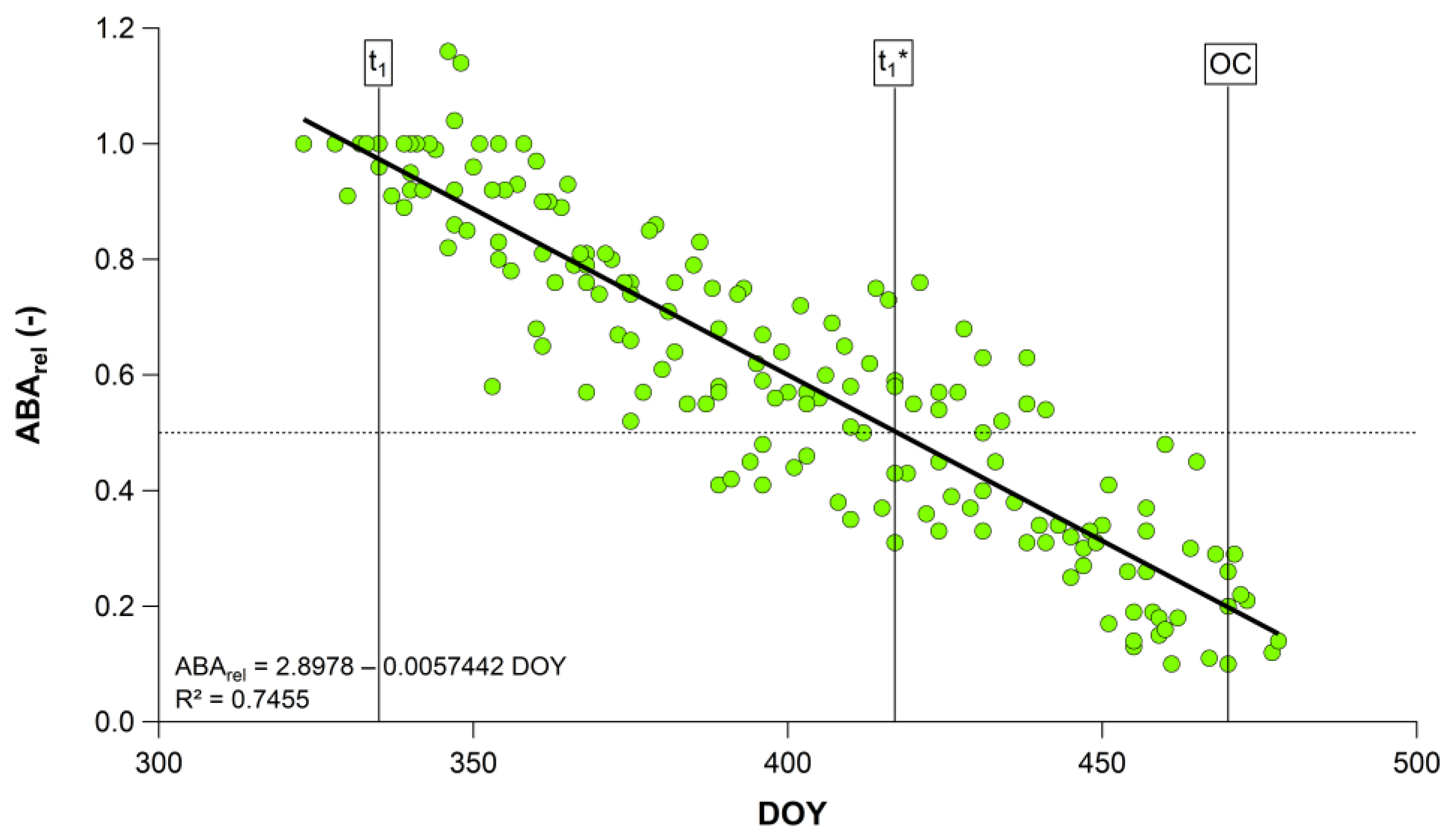
| 2011/12–2019/20 | 2.8978 | −0.0057 | 0.75 | <0.001 |
| Season | t1(92 CP) in DOY | F(t1 − BB) in GDH | BB in DOY | BBcal in DOY | Diff in d |
|---|---|---|---|---|---|
| (a) Calculation of model parameters | |||||
| 2011/12 | 53 | 3012 | 105 | 111 | 6 |
| 2012/13 | 62 | 3444 | 116 | 116 | 0 |
| 2013/14 | 38 | 3645 | 95 | 94 | −1 |
| 2014/15 | 56 | 3217 | 111 | 113 | 2 |
| 2015/16 | 38 | 3278 | 111 | 114 | 3 |
| 2016/17 | 53 | 3226 | 97 | 99 | 2 |
| 2017/18 | 40 | 4003 | 108 | 106 | −2 |
| 2018/19 | 42 | 3879 | 99 | 97 | −2 |
| 2019/20 | 40 | 4165 | 105 | 101 | −4 |
| x | 47 | 3541 | 105.2 | 105.7 | |
| s | 9.1 | 401.6 | 7.1 | 8.2 | MAE = 2.44 d |
| cv | 19.4 | 11.3 | 6.7 | 7.7 | RMSE = 2.62 d |
| (b) Model Validation with C* = 96 CP, F* = 3541 GDH | |||||
| 2020/21 | 56 | 3546 | 110 | 117 | 7 |
| 2021/22 | 41 | 3541 | 109 | 107 | −2 |
| 2022/23 | 47 | 3541 | 112 | 111 | −1 |
| MAE = 3.33 d | |||||
| RMSE = 4.24 d | |||||
| Season | F(t1 − t1*) in GDH | F(t1* − BB) in GDH | F(t1 − BB) in GDH | BB in DOY | BBcal in DOY | Diff in d |
|---|---|---|---|---|---|---|
| (a) Calculation of model parameters | ||||||
| 2011/12 | 642 | 3029 | 3671 | 105 | 112 | 7 |
| 2012/13 | 645 | 3315 | 3960 | 116 | 120 | 4 |
| 2013/14 | 802 | 3664 | 4466 | 95 | 95 | 0 |
| 2014/15 | 744 | 3290 | 4034 | 111 | 114 | 3 |
| 2015/16 | 2460 | 3050 | 5510 | 111 | 100 | −11 |
| 2016/17 | 312 | 3378 | 3690 | 97 | 104 | 7 |
| 2017/18 | 763 | 3998 | 4761 | 108 | 107 | −1 |
| 2018/19 | 711 | 3848 | 4559 | 99 | 98 | −1 |
| 2019/20 | 1900 | 3685 | 5585 | 105 | 98 | −7 |
| x | 998 | 3473 | 4471 | 105.2 | 105.3 | |
| s | 699.4 | 343.0 | 717.2 | 7.1 | 8.5 | MAE = 4.56 d |
| cv | 70.1 | 9.9 | 16.0 | 6.7 | 8.1 | RMSE = 5.23 d |
| (b) Model Validation with F*(t1 − BB) = 4471 GDH | ||||||
| 2020/21 | 756 | 3714 | 4479 | 110 | 111 | 1 |
| 2021/22 | 1488 | 3459 | 4947 | 109 | 104 | −5 |
| 2022/23 | 1845 | 3191 | 5036 | 112 | 104 | −8 |
| MAE = 4.67 d | ||||||
| RMSE = 5.48 d | ||||||
| Season | FW(t1 − t1*) in GDHW | F(t1* − BB) in GDH | F(t1 − BB) in GDH* | BB in DOY | BBcal in DOY | Diff in d |
|---|---|---|---|---|---|---|
| (a) Calculation of model parameters | ||||||
| 2011/12 | 183 | 3029 | 3212 | 105 | 110 | 5 |
| 2012/13 | 254 | 3315 | 3569 | 116 | 116 | 0 |
| 2013/14 | 71 | 3664 | 3735 | 95 | 94 | −1 |
| 2014/15 | 90 | 3290 | 3380 | 111 | 113 | 2 |
| 2015/16 | 606 | 3050 | 3656 | 111 | 111 | 0 |
| 2016/17 | 17 | 3378 | 3395 | 97 | 99 | 2 |
| 2017/18 | 188 | 3998 | 4186 | 108 | 105 | −3 |
| 2018/19 | 93 | 3850 | 3943 | 99 | 97 | −2 |
| 2019/20 | 347 | 3685 | 4032 | 105 | 102 | −3 |
| x | 205 | 3473 | 3679 | 105.2 | 105.2 | |
| s | 181.4 | 343.3 | 327.0 | 7.1 | 7.7 | MAE = 2.00 d |
| cv | 88.3 | 9.9 | 8.9 | 6.7 | 7.3 | RMSE = 2.29 d |
| (b) Model Validation with F*(t1 − BB) = 3679 GDH* | ||||||
| 2020/21 | 192 | 3492 | 3684 | 110 | 110 | 0 |
| 2021/22 | 422 | 3459 | 3881 | 107 | 106 | −1 |
| 2022/23 | 496 | 3191 | 3687 | 112 | 111 | −1 |
| MAE = 0.76 d | ||||||
| RMSE = 0.82 d | ||||||
Disclaimer/Publisher’s Note: The statements, opinions and data contained in all publications are solely those of the individual author(s) and contributor(s) and not of MDPI and/or the editor(s). MDPI and/or the editor(s) disclaim responsibility for any injury to people or property resulting from any ideas, methods, instructions or products referred to in the content. |
© 2023 by the authors. Licensee MDPI, Basel, Switzerland. This article is an open access article distributed under the terms and conditions of the Creative Commons Attribution (CC BY) license (https://creativecommons.org/licenses/by/4.0/).
Share and Cite
Chmielewski, F.-M.; Götz, K.-P. Towards a Physiological Modeling of Sweet Cherry Blossom. Horticulturae 2023, 9, 1207. https://doi.org/10.3390/horticulturae9111207
Chmielewski F-M, Götz K-P. Towards a Physiological Modeling of Sweet Cherry Blossom. Horticulturae. 2023; 9(11):1207. https://doi.org/10.3390/horticulturae9111207
Chicago/Turabian StyleChmielewski, Frank-M., and Klaus-Peter Götz. 2023. "Towards a Physiological Modeling of Sweet Cherry Blossom" Horticulturae 9, no. 11: 1207. https://doi.org/10.3390/horticulturae9111207
APA StyleChmielewski, F.-M., & Götz, K.-P. (2023). Towards a Physiological Modeling of Sweet Cherry Blossom. Horticulturae, 9(11), 1207. https://doi.org/10.3390/horticulturae9111207