Willingness-to-Pay for Produce: A Meta-Regression Analysis Comparing the Stated Preferences of Producers and Consumers

Abstract

Willingness-to-pay (WTP) estimates help agribusinesses estimate whether a new product is likely to be profitable. For produce, new products, such as new fruit varieties, need to be adopted by producers before they can be sold to consumers. The study of ex ante fruit and vegetable producer preferences is relatively new. This study uses meta-regression analysis to compare the estimated WTP premium between U.S. producers and consumers to determine whether they differ. After controlling for differences in study methods, product attributes, and potential publication bias, the producer WTP was between 14.16 and 27.73 percentage points higher. Subject to several caveats and limitations, this suggests that consumer WTP can be a sufficient metric for the profitability of new produce products.

1. Introduction

The market for produce is increasingly differentiated, with consumers able to choose between a host of experience attributes, such as color, size, flavor, and credence attributes, such as organic, GM, or locally grown. Each of these options may factor into a consumer’s decision to purchase and affect the amount they are willing to spend on the product. When an agribusiness considers bringing a new product to market, it is essentially proposing to introduce a new bundle of experience and credence attributes to consumers [1,2].

Developing new varieties or introducing novel crops to market is a slow and expensive process. For example, the ‘Covington’ sweetpotato was first identified in 1997 and was released to the public eight years later [3]. Similarly, the ‘WA 38’ apple was first crossed in 1997, released to growers in 2014, and presented to the public as ‘Cosmic Crisp’ in 2019 with a marketing campaign in excess of 10 million dollars [4,5,6].

Before embarking on a new venture, the developer (and its financial backers) would like to know whether there is a market for the new product, or, if there are multiple potential products, which would be most successful. In other words, are they likely to see a positive net return from the time and effort involved in development? Their net return will depend on the costs of development and the revenues from sales. Thus, a reliable forecast of net returns requires a reliable forecast of consumer demand for the new product.

Economists have developed tools for estimating demand for hypothetical and novel products before they come to market. These tools, including experimental auctions, contingent valuation, and conjoint analysis, are able to estimate subjects’ willingness-to-pay (WTP) for a hypothetical or novel product or to estimate the WTP for particular attributes of the product [7]. These WTP estimates can be used to construct demand curves for use in estimating the net returns from the new production. The majority of studies looking at demand for novel or hypothetical produce are looking at the final consumers’ demand, e.g., shoppers in the supermarket. However, for new produce to make it to the consumer, it first must be adopted and grown by producers, whose adoption criteria may differ from those of consumers.

Producers’ WTP can be affected by factors, such as the marketable yield levels, production costs, and ease of harvest, which may or may not correlate with the traits consumers find desirable [8]. Yue and co-authors [8] provided the example of tart cherries, where growers place a high value on firmness, which prevents damage during harvest, while consumers are indifferent to firmness since tart cherries are usually sold as processed, dried, or as juice.

The main goal of this paper is to explore any divergence between producer and consumer WTP for produce. Produce generally refers to fruits and vegetables; in this study, it also includes processed versions of these crops. If, in general, producer WTP is similar to consumer WTP, or higher, then an agribusiness considering introducing a new product on the basis of a sufficiently high consumer WTP can be confident that producers are likely to adopt it, too. On the other hand, if producers have a lower WTP, then innovators run the risk that their product will fail in the market due to insufficient adoption by producers even if the consumer market appears to be present.

No existing reviews or meta-regression analyses of preferences for produce focus on the differences between producers and consumers. Some existing reviews have focused on consumer preferences for food traits, such as sustainability [9,10], health benefits [11,12], or local production [13]. Each of these reviews found that consumers were willing to pay higher premiums for these credence attributes.

Others considered the characteristics of producers, such as their willingness to adopt new technologies [14] or preferences over contract types [15]. In these cases, no special emphasis was placed on produce, and the included papers that did study produce were captured as part of a wider search. In contrast, reviews that did focus on produce looked only at consumer preferences [2,16].

After controlling for potential publication bias, year fixed effects, differences in methods, and differences in attributes studied, this study found that producer WTP percentage premium (WTPP) was on average 21.17 percentage points higher than the consumer WTPP for produce, with a 95 percent confidence interval of 14.61 to 27.73 percentage points, providing initial evidence that consumer WTP studies may be sufficient for estimating potential producer adoption.

1.1. Willingness-to-Pay

Willingness-to-pay (WTP) is the maximum income a consumer would be willing to give up in exchange for a change in the price or quality of the good, while keeping their utility constant (Utility is a measure of the total satisfaction that a consumer receives from the goods and services they consume). For example, in the case of a quality improvement, the increase in quality would increase their utility, and thus their income must be reduced by an amount to exactly offset the quality-induced increase in utility. This amount is the consumer’s WTP.

The WTP concept can be extended to producers in a straightforward manner. Instead of utility, producers’ WTP is calculated by keeping their profit constant. Increasing the quality of an input could increase their profit by increasing yields. The producer’s WTP for the change in the input is the difference in profit before and after the change [7].

This definition assumes a discrete change in the quality or price of the good. Alternatively, the marginal WTP (MWTP) may be calculated and reported, which is the change in WTP with respect to a marginal change in the price or quality. It represents, depending on the context, the first derivative of the value, expenditure, indirect utility, or profit function [17].

In an agribusiness setting, WTP measures can be used to estimate the demand for novel or hypothetical products, guiding firms’ pricing and marketing decisions before the product is launched [7]. With a measure of the distribution of WTP in a potential market in hand, the firm can construct an estimate of the demand curve for the product and, hence, identify its profit-maximizing pricing strategy or offering of product attributes and qualities.

Researchers typically present estimated WTP in four main ways as illustrated with examples from this analysis:

• As a dollar value, e.g., Yue et al. [8] found that U.S. apple growers would be willing to pay $0.16/lb to improve apple size from less than to larger than 2.9 inches.
• As a percentage premium, e.g., Onozaka et al. [18] found that consumers in Northern California were willing to pay a 15 percent price premium for bananas labeled “pesticide free’’ compared to bananas without the label.
• As a probability of adoption for a given price, e.g., Blend and van Ravenswaay [19] found that 72.6 percent of U.S. consumers were willing to purchase eco-labeled apples with zero price premium (compared to unlabeled apples), while 52.4 percent would purchase at a $0.20 price premium, falling to 42.3 percent with a $0.40 price premium.
• As an own- or cross-price elasticity, e.g., Bernard and Bernard [20] found that consumers in four Atlantic coast states would decrease their purchases of conventional potatoes by 3.15 percent in response to a one percent increase in the price of conventional potatoes, while purchases of organic potatoes would rise by 1.20 percent in response to this price increase.

From these estimates, demand curves can be derived (e.g., [21]), which Lusk and Hudson [7] argue are objects of interest for agribusinesses, since they can be used to determine the potential revenues from the new product.

1.2. Methods Used to Measure WTP

To measure WTP, researchers typically turn to choice-modeling methods, which provide opportunities to observe how consumers choose products to purchase and how they make trade offs between similar goods. Choice modeling methods come in two varieties: revealed preference methods and stated preference methods. Revealed preference methods use observed choices, while stated preference methods rely on asking how the respondent would choose, if they were faced with the choice [22].

Experimental auctions (EA) are a common revealed preference technique where subjects bid real money on a good, with the underlying assumption that participants will not bid more than their valuation of the good [23]. While EAs are exposed to less risk of hypothetical bias, since any transactions are binding, they can be time intensive and costly compared to survey instruments [7]. Additionally, since they require real transactions, the goods on which consumers are bidding must already exist, which does not allow for preferences for hypothetical goods to be captured while products are in development. Many market researchers, therefore, turn to choice experiments.

Choice experiments are part of a subset of choice modeling approaches in which subjects are asked to evaluate a set of at least two options and indicate their preferences by selecting a subset of these options or ordering these options according to a predetermined criterion [24]. Following McFadden [25], one approach to choice experiment design is the contingent valuation method (CVM). The most basic form of this is a dichotomous choice experiment, wherein consumers are asked to evaluate a product profile and indicate if they would or would not purchase the product at a given price by choosing “yes” or “no” [22,24,26].

A double-bounded dichotomous choice asks respondents if they would be willing to purchase at a benchmark price; if yes, they are presented with a second, higher price and asked if they are willing to purchase for the higher price. If they indicated they would not be willing to purchase at the benchmark price, they are presented with a lower price and asked again if they would be willing to purchase [7]. Alternatively, consumers may be asked the maximum they would be willing to pay for the product, a technique known as open-ended valuation [22]. Finally, with the payment-card approach, consumers may be shown ranges of premiums or prices and asked into which range their maximum WTP falls [22].

Alternatively, respondents may be asked to compare multiple product profiles in a technique known as conjoint analysis (CA), largely based on the hedonic prices framework developed in 1974 by Rosen [26]. Chief among these, and the most popular choice experiment procedure in the papers collected for this analysis, is known as choice-based conjoint analysis (CBC), discrete choice experiment (DCE), or sometimes simply a choice experiment. In CBC surveys, respondents are presented with profiles for different but comparable products and asked to indicate which, if any, they would be most likely to purchase or select [7,26]. In lieu of CBC, some studies have participants rank the options from best to worst or give each option a rating [27].

In CA surveys, product profiles consist of a few key attributes, such as price, size, and organic versus conventional in the case of fruits and vegetables, and each of these attributes has two or three levels [28]. By having consumers complete several choice tasks with different product profiles, researchers are able to estimate the trade-offs between particular attributes. Estimating the trade-offs between prices and other attributes allows researchers to estimate WTP [29].

This analysis excludes WTP estimates from experimental auctions and other revealed preference approaches. Experimental auction estimates are generally lower than estimates from stated preference methods [11,22], although this was not the case in a recent meta-analysis [12]. None of the producer studies in this study used an experimental auction to collect data. Additionally, many of the producer studies sought to capture preferences for hypothetical products (e.g., [8,30,31]), for which experimental auctions are an inappropriate approach.

2. Materials and Methods

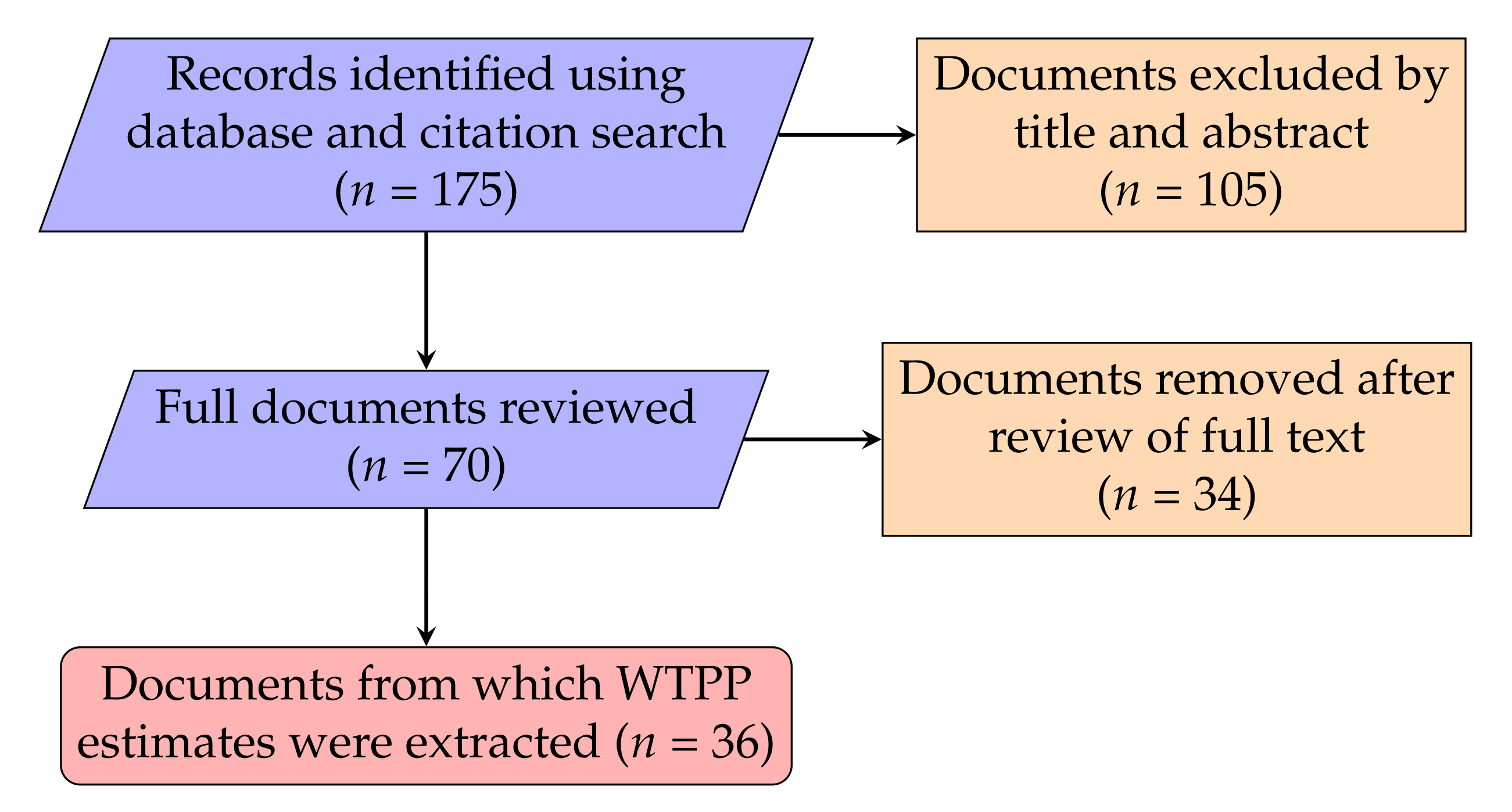
2.1. Collecting Papers

A combination of database and citation searching was used to gather the papers for inclusion in this analysis. For each search, titles were read, and the relevance was assessed. At this stage, papers were deemed relevant if their titles indicated that the study measured willingness-to-pay for fruits and/or vegetables. If there was any likelihood that the paper was relevant, the metadata (including abstract) was saved, and, where possible, the paper was downloaded. These search criteria are consistent with the guidelines for an economics meta-regression analysis [32,33,34]. The literature search method followed in this paper would be classified as a ’literature review’ rather than a ’systematic review’ [35].

Two sources were used for the database search: Google Scholar and EconLit [36]. EconLit is the standard database for searches in the economics literature [33]. Google Scholar is a complementary search tool [37] that has been used in recent reviews of willingness-to-pay for fruits and vegetables and other agricultural products [10,11,13,15]. Three Boolean search strings were used for the EconLit database: “(Willingness to pay OR WTP) AND producer AND fruit”, “(Willingness to pay OR WTP) AND producer AND vegetable, and “(Willingness to pay OR WTP) AND producer AND agriculture”.

Four Boolean search strings were used for searching Google Scholar: “Willingness to pay AND producer AND fruit”, “Willingness to pay AND producer AND vegetable, “Choice modeling AND producer AND fruit”, and “Choice modeling AND producer AND vegetable”. For Google Scholar searches, the first 10 pages of results were reviewed. All returned results from the EconLit database were reviewed. The database searches were performed on 7 December 2020. For both searches, papers were selected if they were published after 1990 and before the date of the search.

In addition, papers were identified using citation searching, also known as forwards and backward searching, i.e., reviewing the papers cited by several key papers as well as the papers that cite these key papers [38,39]. The citation searches were conducted in Fall, 2021. Four key papers were used for the citation search [7,8,30,40]. These papers were chosen on the basis of the authors’ knowledge of the literature at the beginning of the search process. The Lusk and Hudson [7] paper introduced the idea of using stated preference willingness-to-pay results in agribusiness decision making and is widely cited by both consumer and producer WTP studies.

The other three papers [8,30,40] emerged from the RosBREED project, a USDA funded interdisciplinary project to develop improved cultivars of rosaceous fruits and to estimate ex ante valuations of these improvements. At the time of the literature search, RosBREED was the first project the authors were aware of that sought to measure growers’ willingness-to-pay for fruits and vegetables.

Initially, 175 papers with titles that suggested they may be candidates for inclusion were identified. Only papers in English were considered for inclusion. The papers’ abstracts were screened for several characteristics: the use of a choice experiment, the measurement of willingness-to-pay for an agricultural product, or a focus on producers of specialty crops. If the abstracts were ambiguous, the content of the paper was skimmed for clarification.

This initial sample was screened to consider only studies that included data from the United States. Theoretical papers, conference posters, opinion pieces, and supply chain analyses were also discarded. Additionally, any papers that focused on non-crop agricultural products, such as meat, eggs, and dairy, were excluded. Published versions of dissertation chapters and theses were substituted where possible. If no published version was found, the original was kept.

This screening resulted in a set of 70 papers. After full text review, 34 papers were removed. The majority (26) were removed because their WTP estimates were derived from experimental auctions, rather than stated preference elicitation methods. The remaining eight papers were removed for a variety of reasons.

First, Yue et al. [41], which investigated breeders’ priorities, was excluded since the focus of this analysis is not on crop production technology providers. If this paper were included, other papers on production technology providers may also have to be included: irrigation, greenhouses, fertilizers, etc. In addition, Yue et al. [41] did not look at breeder trait priorities but rather the sources of information they used to set their trait priorities. This differentiates it from the other producer papers.

Second, Fernandez-Cornejo et al. [42] was excluded because it used revealed preference data rather than stated preferences. Third, a budget analysis paper, [43], was excluded, since it did not estimate WTP from consumers or producers directly.

Fourth, three papers [44,45,46] were excluded because they elicited respondent priorities, rather than a WTP estimates. Fifth, Chen et al. [47] was excluded because it measured grower WTP for biodegradable mulches and not fruits or vegetables. Finally, Guthman and Zurawski [48] was excluded because it elicited producer preferences through qualitative interviews.

After these rounds of review, 36 papers remained for inclusion in the analysis. Each of these papers used stated preference methods to produce a measure of WTP that could be converted into a percentage premium. Figure 1 shows the process followed to identify papers for inclusion in the meta-regression analysis.

Table A1. Papers providing WTPP estimates.

Paper	Year	Type	Crops	Group	Growing Method	Crop Type	Attributes	Study Type	Collect	Number of Measures	Measures	Number of WTPP Estimates	Number of Outliers
Blend and van Ravenswaay [19]	1999	JA	Apples	C	-	P	Credence	CA	C	2	D; PR	1	-
Bond et al. [73]	2008	JA	Potatoes; melons	C	O	A	Local; credence; multiple crops	CVM	S	1	PP	4	-
Campbell et al. [85]	2004	JA	Citrus	C	O	P	-	CA	I	1	D	4	-
Carpio and Isengildina-Massa [86]	2010	JA	Fruits; vegetables	C	-	-	Local	CVM	S	2	E; PP	3	-
Carroll et al. [51]	2013	JA	Tomatoes	C	O	A	Local; credence	CA	S	1	D	118	17
Chen et al. [87]	2019	JA	Strawberries	C	-	A	Credence	CVM	S	1	D	4	-
Choi et al. [21]	2017	JA	Strawberries	P	-	A	-	CA	S	1	D	12	2
Choi et al. [55]	2018	JA	Apples	P	-	P	-	CA	S	1	D	12	4
Coffey et al. [67]	2020	JA	Strawberries	P	-	A	Credence	CVM	I	1	D	3	-
Darby et al. [88]	2008	JA	Strawberries	C	-	A	Local; credence	CA	I	1	D	17	-
Ernst et al. [89]	2006	JA	Strawberries	C	O	A	Local; credence	CA; CVM	I	1	D	11	-
Gallardo and Wang [31]	2013	JA	Apples; pears	P	C	P	Credence	CA	I	1	D	40
Gallardo et al. [70]	2015	JA	Apples; cherries; peaches; strawberries	P	-	A and P	Multiple Crops	CA	I	1	D	24	12
Hu et al. [50]	2009	JA	Blueberries	C	-	P	Credence; processed	CA	I	1	D	42	9
Hu et al. [49]	2011	JA	Blueberries	C	-	P	Processed	CVM	I	1	D	15	1
Hu et al. [58]	2021	JA	Citrus	C	C	P	Credence; Processed	CA	S	2	D; PR	7	2
James et al. [90]	2009	JA	Apples	C	O	P	Credence; local; processed	CA	S	1	D	48	-
Jones and Brown [91]	2019	CP	Blueberries; citrus	C	C	P	Credence; processed	CA	S	1	PP	18	-
Li et al. [40]	2020	JA	Peaches	P	-	P	Credence	CA	S	1	D	5	1
Li et al. [59]	2020	JA	Strawberries	P	-	A	-	CA	S	1	D	5	1
Loureiro and Hine [92]	2002	JA	Potatoes	C	O	A	Credence; local	CVM	I	1	D	4	-
Loureiro et al. [93]	2002	JA	Apples	C	-	P	Credence	CA; CVM	I	2	D; PR	1	-
Markosyan et al. [94]	2009	JA	Apples	C	-	P	-	CVM	I	2	PP; PR	5	-
Meas et al. [57]	2014	JA	Blackberries	C	O	P	Credence; local; processed	CA	S	1	D	20	2
Oh et al. [95]	2015	JA	Apples; grapes	C	-	P	Credence; multiple crops	CA	S	2	D; PP	8	-
Onken et al. [72]	2011	JA	Strawberries	C	O	A	Credence; local; processed	CA	S	2	D; PP	120	-
[18]	2006	JA	Apples; bananas; leaf vegetables; broccoli	C	O and C	A and P	Credence; multiple crops	CA	S	2	D; PP	24	-
Sackett et al. [53]	2012	CP	Apples	C	O	P	Credence; local	CA	S	1	D	4	3
Teratanavat and Hooker [96]	2006	JA	Tomatoes	C	-	A	Credence; processed	CA	S	1	D	9	-
Thilmany et al. [97]	2008	JA	Melons	C	-	A	Credence; local	CVM	S	1	PP	20	-
Vassalos et al. [56]	2016	JA	Tomatoes	P	-	A	-	CA	S	2	D; PP	9	3
Wang et al. [98]	2017	JA	Strawberries	C	-	A	-	CA	S	1	PR	18	-
Xie et al. [52]	2016	JA	Broccoli	C	O and C	A	Credence	CA	S	1	D	15	6
Yue et al. [99]	2007	JA	Apples	C	O	P	-	CA	I	1	D	9	4
Yue et al. [8]	2017	JA	Apples; cherries; peaches; strawberries	P	-	A and P	Multiple Crops	CA	S	1	D	28	7
Zhao et al. [30]	2017	JA	Peaches	P	-	P	-	CA	S	1	D	10	2

Abbreviations: Column 3 (Type): JA = Journal Article, and CP = Conference Paper. Column 5 (Group): C = Consumers and P = Producers. Column 6 (Growing Method): - = Not Specified, O = Organic, and C = Conventional. Column 7 (Crop Type): A = Annual, and P = Perennial. Column 9 (Study Type): CA = Conjoint Analysis, and CVM = Contingent Valuation Method. Column 10 (Data Collection): S = Survey, I = Interview. Column 12 (Measures): D = Dollars, E = Elasticity, PP = Percent Premium, and PR = Probability.

in the appendix lists all included studies.

2.2. The Presence of Outliers and Their Removal

In total, there were 697 WTP estimates extracted from the data. The details of this process are outlined in Appendix A. In particular, Appendix A.1 explains the construction of the sample size for each estimate, Appendix A.2 includes details on merging the paper attributes and WTPP datasets, and Appendix A.3 contains methods for constructing WTP percentages for estimates not originally reported as percentages.

Outliers were defined as 1.5 times the interquartile range, which caused 76 WTP estimates to be excluded. Additionally, no calculable sample size was available for six observations, leaving 615 observations for use in the analysis. The two largest outliers came from [31]. In this study, apple and pear growers were asked what they were willing to pay per acre for chemical controls with reduced environmental impacts. Then, respondents were asked what they believed other growers were willing to pay for the same products.

The base price was given by industry experts to be around $35 per acre. While the direct valuation estimates were close to this base price, respondents estimated that other producers would be willing to pay between $100 and $350 per acre for the same products. Fifteen other papers contained outlying estimates [8,21,30,40,49,50,51,52,53,54,55,56,57,58,59].

2.3. Meta-Regression Analysis

Meta-regression analysis (MRA) is a form of meta-analysis that seeks to quantify how some outcome variable is affected by methods used in each paper included in the analysis, such as study design, data, and target population [33]. This technique has successfully been used to analyze WTP for food attributes, such as biofortification [12], health benefits [11], and local foods [13].

The percentage WTP (WTPP) was used as the summary statistic for the meta-regression analysis. This controls for differences in baseline prices among different crops, units of measurement, and between locations. The studies included in the analysis sought to calculate the marginal WTP for a variety of different product attributes, including experience and credence attributes. The common thread is that the respondent is asked about the WTP for a novel or hypothetical product. By combining these percent WTP estimates in the meta-regression analysis, the average percent WTP can be interpreted as the average WTP for novel or hypothetical produce. The percent premium was calculated using an equation adapted from Dolgopolova and Teuber [11]:

$$WTPP=\left(\frac{tWTP-P_{bench}}{P_{bench}}\right)\ast 100$$

(1)

where $tWTP$ is the total WTP (in dollars) for a given product and $P_{bench}$ is the benchmark or baseline price for the study.

The meta-regression analysis estimating equation is given by

$$WTP{P}_{ipt}={\beta }_1\sqrt{n_{ipt}}+{\beta }_{\mathbf{X}}{\mathbf{X}}_{ipt}+{\gamma }_t+{\epsilon }_{ipt}$$

(2)

where $WTP{P}_{ipt}$ is the percent premium WTP estimate i from paper p in year t, $\sqrt{n_{ipt}}$ is the square root of the sample size used to estimate $WTP{P}_{ipt}$, ${\beta }_1$ is a parameter to be estimated, ${\mathbf{X}}_{ipt}$ is a vector of independent explanatory variables listed in

Table 1. Independent variables for the meta-regression analysis.

Variable
$\sqrt{n}$	=The square root of the underlying study’s sample size
Producer	=1 if the sample group was producers
Survey	=1 if a survey was used to collect the data (baseline is interview)
WTP in Dollars	=1 if results were reported as WTP in dollars
Benchmark Price	=Price used for the product(s) evaluated
Local	=1 if product was locally grown
Organic	=1 if study product was organic
Processed	=1 if product was processed
Other Credence	=1 if WTP for a credence attribute not otherwise listed
	(health benefits, GM, sustainably produced, grown in US, or pesticide-free)

, ${\beta }_{\mathbf{X}}$ is a vector of parameters to be estimated, ${\gamma }_t$ are year-level fixed effects, and $\epsilon$ is a classical i.i.d error term.

In addition to the ability of meta-regression analysis to identify the effect of methodological choices on outcome variables, it can also uncover publication bias in a literature [60]. Publication bias occurs when researchers and editors are more likely to publish certain types of results over others, such as statistically significant results or results that are consistent with existing views [61].

Stanley [60] explained that the presence of publication bias creates a disadvantage for studies with small samples. These studies will have less statistical power and therefore less ability to find a significant effect compared to a larger study. Hence, they will need to search through more model specifications to find an effect large enough for publication. The presence of publication bias can be investigated by looking for evidence of an inverse relationship between sample size and effect size.

To test and control for potential publication bias, the square root of the study’s sample size is included in the MRA estimating equation. For MRAs on outcome variables that are combinations of the estimated regression coefficients, which is the case for percentage WTP estimates, Printezis et al. [13] note that the square root of the underlying study’s sample size is the most appropriate variable to control for publication bias. The reason is twofold. First, the inverse standard error of the WTP estimate (1/$SE$—the most commonly used variable to control for publication bias) is impossible to calculate given the reported data in many cases. Second, (1/$SE$) is an estimated value and subject to sampling error. The variable $\sqrt{n}$ is not subject to sampling error but is highly correlated with (1/$SE$).

A funnel plot, a common, informal tool for identifying the presence of publication bias [60], is not included in this analysis. A funnel plot indicates the absence of publication bias if the data points are symmetrically distributed around the most precise estimates, and its presence if the data are skewed. However, this assumes that there is a single true effect. Since this study combines studies examining the percentage WTP for a variety of effects, there are no a priori grounds for expecting a single, central estimate of percentage WTP. Instead, only the results of the Funnel Asymmetry Test (FAT) are included. The FAT indicates the presence of publication bias if $H_0$: ${\widehat{\beta }}_1=0$ in Equation (2) can be rejected [60]. Since this estimating equation controls for methodological differences between studies, including different effects of interest, the FAT is a more robust indicator of publication bias.

An important caveat is that rejection of the FAT’s null hypothesis is consistent with the presence of publication bias; however, there are other reasons why the hypothesis might be rejected, including true heterogeneity, and data irregularity [62]. A significantly negative value of ${\widehat{\beta }}_1$, meaning less precise estimates are likely to be larger, is more indicative of a bias towards publishing statistically significant results. On the other hand, a positive value of ${\widehat{\beta }}_1$ is unlikely to indicate a bias towards publishing statistically significant results and that an alternative reason is likely the cause of the asymmetry [63].

2.4. Alternative Regression Specifications

This analysis considers two alternative specifications of the model specified by Equation (2). The first specification includes only $\sqrt{n}$, a dummy variable indicating whether the study subjects were producers, and year fixed effects. A specification with only $\sqrt{n}$ and the producer dummy had a time trend in the residuals, which was controlled for by including the year fixed effects. The full specification includes the method variables and product attribute variables listed in Table 1. These additional variables account for methodological differences between the studies as well as differences in the types of good being studied.

In addition, the full model was estimated on two subsets of the data: a subset with only consumers and another with only producers. In the full model on the complete dataset, the specification allows consumers and producers to have different mean levels of WTPP but assumes that their marginal responses are identical, i.e., a one dollar increase in the baseline price would have the same effect on a consumer’s and a producer’s WTPP. Estimating the model on the two subsets allows the marginal responses to differ.

2.5. Controlling for Auto-Correlation and Heteroskedasticity

Each observed willingness-to-pay estimate is not drawn from an i.i.d distribution because multiple estimates are drawn from the same study. The estimates are clustered at the study level and, consequently, may have intra-study correlations. In addition, there may be intra-year correlations, even after the year fixed effects have been added to the model. These correlations may bias the estimated standard errors, making point estimates appear more precise than warranted. Indeed, there is evidence of auto-correlation (Appendix B.1) and heteroskedasticity (Appendix B.2) in several of the regression specifications.

To control for both of these issues, the standard errors were clustered at both the paper and year level [64]. Angrist and Pischke [65] suggest that the minimum number of clusters for robust inference is 42. This threshold is met for clustering at the paper level but not at the year level. Facing a similar problem, Printezis et al. [13] used wild bootstrapped standard errors as a robustness check, noting that it is well suited to meta-regression analysis. As a robustness check, the models in this analysis were also estimated with wild bootstrapped standard errors. The two-level clustered standard errors were calculated using the multiwayvcov package in R [66].

3. Results

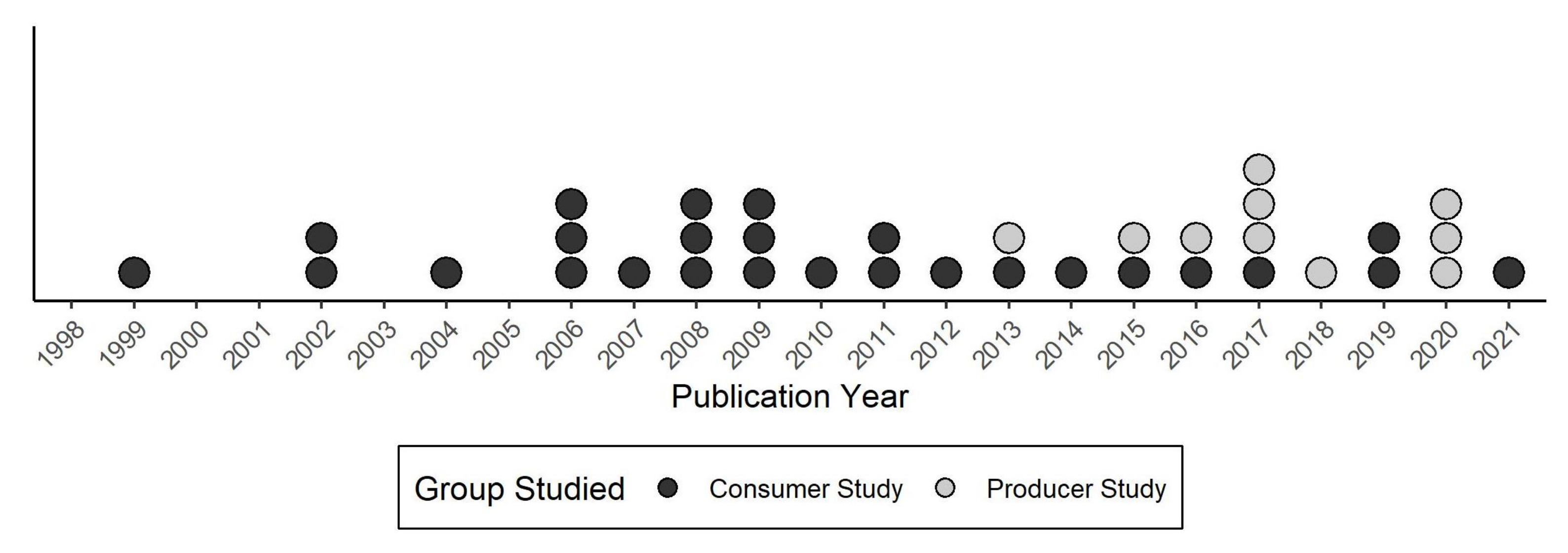
3.1. Paper Attributes

The umbrella category of “produce” encompasses a diverse range of crops whose cultivation and consumption vary widely. The column ’Crops’ in Table A1 lists the crops featured in the sample studies. Further, several studies considered processed food products, such as applesauce, alongside their fresh versions, while still others considered only the processed versions of a given crop.

Many studies sought to quantify preferences for particular credence attributes related to the origin or cultivation of particular goods.

Table 2. Summary of methods and attributes in included papers.

Key Variables	Full (N = 36)	Consumers (N = 26)	Producers (N = 10)
Study Type
CA	28	19	9
CVM	10	9	1
Data Collection Method
In-Person Survey (Interview)	12	9	3
Remote Survey	24	17	7
Results Measures
Dollar	29	19	10
Percent Premium	9	8	1
Elasticity	1	1	0
Probability of Purchase	5	5	0
Focus Attributes
Locally Grown	11	11	0
Organic	10	10	0
Processed Product	8	8	0
Other Credence	20	18	2
Rear Published
Min:	1999	1999	2013
Mean	2012	2010	2017
Max:	2021	2021	2020

presents tallies for the most common attributes studied in the sample. Counts in a section of this table need not add to N, as papers may have multiple attributes. For example, one producer paper reported both dollar and percent premium WTP measures [56].

There are few papers looking at fruit and vegetable producer adoption decisions. In this analysis, there were 26 papers that estimated the WTP of U.S. produce consumers for some crop or attribute but only 10 papers studying U.S. producers.

Three attributes were only applicable to consumers: locally grown, organic, and processed product. However, both consumers and producers were asked about their WTP for crops with a variety of credence attributes, such as non-GM or GM crops, the use of novel pest control technologies, preferences for sustainable cultivation practices, health benefits, or country of origin labeling. Consumers were asked about these attributes more frequently than producers.

Only one approach (whether in-person interview or mailed survey) was employed to collect data for all consumer and producer studies. In both groups, conjoint analysis was the most popular approach, used in 19 consumer studies and nine of the ten producer studies. Only one producer study used a CVM survey instrument [67].

It is important to consider that time may contribute to differences between consumer and producer studies: the popularity of certain methods or interest in certain topics normally ebb and flow as researchers’ understanding of these tools and phenomena evolve. In this analysis, producer studies were notably newer than the consumer studies, as Figure 2 demonstrates. Rounded to the nearest year, the mean consumer study was published in 2010, and the mean producer study was published in 2017.

3.2. Meta-Regression Analysis Results

Table 3. WTPP summary statistics.

Variable	Full (N = 615)	Consumers (N = 510)	Producers (N = 105)
WTP Premium (%)
Min.	−41.85	−41.85	−41.00
Max.	68.89	68.40	68.89
Mean	14.83	12.18	27.69
Sample Size (n)
Min.	13	56	13
Max.	8036	8036	321
Mean	683.87	809.87	71.85
Baseline Price
Min.	0.10	0.24	0.10
Max.	150.00	5.38	150.00
Mean	4.40	3.10	10.67
Year
Min.	1999	1999	2013
Max.	2021	2021	2020
Mean	2012	2011	2016
Methods Indicators (Means)
Survey	0.24	0.18	0.52
WTP in Dollars	0.89	0.86	1.00
Attributes Indicators (Means)
Local	0.25	0.30	0.00
Organic	0.18	0.21	0.00
Processed	0.43	0.52	0.00
Other Credence	0.33	0.36	0.15

summarizes the variables used in the meta-regression analysis of WTPP estimates. Several explanatory variables—WTP in Dollars, Local, Organic, Processed—have no variation for the producer studies, and thus they were dropped from the producer-only regression.

Table 4. Meta-regression results: comparing alternative models.

	Base	Full	Consumers	Producers
$\sqrt{n}$	$0.16$	0.28 *	0.26 *	−1.73 *
	$(-0.01;0.33)$	$(0.11;0.44)$	$(0.05;0.48)$	$(-2.73;-0.74)$
Producers	18.67 *	21.17 *
	$(7.17;30.18)$	$(14.61;27.73)$
Survey		−5.36	−12.51	0.57
		$(-15.57;4.86)$	$(-25.21;0.19)$	$(-0.33;1.47)$
WTP in Dollars		5.44	5.58
		$(-8.52;19.40)$	$(-12.38;23.53)$
Benchmark		−0.12 *	−4.49	−0.19 *
		$(-0.16;-0.09)$	$(-9.09;0.11)$	$(-0.19;-0.19)$
Local		24.79 *	28.39 *
		$(11.35;38.23)$	$(10.73;46.06)$
Organic		7.15	10.06
		$(-4.00;18.29)$	$(-4.58;24.70)$
Processed		5.96	12.17
		$(-7.83;19.76)$	$(-3.65;27.99)$
Other Credence		7.16	9.84	−21.76 *
		$(-2.99;17.31)$	$(-3.74;23.43)$	$(-21.95;-21.58)$
FE	Year	Year	Year	Year
Clustered SE	Year, Paper	Year, Paper	Year, Paper	Year, Paper
Bootstrap SE	No	No	No	No
Adj. R2	$0.46$	$0.55$	$0.49$	$0.73$
Num. obs.	615	615	510	105
F statistic	$26.29$	$27.75$	$19.84$	$29.62$

Numbers in parentheses are 95% confidence intervals. * Null hypothesis value outside the 95% confidence interval.

presents the results of the two regression specifications estimated on the complete dataset and the full specification estimated on only consumer or producer estimates. In the baseline model, the FAT null hypothesis cannot be rejected. However, the hypothesis of no relationship between sample size and WTPP is rejected at a 95 percent confidence level for the full, consumer-only, and producer-only models. In the full and consumer models, there is evidence of a positive relationship between the sample size and WTPP. This is unlikely to indicate the presence of publication bias [63].

These positive relationships in the base and consumer models are robust to the specification of the standard errors. Furthermore, when wild bootstrapped standard errors are used, the coefficients for $\sqrt{n}$ in the base models becomes significant at a 5 percent level (

Table A3. Meta-regression results: comparing alternative models with wild bootstrap standard errors.

	Base	Full	Consumers	Producers
$\sqrt{n}$	0.16 *	0.28 *	0.26 *	−1.73 *
	$(0.01;0.31)$	$(0.13;0.43)$	$(0.11;0.41)$	$(-2.37;-1.09)$
Producers	18.67 *	21.17 *
	$(7.26;30.09)$	$(9.66;32.68)$
Survey		−5.36	−12.51 *	0.57
		$(-11.59;0.87)$	$(-22.08;-2.93)$	$(-0.10;1.24)$
WTP in Dollars		5.44 *	5.58
		$(0.12;10.76)$	$(-2.55;13.71)$
Benchmark		−0.12	−4.49 *	−0.19 *
		$(-0.30;0.06)$	$(-7.82;-1.16)$	$(-0.19;-0.19)$
Local		24.79 *	28.39 *
		$(17.36;32.23)$	$(12.51;44.28)$
Organic		7.15 *	10.06
		$(1.83;12.46)$	$(-5.32;25.44)$
Processed		5.96	12.17 *
		$(-3.70;15.63)$	$(4.06;20.28)$
Other Credence		7.16	9.84	−21.76 *
		$(-1.25;15.56)$	$(-3.31;23.00)$	$(-21.97;-21.56)$
FE	Year	Year	Year	Year
Clustered SE	Year, Paper	Year, Paper	Year, Paper	Year, Paper
Bootstrap SE	Wild	Wild	Wild	Wild
Adj. R2	$0.46$	$0.55$	$0.49$	$0.73$
Num. obs.	615	615	510	105
F statistic	$26.29$	$27.75$	$19.84$	$29.62$

Numbers in parentheses are 95% confidence intervals. * Null hypothesis value outside the 95% confidence interval.

). In the producer-only model, the FAT null hypothesis is strongly rejected with a negative correlation between the sample size and WTPP. This is consistent with the presence of publication bias in this literature.

The significance of this estimate for the producer-only model is robust to the standard error specification, suggesting that the evidence showing statistically significant WTPP estimates are more likely to be selected for publication is not an artefact of the variance-covariance matrix estimation procedure. In addition, including $\sqrt{n}$ in the regression specification also controls for any potential publication bias that varies systematically with the WTPP estimate’s precision, removing this bias from the estimates of the other variables.

The estimate of the producers dummy variable in the base specification indicates that WTPP estimates are 18.67 percentage points higher when producers are studied, compared to consumers, after controlling for year fixed effects, and correlation between sample size and WTPP. This result is robust when controlling for differences in methods and product attributes—increasing only slightly to 21.17 percent in the full specification. The 95 percent confidence interval is reported under each coefficient estimate in Table 4 to emphasize the range of likely estimate values [68,69]. The 95 percent confidence interval for the producers dummy in the full specification is 14.61 to 27.73 percent.

The majority of method and attribute variables are not significantly different from zero. In the full and producer-only models, the data collection method did not impact the estimated WTPP. However, in the consumer-only model, estimates collected by surveys had a 12.51 percent lower WTPP than estimates from in-person interviews. However, this estimate is only significant with bootstrapped standard errors.

In each specification, an increase in the baseline price decreased the WTPP. In the full dataset, a $1 increase in the baseline price would reduce the WTPP by 0.12 percentage points. This result was similar for the producer-only model with a 0.19 percent decrease in WTPP per dollar increase. The effect was larger in the consumer-only model, where a $1 increase in the baseline price would decrease the WTPP by 4.49 percentage points; however, this was not robust to standard error specification. Part of this sensitivity can be explained by the different ranges in baseline prices between producers and consumers. Consumer prices range from $0.24 to $5.38, while producer prices range from $0.10 to $150.

In the full and consumer-only models, the presence of a credence attribute (other than local, organic, or processed) had no significant impact on WTPP. On the other hand, the presence of this variable presence decreased WTPP for producers by 21.76 percentage points. Finally, the presence of a local attribute increased WTPP by 24.79 percentage points in the full model. When excluding producers, this effect increased to 28.39 percentage points. There was insufficient variation of this variable in the producer-only sample, and thus it was excluded from the producer-only regression.

4. Discussion and Conclusions

For a new crop to be successfully adopted by consumers, it must first be adopted by producers. This study aimed to identify whether producers’ WTP for novel or hypothetical fruits and vegetables was different than for consumers. The results of this meta-regression analysis showed that producers were, on average, willing to pay about 20 percentage points more for novel or hypothetical products.

This result suggests that a product developer who estimates a consumer WTP high enough to justify developing the product, would, all else being equal, find producers also willing to adopt it. This finding is consistent with the meta-analysis by Olum et al. [14], who found that agricultural producers generally have a high WTP for novel practices and technologies. This makes intuitive sense as well, since the producers may capture a share of the potential returns to the new product. However, these results do not imply the converse; that is, if producers are likely to adopt the new product, it does not necessarily imply that consumers also will.

The meta-regression analysis found that method and product attributes affected WTPP. Consumer estimates were approximately 14 percentage points lower when respondents answered a survey compared to an in-person interview. On the other hand, the elicitation method had no measurable impact on producer answers. Consumers were willing to pay, on average, 30 percentage points more for locally grown produce.

This is broadly consistent with the findings of Printezis et al. [13] whose meta-regression analysis found consumers were willing to pay an average 41 to 52 percentage point premium for local produce, animal, and processed foods and found that the WTP for produce was lower than for animal or processed foods. These results were also consistent with previous findings in consumer-focused meta-analyses, which found that consumers were willing to pay high premiums for produce with credence attributes, such as organic, non-GM, or locally-grown [9,10,11].

This study compared consumer and producer WTP in general. There were two studies included in this analysis that compared producer and consumer preferences for the same crop. Choi et al. [55] compared producer and consumer preferences for six apple attributes. They found the mean consumer willingness-to-pay for appearance and crispness was higher than for producers and that the other four attributes were not statistically significantly different between producers and consumers.

Choi et al. [21] did not find a statistically significant difference between producer and consumer WTP for strawberry attributes. Since the direct, literal apples-to-apples comparison found that consumer WTP was either higher or the same as producer WTP, it is possible that the results in this analysis are driven by differences across crops. As more producer WTP studies are conducted, future meta-regression analyses may be able to better control for the particular crops being studied.

The study of fruit and vegetable producer WTP is relatively new, and there are far fewer studies in this field. This led to a relative lack of variation or availability in many of the methodological and attribute variables that were available for consumer estimates, preventing these variables from being used as controls. Therefore, unobserved variable bias may be present in the results; this bias could be reduced as additional producer studies are published.

The studies included in this analysis were restricted to the United States. As this is the first paper (to the authors’ knowledge) to directly compare the preferences of produce consumers and producers, restricting attention to one country reduces possible sources of difference attributable to culture. This context is quite distinct from Low- and Middle-Income Countries (LMICs), where producer preferences may be driven by different constraints and needs (e.g., subsistence farmers).

The EU is a natural point of comparison; however, the policies that govern agricultural production are quite distinct and, because they are determined at the continental level, may not directly reflect the preferences of the consumers to whom these goods are marketed. Future research could consider how these differences play out in other cultural contexts, or how stable these results might be when broadening the lens to a multi-cultural or cross-country sample.

Several existing reviews that included producer or consumer WTP for produce disaggregate the results by geographical region. These reviews give clues to the expected results of applying this study’s methodology to other geographical regions. The determinants of producer or consumer WTP depend on the region and the particular product attributes studied [2,15]. Sociodemographic factors were less important in explaining producer WTP in high-income countries, relative to LMICs [14]. Further, results were mixed for consumer willingness-to-pay by region and depended on the particular attribute being studied.

Printezis et al. [13] found U.S. consumers willing to pay an additional 42 percent for local products compared to consumers in European countries, the Republic of Dominica, and Australia. Dolgopolova and Teuber [11] found no significant differences in WTP for health benefits in foods between consumers in the U.S., Europe, and other regions. De Steur et al. [12] found consumers in LMICs willing to pay on average 25.38 percent more for bio-fortified foods. These results suggest that the magnitude of the difference between consumer and producer WTP in other geographical regions is an empirical question and will depend on the types of product attributes studied in other regions.

An additional limitation is the method used to collect the studies for the analysis, which limits its replicability and scope. First, the use of Google Scholar limits the replicability of the analysis. Google Scholar search results for an identical string can change depending on the search time and location [37]. Gusenbauer and Haddaway [37] recommended that Google Scholar only be used as a supplementary search method. However, they found that EconLit was suitable as a primary search tool. Second, the use of only two search tools, EconLit and Google Scholar, means that the search cannot be considered systematic. Therefore, there may be additional eligible studies that were not captured and included in this analysis.

The meta-regression analysis found evidence consistent with publication bias in the producer studies, suggesting that studies with a significant result were more likely to be published and that the true producer willingness-to-pay may be lower than reported. The meta-regression analysis controls for the bias that is directly proportional to the square root of the sample size; however, the result would be more robust with an unbiased set of WTPP estimates, which may be achieved by a broader literature search, or as more producer papers are published.

An issue that may potentially make the estimation of producers’ WTP less accurate is the difference in decision making contexts between producers and consumers. Ex post studies of technological adoption have long been a mainstay of agricultural economics research; however, this analysis indicates that measuring fruit and vegetable producer valuation ex ante using stated preference methods is relatively new. These studies used established methods of measuring consumer preferences for novel food products.

The approaches developed for ex ante evaluation of consumer purchase behavior, particularly for fruits and vegetables, center around small, routine purchases for final consumption—for example, the choice between alternative types of apples considered for a few moments at the grocery store. On the other hand, when producers consider adopting a new crop or process, they must choose from many more input combinations (such as cultivars, production systems, and marketing channels) over a much longer horizon (at least a season). These decisions must be made in a context subject to substantial risk.

A survey asking a producer to make this hypothetical decision in a short time-frame may not accurately reflect the decision they would make if they engaged in their normal decision-making process. Without further study, it is unclear if this would systematically bias producer WTPP estimates upwards or downwards; however, it is likely that it would increase the variance of estimated WTPP relative to consumers.

The results of this analysis provide initial evidence that U.S. producers of fruits and vegetables are generally willing to pay a higher premium for novel or hypothetical produce compared to U.S. consumers. The results from this study suggest there is value in additional research into using consumer willingness-to-pay measurements to predict producer adoption decisions, especially since methods to measure consumer WTP are more established, and consumer WTP estimates are more common.

References

1. Louviere, J.J.; Hensher, D.A.; Swait, J.D.; Adamowicz, W. Stated Choice Methods: Analysis and Applications; Cambridge University Press: Cambridge, UK, 2000. [Google Scholar]
2. Moser, R.; Raffaelli, R.; Thilmany, D.D. Consumer Preferences for Fruit and Vegetables with Credence-Based Attributes: A Review. Int. Food Agribus. Manag. Rev. 2011, 14, 121–142. [Google Scholar]
3. Yencho, G.C.; Pecota, K.V.; Schultheis, J.R.; VanEsbroeck, Z.P.; Holmes, G.J.; Little, B.E.; Thornton, A.C.; Truong, V.D. ’Covington’ Sweetpotato. HortScience 2008, 43, 1911–1914. [Google Scholar] [CrossRef] [Green Version]
4. Evans, K.M.; Barritt, B.H.; Konishi, B.S.; Brutcher, L.J.; Ross, C.F. ’WA 38’ Apple. HortScience 2012, 47, 1177–1179. [Google Scholar] [CrossRef] [Green Version]
5. Luby, J.J.; Bedford, D.S. Cultivars as Consumer Brands: Trends in Protecting and Commercializing Apple Cultivars via Intellectual Property Rights. Crop Sci. 2015, 55, 2504–2510. [Google Scholar] [CrossRef]
6. Katz, B. Meet ’Cosmic Crisp’, a New Hybrid Apple That Stays Fresh for a Year. Smithsonian Magazine, 4 December 2019. [Google Scholar]
7. Lusk, J.L.; Hudson, D. Willingness-to-Pay Estimates and Their Relevance to Agribusiness Decision Making. Rev. Agric. Econ. 2004, 26, 152–169. [Google Scholar] [CrossRef]
8. Yue, C.; Zhao, S.; Gallardo, K.; McCracken, V.; Luby, J.; McFerson, J.U.S. Growers’ Willingness to Pay for Improvement in Rosaceous Fruit Traits. Agric. Resour. Econ. Rev. 2017, 46, 103–122. [Google Scholar] [CrossRef] [Green Version]
9. Boccaletti, S. Environmentally Responsible Food Choice. OECD J. Gen. Pap. 2008, 2008, 117–152. [Google Scholar] [CrossRef]
10. Cecchini, L.; Torquati, B.; Chiorri, M. Sustainable Agri-Food Products: A Review of Consumer Preference Studies through Experimental Economics. Agric. Econ. Czech 2018, 64, 554–565. [Google Scholar] [CrossRef]
11. Dolgopolova, I.; Teuber, R. Consumers’ Willingness to Pay for Health Benefits in Food Products: A Meta-Analysis. Appl. Econ. Perspect. Policy 2018, 40, 333–352. [Google Scholar] [CrossRef]
12. De Steur, H.; Wesana, J.; Blancquaert, D.; Van Der Straeten, D.; Gellynck, X. Methods Matter: A Meta-Regression on the Determinants of Willingness-to-Pay Studies on Biofortified Foods. Ann. N. Y. Acad. Sci. 2016, 1290, 34–46. [Google Scholar] [CrossRef] [Green Version]
13. Printezis, I.; Grebitus, C.; Hirsch, S. The Price Is Right!? A Meta-Regression Analysis on Willingness to Pay for Local Food. PLoS ONE 2019, 14, e0215847. [Google Scholar] [CrossRef] [Green Version]
14. Olum, S.; Gellynck, X.; Juvinal, J.; Ongeng, D.; De Steur, H. Farmers’ Adoption of Agricultural Innovations: A Systematic Review on Willingness to Pay Studies. Outlook Agric. 2020, 49, 187–203. [Google Scholar] [CrossRef]
15. Mamine, F.; Fares, M.; Minviel, J.J. Contract Design for Adoption of Agrienvironmental Practices: A Meta-analysis of Discrete Choice Experiments. Ecol. Econ. 2020, 176, 12. [Google Scholar] [CrossRef]
16. Vecchio, R.; Borrello, M. Measuring Food Preferences through Experimental Auctions: A Review. Food Res. Int. 2019, 116, 1113–1120. [Google Scholar] [CrossRef]
17. Rosen, S. Hedonic Prices and Implicit Markets: Product Differentiation in Pure Competition. J. Political Econ. 1974, 82, 34–55. [Google Scholar] [CrossRef]
18. Onozaka, Y.; Bunch, D.; Larson, D. What Exactly Are They Paying For? Explaining the Price Premium for Organic Fresh Produce. Update Agric. Resour. Econ. 2006, 9, 2–4. [Google Scholar]
19. Blend, J.R.; van Ravenswaay, E.O. Measuring Consumer Demand for Ecolabeled Apples. Am. J. Agric. Econ. 1999, 81, 1072–1077. [Google Scholar] [CrossRef]
20. Bernard, J.C.; Bernard, D.J. Comparing Parts with the Whole: Willingness to Pay for Pesticide-Free, Non-GM, and Organic Potatoes and Sweet Corn. J. Agric. Resour. Econ. 2010, 35, 457–475. [Google Scholar]
21. Choi, J.W.; Yue, C.; Luby, J.; Zhao, S.; Gallardo, K.; McCracken, V.; McFerson, J. Estimating Strawberry Attributes’ Market Equilibrium Values. HortScience 2017, 52, 742–748. [Google Scholar] [CrossRef] [Green Version]
22. Johnston, R.J.; Boyle, K.J.; Adamowicz, W.V.; Bennett, J.; Brouwer, R.; Cameron, T.A.; Hanemann, W.M.; Hanley, N.; Ryan, M.; Scarpa, R.; et al. Contemporary Guidance for Stated Preference Studies. J. Assoc. Environ. Resour. Econ. 2017, 4, 319–405. [Google Scholar] [CrossRef] [Green Version]
23. Lusk, J.L. Experimental Auctions for Marketing Applications: A Discussion. J. Agric. Appl. Econ. 2003, 35, 349–360. [Google Scholar] [CrossRef]
24. Street, D.J.; Burgess, L. Typical Stated Choice Experiments. In The Construction of Optimal Stated Choice Experiments: Theory and Methods; Street, D.J., Burgess, L., Eds.; Wiley Series in Probability and Statistics; John Wiley & Sons: Hoboken, NJ, USA, 2007; pp. 1–13. [Google Scholar]
25. McFadden, D. The Measurement of Urban Travel Demand. J. Public Econ. 1974, 3, 303–328. [Google Scholar] [CrossRef]
26. Lloyd-Smith, P.; Zawojska, E.; Adamowicz, W.L. Is There Really a Difference between “Contingent Valuation” and “Choice Experiments”? In Proceedings of the American Agricultural and Applied Economics Association Annual Meeting, Washington, DC, USA, 5–7 August 2018; p. 36. [Google Scholar]
27. Orme, B.K. Getting Started with Conjoint Analysis: Strategies for Product Design and Pricing Research; Research Publishers, LLC: Madison, WI, USA, 2006. [Google Scholar]
28. Johnson, F.R.; Kanninen, B.; Bingham, M.; Ozdemir, S. Experimental Design for Stated Choice Studies. In Valuing Environmental Amenities Using Stated Choice Studies: A Common Sense Approach to Theory and Practice; Kanninen, B., Ed.; The Economics of Non-Market Goods and Resources; Springer: Dordecht, The Netherlands, 2007; pp. 159–202. [Google Scholar]
29. Alberini, A.; Longo, A.; Veronesi, M. Basic Statistical Models for Stated Choice Studies. In Valuing Environmental Amenities Using Stated Choice Studies: A Common Sense Approach to Theory and Practice; The Economics of Non-Market Goods and Resources; Springer: Dordecht, The Netherlands, 2007; pp. 203–227. [Google Scholar]
30. Zhao, S.; Yue, C.; Luby, J.; Gallardo, K.; McCracken, V.; McFerson, J.; Layne, D.R.U.S. Peach Producer Preference and Willingness to Pay for Fruit Attributes. HortScience 2017, 52, 116–121. [Google Scholar] [CrossRef] [Green Version]
31. Gallardo, R.K.; Wang, Q. Willingness to Pay for Pesticides’ Environmental Features and Social Desirability Bias: The Case of Apple and Pear Growers. J. Agric. Resour. Econ. 2013, 38, 124–139. [Google Scholar]
32. Stanley, T.D.; Jarrell, S.B. Meta-Regression Analysis: A Quantitative Method of Literature Surveys. J. Econ. Surv. 1989, 3, 161–170. [Google Scholar] [CrossRef]
33. Stanley, T.D. Wheat From Chaff: Meta-Analysis as Quantitative Literature Review. J. Econ. Perspect. 2001, 15, 131–150. [Google Scholar] [CrossRef]
34. Stanley, T.; Doucouliagos, H.; Giles, M.; Heckemeyer, J.H.; Johnston, R.J.; Laroche, P.; Nelson, J.P.; Paldam, M.; Poot, J.; Pugh, G.; et al. Meta-Analysis of Economics Research Reporting Guidelines. J. Econ. Surv. 2013, 27, 390–394. [Google Scholar] [CrossRef]
35. Grant, M.J.; Booth, A. A Typology of Reviews: An Analysis of 14 Review Types and Associated Methodologies. Health Inf. Libr. J. 2009, 26, 91–108. [Google Scholar] [CrossRef]
36. Machi, L.A.; McEvoy, B.T. The Literature Review: Six Steps to Success; Corwin Press: Thousand Oaks, CA, USA, 2012. [Google Scholar]
37. Gusenbauer, M.; Haddaway, N.R. Which Academic Search Systems Are Suitable for Systematic Reviews or Meta-Analyses? Evaluating Retrieval Qualities of Google Scholar, PubMed, and 26 Other Resources. Res. Synth. Methods 2020, 11, 181–217. [Google Scholar] [CrossRef] [Green Version]
38. Briscoe, S.; Bethel, A.; Rogers, M. Conduct and Reporting of Citation Searching in Cochrane Systematic Reviews: A Cross-Sectional Study. Res. Synth. Methods 2020, 11, 169–180. [Google Scholar] [CrossRef]
39. Wright, K.; Golder, S.; Rodriguez-Lopez, R. Citation Searching: A Systematic Review Case Study of Multiple Risk Behaviour Interventions. BMC Med. Res. Methodol. 2014, 14, 73. [Google Scholar] [CrossRef] [Green Version]
40. Li, Z.; Gallardo, R.K.; McCracken, V.; Yue, C.; Whitaker, V.; McFerson, J.R. Grower Willingness to Pay for Fruit Quality versus Plant Disease Resistance and Welfare Implications: The Case of Florida Strawberry. J. Agric. Resour. Econ. 2020, 45, 199–218. [Google Scholar] [CrossRef]
41. Yue, C.; Gallardo, R.K.; McCracken, V.A.; Luby, J.; McFerson, J.R.; Liu, L.; Iezzoni, A. Technical and Socioeconomic Challenges to Setting and Implementing Priorities in North American Rosaceous Fruit Breeding Programs. HortScience 2012, 47, 1320–1327. [Google Scholar] [CrossRef]
42. Fernandez-Cornejo, J.; Beach, E.D.; Huang, W.Y. The Adoption of Integrated Pest Management Technologies by Vegetable Growers; Technical Report 1486-2018-6697; United States Department of Agriculture (USDA): Washington, DC, USA, 1992. [CrossRef]
43. Barrett, C.E.; Zhao, X.; Hodges, A.W. Cost Benefit Analysis of Using Grafted Transplants for Root-knot Nematode Management in Organic Heirloom Tomato Production. HortTechnology 2012, 22, 252–257. [Google Scholar] [CrossRef] [Green Version]
44. Gallardo, R.K.; Stafne, E.T.; DeVetter, L.W.; Zhang, Q.; Li, C.; Takeda, F.; Williamson, J.; Yang, W.Q.; Cline, W.O.; Beaudry, R.; et al. Blueberry Producers’ Attitudes toward Harvest Mechanization for Fresh Market. HortTechnology 2018, 28, 10–16. [Google Scholar] [CrossRef] [Green Version]
45. Gallardo, R.K.; Klingthong, P.; Zhang, Q.; Polashock, J.; Atucha, A.; Zalapa, J.; Rodriguez-Saona, C.; Vorsa, N.; Iorizzo, M. Breeding Trait Priorities of the Cranberry Industry in the United States and Canada. HortScience 2018, 53, 1467–1474. [Google Scholar] [CrossRef] [Green Version]
46. Dentoni, D.; Tonsor, G.T.; Calantone, R.; Peterson, H.C. Brand Coopetition with Geographical Indications: Which Information Does Lead to Brand Differentiation? New Medit 2013, 12, 14–27. [Google Scholar]
47. Chen, K.J.; Galinato, S.P.; Marsh, T.L.; Tozer, P.R.; Chouinard, H.H. Willingness to Pay for Attributes of Biodegradable Plastic Mulches in the Agricultural Sector. HortTechnology 2020, 30, 437–447. [Google Scholar] [CrossRef]
48. Guthman, J.; Zurawski, E. “If I Need to Put More Armor on, I Can’t Carry More Guns”: The Collective Action Problem of Breeding for Productivity in the California Strawberry Industry. Int. J. Sociol. Agric. Food 2020, 26, 69–88. [Google Scholar] [CrossRef]
49. Hu, W.; Woods, T.A.; Bastin, S.; Cox, L.J.; You, W. Assessing Consumer Willingness to Pay for Value-Added Blueberry Products Using a Payment Card Survey. J. Agric. Appl. Econ. 2011, 43, 243–258. [Google Scholar] [CrossRef] [Green Version]
50. Hu, W.; Woods, T.A.; Bastin, S. Consumer Acceptance and Willingness to Pay for Blueberry Products with Nonconventional Attributes. J. Agric. Appl. Econ. 2009, 41, 47–69. [Google Scholar] [CrossRef] [Green Version]
51. Carroll, K.A.; Bernard, J.C.; Pesek, J.D. Consumer Preferences for Tomatoes: The Influence of Local, Organic, and State Program Promotions by Purchasing Venue. J. Agric. Resour. Econ. 2013, 38, 379–396. [Google Scholar]
52. Xie, J.; Gao, Z.; Swisher, M.; Zhao, X. Consumers’ Preferences for Fresh Broccolis: Interactive Effects between Country of Origin and Organic Labels. Agric. Econ. 2016, 47, 181–191. [Google Scholar] [CrossRef]
53. Sackett, H.M.; Shupp, R.S.; Tonsor, G.T. Discrete Choice Modeling of Consumer Preferences for Sustainably Produced Steak and Apples. In Proceedings of the 2012 AAEA/EAAE Food Environment Symposium, Boston, MA, USA, 30–31 May2012. [Google Scholar]
54. Yue, C.; Jensen, H.H.; Mueller, D.S.; Nonnecke, G.R.; Gleason, M.L. Assessing Consumers’ Valuation of Cosmetically Damaged Apples Using a Mixed Probit Model; Iowa State University: Ames, IA, USA, 2005; p. 24. [Google Scholar]
55. Choi, J.W.; Yue, C.; Luby, J.; Zhao, S.; Gallardo, K.; McCracken, V.; McFerson, J. Estimation of Market Equilibrium Values for Apple Attributes. China Agric. Econ. Rev. 2018, 10, 135–151. [Google Scholar] [CrossRef]
56. Vassalos, M.; Hu, W.; Woods, T.; Schieffer, J.; Dillon, C. Risk Preferences, Transaction Costs, and Choice of Marketing Contracts: Evidence from a Choice Experiment with Fresh Vegetable Producers. Agribusiness 2016, 32, 379–396. [Google Scholar] [CrossRef]
57. Meas, T.; Hu, W.; Batte, M.T.; Woods, T.A.; Ernst, S. Substitutes or Complements? Consumer Preference for Local and Organic Food Attributes. Am. J. Agric. Econ. 2014, 97, 1044–1071. [Google Scholar] [CrossRef]
58. Hu, Y.; House, L.A.; McFadden, B.R.; Gao, Z. The Influence of Choice Context on Consumers’ Preference for GM Orange Juice. J. Agric. Econ. 2021, 72, 547–563. [Google Scholar] [CrossRef]
59. Li, Z.; Gallardo, R.K.; McCracken, V.A.; Yue, C.; Gasic, K.; Reighard, G.; McFerson, J.R.U.S. Southeastern Peach Growers Preferences for Fruit Size and External Color versus Resistance to Brown Rot Disease. HortTechnology 2020, 30, 576–584. [Google Scholar] [CrossRef]
60. Stanley, T.D. Beyond Publication Bias. J. Econ. Surv. 2005, 19, 309–345. [Google Scholar] [CrossRef]
61. Card, D.; Krueger, A.B. Time-Series Minimum-Wage Studies: A Meta-analysis. Am. Econ. Rev. 1995, 85, 238–243. [Google Scholar]
62. Egger, M.; Smith, G.D.; Schneider, M.; Minder, C. Bias in Meta-Analysis Detected by a Simple, Graphical Test. BMJ 1997, 315, 629–634. [Google Scholar] [CrossRef] [Green Version]
63. Sterne, J.A.C.; Sutton, A.J.; Ioannidis, J.P.A.; Terrin, N.; Jones, D.R.; Lau, J.; Carpenter, J.; Rucker, G.; Harbord, R.M.; Schmid, C.H.; et al. Recommendations for Examining and Interpreting Funnel Plot Asymmetry in Meta-Analyses of Randomised Controlled Trials. BMJ 2011, 343, d4002. [Google Scholar] [CrossRef] [Green Version]
64. Cheah, B.C. Clustering Standard Errors or Modeling Multilevel Data; University of Columbia: New York, NY, USA, 2009. [Google Scholar]
65. Angrist, J.D.; Pischke, J.S. Mostly Harmless Econometrics: An Empiricist’s Companion; Princeton University Press: Princeton, NJ, USA, 2009. [Google Scholar]
66. Graham, N.; Arai, M.; Hagströmer, B. Multiwayvcov: Multi-Way Standard Error Clustering. R Package Version 1.2.3. 2016. Available online: https://CRAN.R-project.org/package=multiwayvcov (accessed on 8 February 2022).
67. Coffey, B.; Trinetta, V.; Nwadike, L.; Yucel, U. Producer Willingness to Pay for Enhanced Packaging to Prevent Postharvest Decay of Strawberries. J. Appl. Farm Econ. 2020, 3, 30–41. [Google Scholar] [CrossRef]
68. Romer, D. In Praise of Confidence Intervals. AEA Pap. Proc. 2020, 110, 55–60. [Google Scholar] [CrossRef]
69. Imbens, G.W. Statistical Significance, p-Values, and the Reporting of Uncertainty. J. Econ. Perspect. 2021, 35, 157–174. [Google Scholar] [CrossRef]
70. Gallardo, R.K.; Li, H.; McCracken, V.; Yue, C.; Luby, J.; McFerson, J.R. Market Intermediaries’ Willingness to Pay for Apple, Peach, Cherry, and Strawberry Quality Attributes. Agribusiness 2015, 31, 259–280. [Google Scholar] [CrossRef]
71. Silva, A.; Nayga, R.M.; Campbell, B.L.; Park, J.L. On the Use of Valuation Mechanisms to Measure Consumers’ Willingness to Pay for Novel Products: A Comparison of Hypothetical and Non-Hypothetical Values. Int. Food Agribus. Manag. Rev. 2007, 10, 165–180. [Google Scholar] [CrossRef]
72. Onken, K.A.; Bernard, J.C.; Pesek, J.D. Comparing Willingness to Pay for Organic, Natural, Locally Grown, and State Marketing Program Promoted Foods in the Mid-Atlantic Region. Agric. Resour. Econ. Rev. 2011, 40, 33–47. [Google Scholar] [CrossRef]
73. Bond, C.A.; Thilmany, D.D.; Keeling Bond, J. Understanding Consumer Interest in Product and Process-Based Attributes for Fresh Produce. Agribusiness 2008, 24, 231–252. [Google Scholar] [CrossRef]
74. Evans, E.A.; Ballen, F.H.; De Oleo, B.; Crane, J.H. Willingness of South Florida Fruit Growers to Adopt Genetically Modified Papaya: An Ex-ante Evaluation. AgBioForum 2017, 20, 156–162. [Google Scholar]
75. Gifford, K.; Bernard, J.C. Factor and Cluster Analysis of Willingness to Pay for Organic and Non-GM Food. J. Food Distrib. Res. 2008, 39, 26–39. [Google Scholar] [CrossRef]
76. Govindasamy, R.; Arumugam, S.; Vellangany, I.; Ozkan, B. Willingness to Pay a High-Premium for Fresh Organic Produce: An Econometric Analysis. Agric. Econ. Res. Rev. 2018, 31, 45. [Google Scholar] [CrossRef] [Green Version]
77. Govindasamy, R.; Italia, J. Willingness-to-Purchase Comparison of Integrated Pest Management and Conventional Produce. Agribusiness 1998, 4, 403–414. [Google Scholar] [CrossRef]
78. Hamilton, S.F.; Sunding, D.L.; Zilberman, D. Public Goods and the Value of Product Quality Regulations: The Case of Food Safety. J. Public Econ. 2003, 87, 799–817. [Google Scholar] [CrossRef] [Green Version]
79. Lagoudakis, A.; McKendree, M.G.; Malone, T.; Caputo, V. Incorporating Producer Opinions into a SWOT Analysis of the U.S. Tart Cherry Industry. Int. Food Agribus. Manag. Rev. 2020, 23, 547–561. [Google Scholar] [CrossRef]
80. Loureiro, M.L.; McCluskey, J.J.; Mittelhammer, R.C. Assessing Consumer Preferences for Organic, Eco-labeled, and Regular Apples. J. Agric. Resour. Econ. 2001, 26, 404–416. [Google Scholar]
81. Nelson, M.C.; Styles, E.K.; Pattanaik, N.; Liu, X.; Brown, J. Georgia Farmers’ Perceptions of Production Barrier in Organic Vegetable and Fruit Agriculture. In Proceedings of the 2015 Southern Agricultural Economics Association Annual Meeting, Atlanta, GA, USA, 31 January–3 February 2015. [Google Scholar] [CrossRef]
82. Yu, H.; Neal, J.A.; Sirsat, S.A. Consumers’ Food Safety Risk Perceptions and Willingness to Pay for Fresh-Cut Produce with Lower Risk of Foodborne Illness. Food Control 2018, 86, 83–89. [Google Scholar] [CrossRef]
83. Yue, C.; Gallardo, R.K.; Luby, J.J.; Rihn, A.L.; McFerson, J.R.; McCracken, V.; Gradziel, T.; Gasic, K.; Reighard, G.L.; Clark, J.; et al. An Evaluation of U.S. Peach Producers’ Trait Prioritization: Evidence from Audience Surveys. HortScience 2014, 49, 1309–1314. [Google Scholar] [CrossRef]
84. Yue, C.; Gallardo, R.K.; Luby, J.; Rihn, A.; McFerson, J.R.; McCracken, V.; Whitaker, V.M.; Finn, C.E.; Hancock, J.F.; Weebadde, C.; et al. An Evaluation of U.S. Strawberry Producers Trait Prioritization: Evidence from Audience Surveys. HortScience 2014, 49, 188–193. [Google Scholar] [CrossRef] [Green Version]
85. Campbell, B.L.; Nelson, R.G.; Ebel, R.C.; Dozier, W.A.; Adrian, J.L.; Hockema, B.R. Fruit Quality Characteristics That Affect Consumer Preferences for Satsuma Mandarins. HortScience 2004, 39, 1664–1669. [Google Scholar] [CrossRef]
86. Carpio, C.E.; Isengildina-Massa, O. To Fund or Not to Fund: Assessment of the Potential Impact of a Regional Promotion Campaign. J. Agric. Resour. Econ. 2010, 35, 245–260. [Google Scholar]
87. Chen, K.J.; Marsh, T.L.; Tozer, P.R.; Galinato, S.P. Biotechnology to Sustainability: Consumer Preferences for Food Products Grown on Biodegradable Mulches. Food Res. Int. 2019, 116, 200–210. [Google Scholar] [CrossRef] [PubMed]
88. Darby, K.; Batte, M.T.; Ernst, S.; Roe, B. Decomposing Local: A Conjoint Analysis of Locally Produced Foods. Am. J. Agric. Econ. 2008, 90, 476–486. [Google Scholar] [CrossRef]
89. Ernst, S.; Batte, M.T.; Darby, K.; Worley, T. What Matters in Consumer Berry Preferences: Price? Source? Quality? J. Food Distrib. Res. 2006, 37, 68–71. [Google Scholar]
90. James, J.S.; Rickard, B.J.; Rossman, W.J. Product Differentiation and Market Segmentation in Applesauce: Using a Choice Experiment to Assess the Value of Organic, Local and Nutrition Attributes. Agric. Resour. Econ. Rev. 2009, 38, 357–370. [Google Scholar] [CrossRef]
91. Jones, M.S.; Brown, Z.S. Landscape-Level Pest Control Externalities When Consumer Preferences Are Non-Neutral. In Proceedings of the Agricultural and Applied Economics Association Annual Meeting, Atlanta, GA, USA, 21–23 July 2019. [Google Scholar]
92. Loureiro, M.L.; Hine, S.E. Discovering Niche Markets: A Comparison of Consumer Willingness to Pay for Local (Colorado Grown), Organic, and GMO-Free Products. J. Agric. Appl. Econ. 2002, 34, 477–487. [Google Scholar] [CrossRef] [Green Version]
93. Loureiro, M.L.; McCluskey, J.J.; Mittelhammer, R.C. Will Consumers Pay a Premium for Eco-labeled Apples? J. Consum. Aff. 2002, 36, 203–219. [Google Scholar] [CrossRef]
94. Markosyan, A.; McCluskey, J.J.; Wahl, T.I. Consumer Response to Information about a Functional Food Product: Apples Enriched with Antioxidants. Can. J. Agric. Econ./Revue Canadienne d’Agroeconomie 2009, 57, 325–341. [Google Scholar] [CrossRef]
95. Oh, C.O.; Herrnstadt, Z.; Howard, P.H. Consumer Willingness to Pay for Bird Management Practices in Fruit Crops. Agroecol. Sustain. Food Syst. 2015, 39, 782–797. [Google Scholar] [CrossRef]
96. Teratanavat, R.P.; Hooker, N.H. Consumer Valuations and Preference Heterogeneity for a Novel Functional Food. J. Food Sci. 2006, 71, 533–541. [Google Scholar] [CrossRef]
97. Thilmany, D.D.; Bond, C.A.; Keeling Bond, J. Going Local: Exploring Consumer Behavior and Motivations for Direct Food Purchases. Am. J. Agric. Econ. 2008, 90, 1303–1309. [Google Scholar] [CrossRef]
98. Wang, J.; Yue, C.; Gallardo, K.; McCracken, V.; Luby, J.; McFerson, J. What Consumers Are Looking for in Strawberries: Implications from Market Segmentation Analysis. Agribusiness 2017, 33, 56–69. [Google Scholar] [CrossRef]
99. Yue, C.; Jensen, H.H.; Mueller, D.S.; Nonnecke, G.R.; Bonnet, D.; Gleason, M.L. Estimating Consumers’ Valuation of Organic and Cosmetically Damaged Apples. HortScience 2007, 42, 1366–1371. [Google Scholar] [CrossRef] [Green Version]
100. Agricultrual Marketing Service. Report Results for Retail—Tomatoes, Grape Type; Technical Report; United States Department of Agriculture: Washington, DC, USA, 2022.
101. Agricultrual Marketing Service. Report Results for Retail—Strawberries; Technical Report; United States Department of Agriculture: Washington, DC, USA, 2022.
102. Economic Research Service. Fruit and Tree Nuts Yearbook Tables: Noncitrus Fruit; Technical Report; United States Department of Agriculture: Washington, DC, USA, 2021.
103. White, H. A Heteroskedasticity-Consistent Covariance Matrix Estimator and a Direct Test for Heteroskedasticity. Econometrica 1980, 48, 817–838. [Google Scholar] [CrossRef]
Figure 1. The process for identifying papers to include in the meta-regression analysis.
Horticulturae 08 00290 g001
Figure 2. Count of studies in each year by subject group (1 dot = 1 study).
Horticulturae 08 00290 g002