Estimation of Vegetative Growth in Strawberry Plants Using Mobile LiDAR Laser Scanner

Abstract

Monitoring of plant vegetative growth can provide the basis for precise crop management. In this study, a 2D light detection and ranging (LiDAR) laser scanner, mounted on a linear conveyor, was used to acquire multi-temporal three-dimensional (3D) data from strawberry plants (‘Honeoye’ and ‘Malling Centenary’) 14–77 days after planting (DAP). Canopy geometrical variables, i.e., points per plant, height, ground projected area, and canopy volume profile, were extracted from 3D point cloud. The manually measured leaf area exhibited a linear relationship with LiDAR-derived parameters (R² = 0.98, 0.90, 0.93, and 0.96 with number of points per plant, volume, height, and projected canopy area, respectively). However, the measuring uncertainty was high in the dense canopies. Particularly, the canopy volume estimation was adapted to the plant habitus to remove gaps and empty spaces in the canopy point cloud. The parametric values for maximum point to point distance (D_max) = 0.15 cm and slice height (S) = 0.10 cm resulted in R² = 0.80 and RMSPE = 26.93% for strawberry plant volume estimation considering actual volume measured by water displacement. The vertical volume profiling provided growth data for cultivars ‘Honeoye’ and ‘Malling Centenary’ being 51.36 cm³ at 77 DAP and 42.18 cm³ at 70 DAP, respectively. The results contribute an approach for estimating plant geometrical features and particularly strawberry canopy volume profile based on LiDAR point cloud for tracking plant growth.

1. Introduction

Strawberry (Fragaria × ananassa) is one of the worldwide grown berry crops with high market value thanks to its perishable but unique appearance, aroma, and being rich in secondary phytonutrients [1,2]. Strawberry is a perennial herbaceous plant that develops fast, with fruit-bearing and maturation occurring within one season after planting [3]. Monitoring of the plant growth is essential to ensure high yield and profitable strawberry production. In the concept of precise horticulture, spatio-temporally resolved data of biomass at different phenological stages can support the optimization of drip irrigation, spraying, and yield prediction [4]. For effective implementation of such precise, data-based production management, timely and non-destructive recording of plant growth information is a prerequisite.

Manual measurements of the leaf area and plant volume can be performed after defoliation. However, after defoliation, the information on the canopy profile and, therefore, light distribution in the canopy, is lost. Frequently analysed leaf area and light interception are, however, not linearly correlated owing to varying distribution of leaf area in the canopy and shading effects as shown in tree crops [5]. The non-destructive analysis of vegetative plant structure and its distribution along the canopy axis (vertical volume profile) would enable new research on the yield physiology of strawberry and other fruit bearing plants. So far, no approach was published to monitor the vertical canopy profile of herbal strawberry plants.

Non-destructive data acquisition with high-throughput capacity became feasible owing to the recent advancements in remote sensing technologies [6]. Numerous remote sensing applications in agriculture have been employed for plant geometric analysis, based on two-dimensional images obtained with machine vision systems that use color, spectral, and thermal imaging approaches to extract plant information. The latter techniques represent passive sensors, having no active light source, encountering limitations in field due to varying lighting conditions, shadows, and coinciding surfaces of plant and other objects [7]. Recent advancement of three-dimensional (3D) remote sensing techniques enabled the acquisition of high resolved plant information [8]. Several machine vision systems were developed to acquire 3D plant information, such as binocular stereovision [9], time-of-flight (TOF) RGB [10] including advanced RGB-depth camera [11], structured light [12], and light detection and ranging (LiDAR) [13,14]. LiDAR sensors have recently been introduced in horticulture to acquire digital representatives of plants with complex 3D geometry. LiDAR sensors emit a monochromatic laser beam. The range of a targeted object is obtained when the laser pulse emitted by a diode to specific direction, hits the object and returns to a receiver in the same device. Taking into account the instruments response function, the time difference between laser pulse emission and return of the backscattered laser beam to gain time of flight (TOF) or phase shift determines the sensor distance to the object’s surface. These systems are usually mounted on aerial or terrestrial platforms to acquire 3D point cloud during the movement along the plants. Compared with air-borne systems, terrestrial LiDAR are most feasible for studies at individual plant level regarding operating distances with given divergence and distortion of commercially available LiDAR sensors [15,16]. Several studies in the last few years proved that mobile terrestrial LiDAR systems are feasible to characterize tree crops [17,18].

Recent studies on strawberry reported the application of an RGB-depth camera to quantify plant growth [19,20]. Guan et al. [21] mounted RGB and infrared cameras on a tractor-driven platform, applying structure-from-motion technique to reconstruct the 3D point cloud of strawberries. Object-based image analysis technique was performed by the work group to extract canopy parameters (e.g., plant height, canopy volume, and canopy surface area) for estimating either biomass or leaf area from these canopy parameters. Other applications of 3D point cloud analysis in strawberry analysis capture fruit detection [22,23], analysis of fruit geometry [24], and mapping of genotypes based on 3D shape of fruit [25,26]. However, no work was published on the description of strawberry growth, and particularly the volume estimation, which is becoming more important in plant protection (Directive 91/414/EEC [27]) and for approaching an improved method to measure the light distribution in the dense canopy by means of the vertical profile of plant canopy volume. The challenges of plant volume estimation are the non-uniform shape and porosity in plant structure. The only reliable reference method existing for this purpose is measuring the water displacement when dipping the plant under water. However, this was never reported as a reference for remote sensing. Most studies relied on comparison of methods, but without reference analysis. In tree phenotyping, Cheein et al. [28] applied four approaches (convex hull, segmented convex hull, cylinder-based modeling, and 3D occupancy grid) for 3D point cloud analysis to estimate the canopy volume. Convex hull and cylinder-based modeling approaches achieved the most reasonable volume estimation. Colaço et al. [29] applied convex-hull and alpha-shape to reproduce the shape of orange tree crown and to obtain the canopy volume. Alpha-shape algorithm was found to be suitable for individual trees, whereas convex-hull provided better estimates for transversal section of orange tree row. Moreover, voxel-based canopy volume estimation was approached for tree crops [30,31,32]. A number of studies have been done on tree canopy volume estimation by slicing 3D point cloud and estimating individual slice volumes using different approaches applied [33] on 22 forest tree species, 5 tree species of coniferous and broad-leaved [34], and 2 deciduous street tree species [35]. Slicing fruit tree point clouds into vertical prisms was shown to improve estimation of canopy volume [36]. However, few LiDAR applications were presented for small fruit-bearing herbaceous plants.

This study was carried out to acquire multi-temporal 3D point cloud data of individual strawberry canopy utilizing a 2D laser scanner mounted on a portable linear conveyor. The objectives of the present study on strawberry plants were (i) to confirm the leaf area estimation with LiDAR, (ii) to adapt the canopy volume estimation with LiDAR considering the habitus of herbal plant, and (iii) to monitor the temporal juvenile growth by means of vertical profiling of canopy volume.

2. Materials and Methods

2.1. Experimental Setup

The field experiments were conducted at the experimental station by Leibniz Institute for Agricultural Engineering and Bioeconomy (ATB) located in Marquardt, Germany, latitude 52°28′00.4″ N and longitude 12°57′38.4″ E, in the year 2020. Juvenile and mature strawberry plants (Fragaria × ananassa ‘Malling Centenary’) were categorized into four classes based on their age: (i) juvenile-1 (7 to 14 day after planting (DAP)), (ii) juvenile-2 (15 to 90 DAP), (iii) mature-1 (1 year old), and (iv) mature-2 (2 years old), and all plants (n = 15) were measured once with a laser scanner.

For monitoring juvenile strawberry plants, ‘Malling Centenary’ (juvenile-1 and juvenile-2, n = 20) and additionally the commercial cultivar ‘Honeoye’ (n = 20) were analysed from April to July in 2020. Strawberry plants were purchased from the local market in Potsdam, Germany. All juvenile samples were transplanted at 2–3 leaves stage (BBCH 13 [37]) in a greenhouse equipped with drip-fertigation. ‘Honeoye’ plants were transplanted on 2 April 2020 and the late season cultivar ‘Malling Centenary’ plants were transplanted on 30 April 2020. Juvenile plants were grown in plastic 5 L planting pot with dimensions of 18 cm × 18 cm × 18 cm.

During the experiment, all plants were measured non-destructively. The plants of four size classes were destructively measured after the experiments considering leaf area, fresh mass, and dry mass. At the end of the monitoring experiments, additionally, the canopy volume was measured destructively (n = 12).

2.2. Plant Reference Data

Non-destructive reference data were recorded after each LiDAR scan, capturing the height, width, and number of leaves for each individual plant (n = 55) and repeatedly 5 times for the monitored juvenile plants.

In total, 15 plants of 4 size classes (4 juvenile-1, 4 juvenile-2, 4 mature-1, and 3 mature-2) and 7 plants per cultivar for monitoring the juvenile plant growth were measured destructively in the laboratory to determine fresh mass (FM), dry mass (DM), and leaf area (LA). Plant canopies were cut at ground surface and leaves were separated from stems. The area of all leaves was analysed with a desktop scanner (Scanjet 4850, HP, Palo Alto, CA, USA), in groups of 5–10 leaves. The RGB-images were analysed, considering the sum of pixels of each leaf, with Matlab (2017b, Mathworks, Natick, MA, USA) script [38]. An area of 6241 pixels in the image equaled the area of 1 cm². Finally, entire plants were cut into smaller parts and oven-dried in a thin layer at 80 °C for 24 h until a stable weight was reached [39].

Plant reference volume was analysed by the water displacement method [40]. For this purpose, strawberry canopies (n = 12) were subdivided and submerged, avoiding air bubbles, into a water container with a valve. The displaced water was collected in a beaker and weighed. The weight of the displaced water was divided by temperature-corrected density of water to obtain the canopy volume.

2.3. LiDAR Data Acquisition

A 2D LiDAR laser scanner (LMS511 pro, Sick AG, Düsseldorf, Germany), operating based on the time of flight (TOF) measuring principle, was utilized to scan the potted plants at its growing location in field conditions. The sensor emitted photons at 905 nm, with a scanning angle of 180°, angular resolution of 0.1667°, and frequency of 25 Hz. The laser scanner was installed at a rigid frame and mounted on a linear tooth-belt conveyor system (Module 115/42, IEF Werner, Germany) of 800 mm length, equipped with a servo positioning controller (LV-servoTEC S2, IEF Werner, Furtwangen, Germany) (Figure 1a,b). The LiDAR sensor was connected via Ethernet to a laptop computer with software developed in Visual Studio (version 16.1, Microsoft, Redmond, WA, USA) for acquisition of data as described earlier [14]. In parallel, the positioning controller was connected to the same computer for data acquisition with a RS-232 serial port, while a S2 Commander software (version 4.1.4201.1.1, IEF Werner, Furtwangen, Germany) was used for configuration and operation. The linear conveyor was configured at 10 mm s⁻¹ (±0.05 mm accuracy) forward speed, with the sensor mounted at 0.6 m from ground level, being at the same height as the strawberry plants.

Each strawberry plant was scanned from a 1 m distance, presenting each plant from two opposite sides to the laser scanner by turning the pots manually. Scanning the plants at different size classes summed up to 30 scans (15 scans from each side). Juvenile plants were measured in a 2-week interval during the growing season starting from 14 DAP to 77 DAP, summing up to 400 scans when measuring 40 plants from two sides on five dates. Additional, 24 scans were carried out on 12 plants to finally analyse the plant volume destructively.

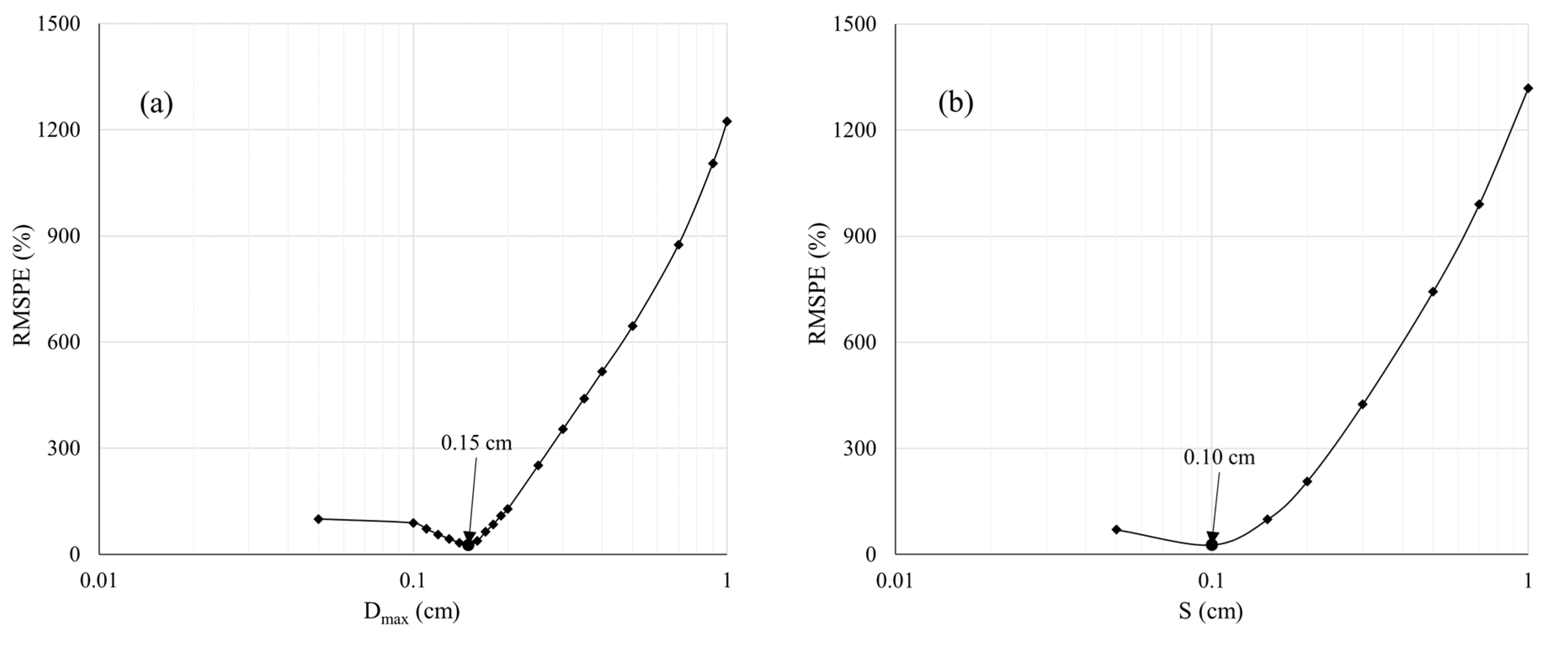
2.4. Reconstruction of 3D Plant Model

Raw LiDAR data were recorded in polar coordinates describing the angle (θ) from 0° to 180° and the distance (d) of each laser hit, which converted to Cartesian coordinates (x, y, z) with Python code (version 3.7, Python Software Foundation, Beaverton, OR, USA). Specifically, x-y planes were defined considering d from sensor centre as origin of coordinate system (Equations (1) and (2)). The displacement of LiDAR scanner in z direction was calculated from the constant forward speed (v) and time difference (Δt) between each vertical line of scan (Equations (3) and (4)).

$$x_{LiDAR}=d cos\theta$$

(1)

$$y_{LiDAR}=d sin\theta$$

(2)

$$z_{LiDAR}=z^{\prime }+∆z$$

(3)

$$∆z=v\times ∆t$$

(4)

where d is the distance between a laser point and the sensor, x_LiDAR and y_LiDAR signify the position of laser point in x and y axes, z_LiDAR is the LiDAR position along the linear conveyor axis, z’ is the previous position of LiDAR sensor, v is the forward speed of LiDAR sensor (0.01 ms⁻¹), and ∆z is the displacement of the LiDAR sensor during time ∆t (s).

A distance filter was applied to segment laser points above 2 m distance and discard points generated from background objects. In the pre-processing step, a statistical outlier removal (SOR) filter was applied based on the maximum distance calculated by the sum of mean distance and standard deviation of each point measured to its six neighboring points to determine whether it is an outlier [41]. Subsequently, the point clouds from both sides of strawberry plant were roughly aligned using open-source CloudCompare^® (version 2.10) software [42]. Fine registration was done by minimizing corresponding points’ distances according to the iterative closest point algorithm [43], resulting in a complete point cloud of each potted strawberry plant.

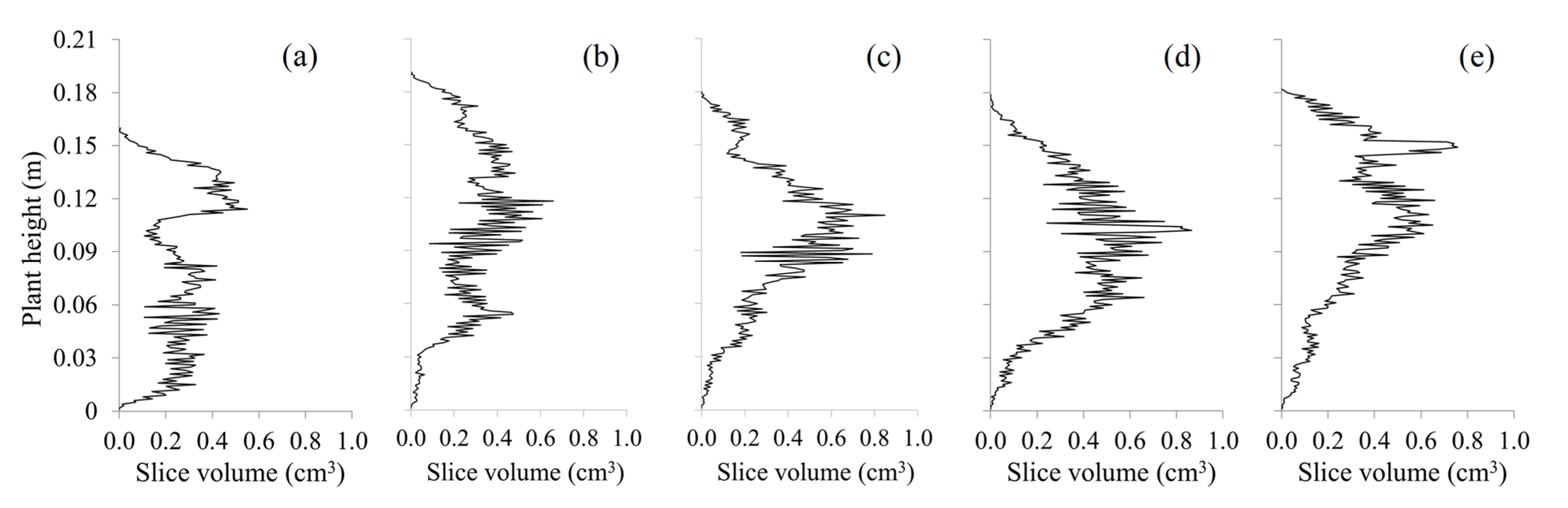
2.5. Estimation of Plant Parameters

The difference between maximum and minimum point of entire point cloud in the z axis including the growing container was exploited to estimate the plant height. Subsequently, the height of the container was subtracted manually.

The number of canopy points was plotted in the x and y axis. A line connected the points on the boundaries, creating a polygon. Subsequently, the concave hull algorithm was applied for estimating the projected canopy area of each plant [44].

Canopy volume was calculated by segmenting the canopy point cloud in horizontal slices of equal height (S). Each slice of varying height (0.05–10 cm) was projected in the x and y plane, while the Delaunay approach was performed for triangulation to create a network of triangles having no points inside circumscribing circles. The line connecting points was considered as an edge. The network of edges of the triangles was analyzed to detect holes and concavities. To extract holes or voids, a maximum point to point distance (D_max) was set based on minimizing the root mean square percentage error (RMSPE) for volume estimation. Edges greater than D_max were removed from the network. In the next step, the bounding polygon using the remaining edges was created. The edges present in the triangulated network were analysed individually. Only those edges that belong to a single triangle were selected [45], because only outer triangles can have edges not belonging to more than one triangle. After connecting the selected edges, one or more polygons were created. The area of the bounding polygon was recorded for each slice and multiplied by its height [46]. The sum provided the volume of canopy (Equation (5)) as one value (Figure 2).

$$V_{plant}={{\displaystyle \sum }}_{k=1}^n\left(A_k\times S\right)$$

(5)

where V_plant is total volume of strawberry canopy, k is number of slices, A_k is area of the k-th slice, and S is the height of the slice.

The performance of this slicing and summing slice volume estimation approach was compared with two widely-used volume estimation approaches: 3D convex hull [28,29] and voxel-grid [29,30], with a grid size of 1 cm. The accuracy of these three approaches was evaluated in terms of mean bias error (MBE), root mean square error (RMSE), RMSPE, and coefficient of determination (R²) between reference and estimated strawberry canopy volumes. Computational time was recorded and compared.

Applying the most accurate method, the volume of each slice was plotted against the canopy height to obtain the canopy volume profiles during plant growth. Strawberry plant growth rate was calculated from the changes in plant volume during the monitoring period (14 to 77 DAP) [47].

3. Results

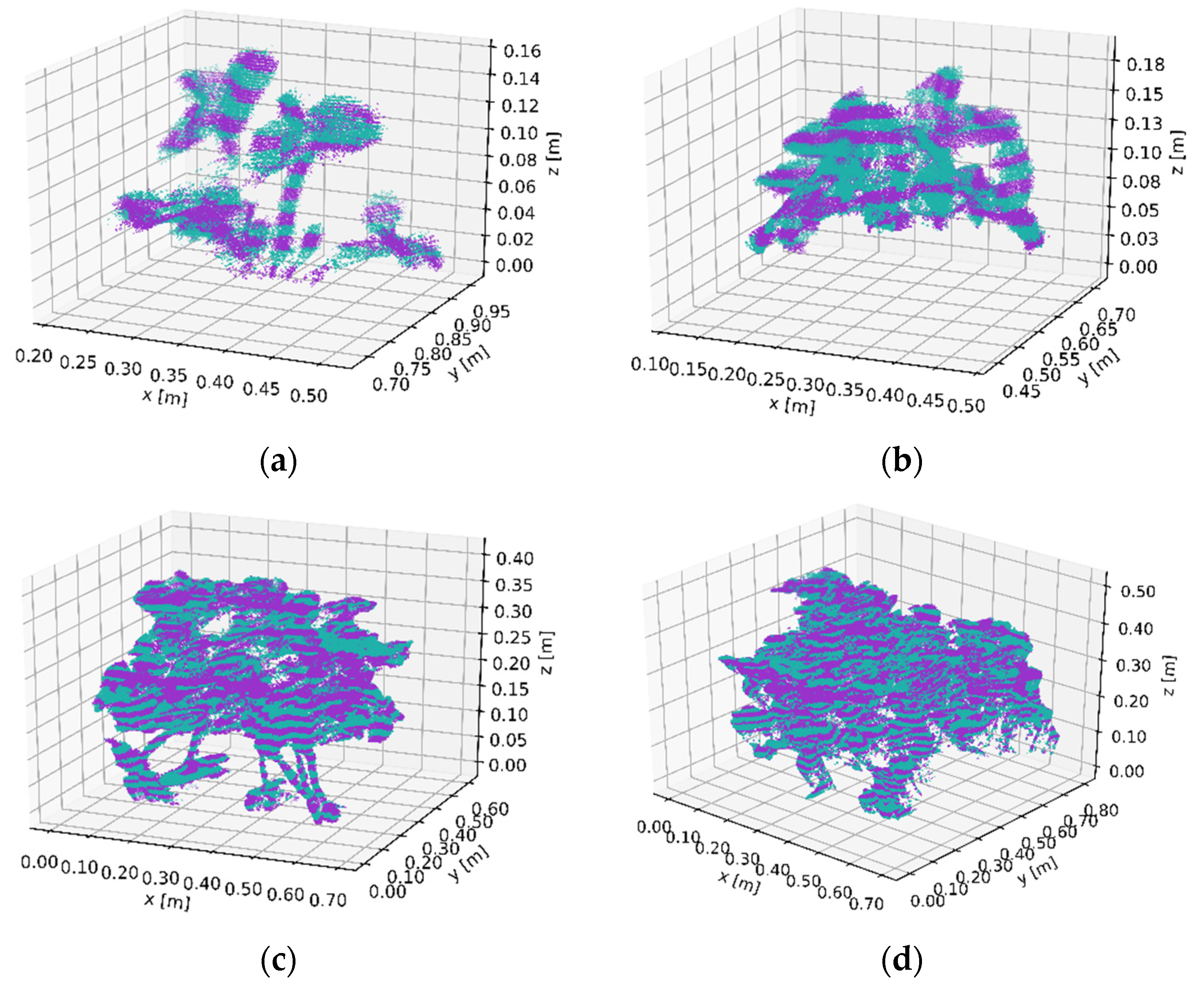
3.1. Canopy Volume Extraction Capturing Four Size Classes

Reconstructed 3D point clouds were obtained from outdoor measurement of four size classes of strawberry plants (Figure 2). Strawberry plants showed no consistent growth direction, while the shape varied over the plant developmental stages. In the juvenile stage, strawberry canopy was less dense (average 60,660 points per plant) compared with the matured stage (average 451,817 points per plant). In the juvenile stage, gaps and empty spaces were observed underneath the leaves, while the stem and petioles were still visible in the point clouds (Figure 2a,b). In the matured stage, stem and petioles disappeared from the 3D point cloud owing to a dense canopy with an enhanced number of leaves, but gaps and concavities were still present between the leaves (Figure 2c,d). The results obtained with established 3D point cloud analysis are consistent with earlier studies (

Table 1. Descriptive statistics of estimated strawberry canopy volume using three approaches (slicing and summing slice volume, voxel-grid, and 3D convex hull); errors are provided in terms of mean bias error (MBE), root mean square error (RMSE), root mean square percent error (RMSPE), coefficient of determination (R²) between estimated and reference volume (n = 12), and average computational time per plant.

Approach	Min (cm3)	Max (cm3)	SD (cm3)	Mean (cm3)	MBE (cm3)	RMSE (cm3)	RMSPE (%)	R2	Computational Time (s/plant)
Slicing and summing slices	43.9	97.2	13.7	71.0	−10.1	18.8	20.4	0.79	35.70
Voxel-grid	1692.0	2451.0	212.7	2134.3	2053.3	2062.3	2929.7	0.62	2534.00
3D convex hull	6064.2	17,341.9	2889.7	10,563.2	10,482.1	10,868.6	1,086,864	0.41	0.85

).

The approach of slicing and summing slice for volume estimation was tested on the strawberry point cloud slice considering the combination of two parameters—maximum point to point distance (D_max) and slice height (S). D_max has a key role in the proposed volume extraction approach to estimate an accurate canopy volume. The effect of D_max on area estimation is exemplarily visualized on point cloud slices of equal height considering three D_max values (0.15 cm, 1.0 cm, and 10.0 cm) in Figure 3. After removal of the boundary lines larger than D_max, the outer lines were applied to calculate the area of the polygon. Considering all size class cases, using D_max of 0.15 cm resulted in the lowest boundary and, therefore, area. The use of 10.0 cm D_max enhanced the estimated areas, whereas 0.15 cm was visually appropriate for removing gaps and voids, but not working on randomly appearing points.

The slicing and summing slice volume estimation approaches with D_max values ranging from 0.05 cm to 10.0 cm were applied on the point clouds of all size classes of strawberry plants, while S was still kept constant (0.1 cm) to demonstrate the effect of D_max (Figure 4). An overestimation became apparent in the estimated canopy volume of all size classes owing to the gradual increase of D_max. For D_max = 10.0 cm, the boundary line connected all the outer points, including the inner spaces and gaps of the slice, resulting in average canopy volumes of 2074 cm³, 3369 cm³, 50,768 cm³, and 105,360 cm³ for juvenile-1, juvenile-2, mature-1, and mature-2 size classes, respectively. With the smallest D_max (0.05 cm), the lowest areas for each horizontal slices were obtained as 0.023 cm³, 0.025 cm³, 0.046 cm³, and 0.133 cm³ considering average canopy volumes for juvenile-1, juvenile-2, mature-1, and mature-2 size classes, respectively. These volume results were certainly an underestimation of the actual volume, pointing to the necessary optimisation of D_max and S before application of the proposed volume approach.

To determine the optimum value of D_max and S, reference plant (n = 12) volume data obtained by water displacement technique were used. The proposed volume estimation technique was applied for all reference strawberry plant point clouds using a combination of D_max ranging from 0.05 cm to 1.0 cm and S ranging from 0.05 to 1.0 cm applied iteratively. Root mean squared percent error (RMSPE) between reference volume and volume obtained using the proposed approach showed RMSPE starting from 99.93% at 0.05 cm of D_max and gradually decreasing to 26.93% at 0.15 cm. However, RMSPE again increased with a higher D_max. D_max of 1 cm produced the highest RMSPE of 1318%. Similarly, the RMSPE for varying S from 0.05 to 1.0 cm, with D_max = 0.15 cm, is shown in Figure 5b. Minimal RMSPE values were found for S ≤ 0.1 cm, whereas enhanced S resulted in higher measuring uncertainty (Figure 5b). The computational time increased with enhanced D_max and reduced S (Figure 5c,d).

3.2. Comparative Analysis of Different Canopy Volume Estimation Approaches

The estimation of canopy volume of 12 reference strawberry plants was carried out using three approaches of 3D convex hull and voxel-grid methods along with the slicing and summing slice volume estimation approach. The comparison with manual measurement, which was done by the water displacement technique, confirms the feasibility of the proposed volume estimation approach with optimum parameters (D_max = 0.15 cm and S = 0.1 cm), as shown in Table 1. Voxel-grid returned slightly enhanced R² (0.62) compared with the 3D convex hull approach (R² = 0.41), because the voxel-grid approach was able to remove the gaps and holes within the canopy. However, estimation using the voxel-grid approach depends on the voxel-grid size and the approach requires a high computational time. The 3D convex hull approach does not require any optimization of parameters and was the fastest (0.85 s/plant) among these three approaches. However, it could not eliminate any gaps or holes within the point cloud, resulting in very high overestimation.

3.3. Summary Statistics and Correlations of Reference Plant Variables for Four Size Classes

The number of points per plant, canopy height, ground projected canopy area, and manually measured data (

Table 2. Descriptive statistics of LiDAR-estimated parameters (points per plant (PPP), height (h), and ground projected canopy area (canopy area)) and manually measured variables (fresh mass (FM), dry mass (DM), and leaf area (LA)) of strawberry canopies capturing four size classes (n = 15).

Descriptive Statistics	LiDAR Estimated Variables			Manually Measured Variables
	PPP	h (cm)	Canopy Area (cm2)	FM (g)	DM (g)	LA (cm2)
Min	34,459	8.73	311.59	11.15	3.86	409.92
Max	658,840	52.06	4555.31	382.09	131.92	19,336.00
Mean	243,200	27.38	1905.97	127.84	44.53	6522.55
Median	84,333	17.24	768.62	37.79	11.97	1369.32
Standard deviation	226,807	15.54	1659.92	130.66	45.40	7223.58
Skewness	0.80	0.39	0.48	0.91	0.80	0.87
Kurtosis	−0.82	−1.64	−1.54	−0.55	−0.78	−0.72

) appeared normally distributed. All parameters increased with enhanced plant size.

Fresh mass, dry mass, and leaf area of plants measured in the laboratory appeared to be correlated with LiDAR-estimated variables (

Table 3. Performance of derived model from dry mass, fresh mass, and leaf area of strawberry plants of four size classes (n = 15) with their LiDAR-estimated plant variables in terms of mean bias error (MBE), root mean square error (RMSE), root mean square percent error (RMSPE), and coefficient of determination (R²).

Model	LiDAR-Estimated Variables	MBE	RMSE	RMSPE (%)	R2
Fresh mass (g)	No. of points per plant	−0.0006	3.37	5.44	0.99
	Volume (cm3)	−0.0174	10.56	37.38	0.91
	Height (cm)	0.0073	8.67	30.72	0.93
	Projected canopy area (cm2)	0.0020	7.21	11.97	0.95
Dry mass (g)	No. of points per plant	−0.0003	1.00	4.45	0.99
	Volume (cm3)	−0.0010	3.36	37.09	0.92
	Height (cm)	0.0011	2.50	29.91	0.95
	Projected canopy area (cm2)	0.0002	2.09	10.87	0.97
Leaf area (cm²)	No. of points per plant	0.0010	258.03	12.84	0.98
	Volume (cm3)	35.1019	604.49	64.78	0.90
	Height (cm)	−1.3308	509.56	50.61	0.93
	Projected canopy area (cm2)	0.4246	370.43	22.66	0.96

). The number of points per plant 3D point cloud showed the highest coefficient of determination (R²) of 0.99, 0.99, and 0.98 with FM, DM, and leaf area, respectively, followed by other LiDAR-derived variables. However, the leaf area estimation appears to have high measuring uncertainty owing to occlusions in the dense canopies of mature plants.

3.4. Temporal Monitoring of Strawberry Canopy

3.4.1. Estimation of Leaf Area with LiDAR-Derived Canopy Variables of Juvenile Plants

Average size of leaf area found for ‘Honeoye’ was 87.69, 61.49, 93.13, 95.48, and 98.45 cm² at 14, 28, 50, 63, and 77 DAP, respectively. Similarly, for ‘M. Centenary’, the average sizes of leaves recorded were 68.32, 92.31, 88.97, 94.24, and 98.93 cm² at 14, 28, 42, 56, and 70 DAP, respectively. The leaf size increased during plant development. Older leaves that accumulated high biomass and leaf area were expanded, resulting in enhanced leaf density in mature leaves compared with young leaves. To obtain the relationships between manually measured leaf area of strawberry plants and LiDAR-derived variables, linear regression analysis was performed. The leaf area was highly correlated to the number of points in 3D point clouds (R² = 0.78). Furthermore, LiDAR-estimated canopy volume revealed a high correlation with the leaf area. However, a reduced correlation was observed between the LiDAR-estimated plant height and ground projected canopy area with leaf area in juvenile plants (R² = 0.20 and 0.25). However, these relationships were more pronounced when all size classes were considered (R² = 0.93 and 0.96), outweighing the effect of straight upright growth of young leaves in juvenile plants and measuring uncertainty due to dense canopies.

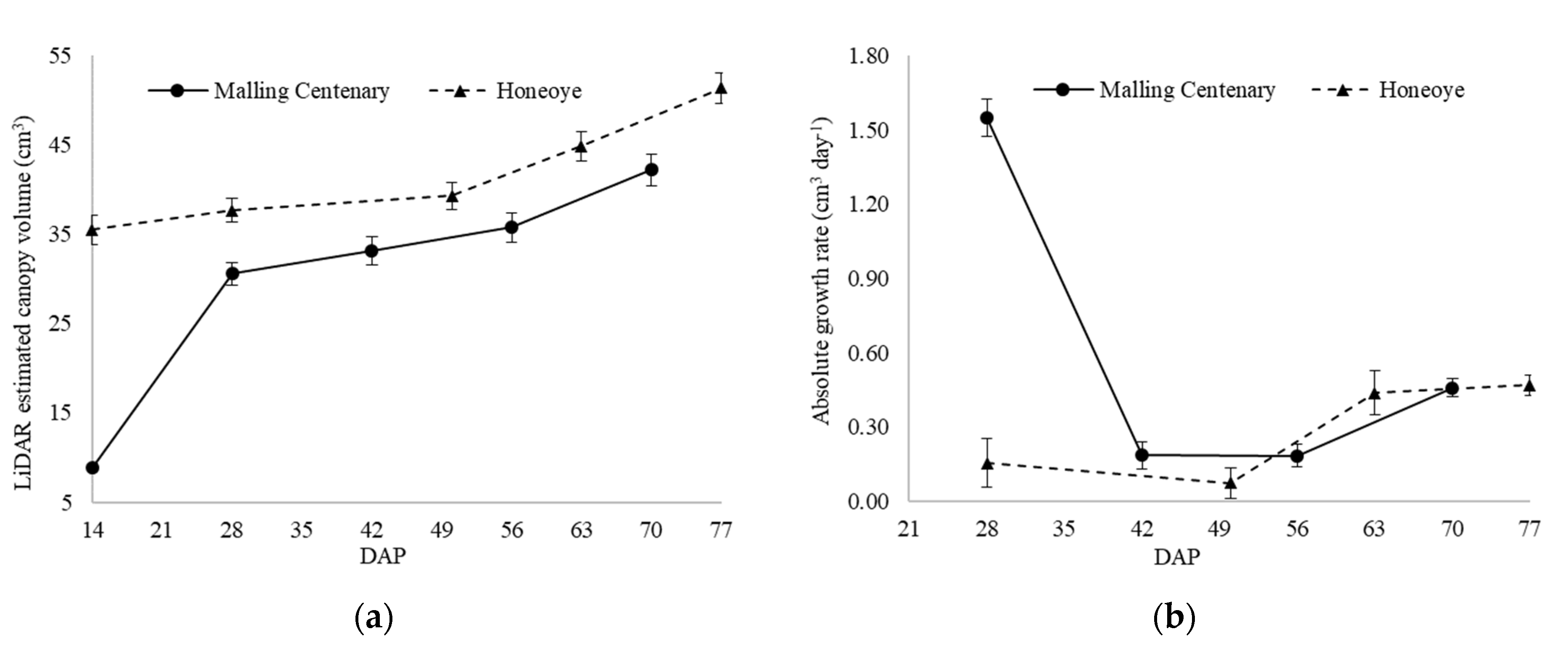
3.4.2. Canopy Volume

The juvenile development of two strawberry cultivars was measured in situ with LiDAR scanner in outdoor conditions throughout the growing season. The canopy volume was estimated from 3D LiDAR point cloud data using the proposed volume estimation method with D_max 0.15 cm and S = 0.10 cm according to the findings on reference plant volume obtained by the water displacement method. Both cultivars showed a gradual change in volume during the measurement period (Figure 6a). However, cultivar ‘Malling Centenary’ showed a rapid increase from 14 to 28 DAP compared with cultivar ‘Honeoye’. In the following observations, a similar progressive increase in canopy volume was found for both cultivars. The first LiDAR scan was performed at 14 DAP, when leaves (n = 5–7) were immature and standing straight upwards. Subsequently, more leaves grew and young leaves were expanded, and the old leaves were laid down, losing their upright habitus owing to increase in mass and loss of turgor. Consistently, the shape of plants changed during the observation period. The average volume was increased from 35.5 cm³ to 51.36 cm³ for ‘Honeoye’ cultivar, whereas for the ‘Malling Centenary’, the average volume was increased from 8.92 cm³ to 42.18 cm³.

Absolute growth rates of the strawberry plants of both cultivars were determined from the change in plant volume (Figure 6b). It was found that, at 28 DAP, the absolute growth rate was higher for the ‘Malling Centenary’ cultivar (1.55 cm³ day⁻¹) compared with ‘Honeoye’ (0.15 cm³ day⁻¹). However, the growth rate of ‘Malling Centenary’ declined sharply in next 14 days. Conversely, ‘Honeoye’ cultivar showed a gradual increase in the absolute growth rate and displayed 0.47 cm³ day⁻¹ at DAP.

Time series of change in vertical volume profile were obtained when plotting the histogram of points per plant. Data are shown for a typical sample plant from 14 to 77 DAP (Figure 7). Optimum D_max (0.15 cm) and S (0.10 cm) found in this study (Figure 5) provided the most realistic LiDAR-estimated volume. From the time series of vertical volume profiles, it can be observed that the plants showed changes in volume and shape. At 14 DAP (Figure 7a), when the plants showed 3–5 leaves, the existing leaves had long petiole standing upwards, which was accountable for almost similar canopy height. At 28 DAP, new leaves were developing and the shape of profile changed with the upper part producing higher volumes. Subsequently, leaf area and total canopy volume increased until 77 DAP (Figure 7e).

4. Discussion

In this study, a canopy growth estimation by means of 3D LiDAR point cloud analysis was proposed and evaluated on four different size classes of strawberry canopy ranging from young to mature. Vegetative growth of juvenile strawberry plants was assessed over the season in terms of adapted canopy volume estimated by LiDAR laser scanner introducing vertical canopy volume profiling in strawberry plants.

Yamamoto and co-workers [20] used a depth camera system placed in a stationary position while strawberry plants were placed on a movable planting bench underneath. In the present experiment, a 2D LiDAR laser scanner was mounted on a linear, electric conveyor to scan each individual strawberry plant with growing container from two sides in the fruit production environment. Because of the electric engine, LiDAR movement during scanning strawberry plants was reduced considering perturbation due to 3D rotation (roll, pitch, and yaw). However, measurements were carried out in outdoor conditions. While the light is supposed to be a marginal influencing factor in LiDAR measurements, the wind has an impact on the data, because strawberry plants have no stiff woody structure. Therefore, wind can cause considerable height reduction and shape deformation visible in the point cloud. To overcome this challenge, extreme weather conditions were avoided, but an influence can still be assumed.

Slicing the point cloud and estimation of individual slice volume method proposed in this study was applied for strawberry canopy volume estimation in different plant sizes. Xu et al. [33] proposed a tree crown volume estimation approach by slicing the point cloud, but applying a different slice volume estimation method. As the strawberry plants show an irregular shape and structure, the present volume estimation approach targeted the removal of gaps. An effective approach was shown by Yan et al. [35] for estimation of point cloud slice to calculate the canopy volume of individual trees and found the smallest volume compared with other existing canopy volume estimation methods. In this study, two parameters were introduced to improve the volume estimation accuracy: slicing and adapted D_max and S, which were calibrated by measuring the canopy volume by means of the water displacement technique. Different S (0.05–10 cm) were tested along with varying D_max values ranging from 0.05 to 10 cm. The lowest RMSPE was found for 0.1 cm and 0.15 cm of S and D_max, respectively. The resulting RMSPE was still rather high with >20%, but comparatively smaller than the RMSPE found for different combinations of S and D_max. The computational complexity was observed in terms of average time required per plant. The computational time varied with slice height as it determined the number of iterations. The optimum combination of parameters (0.1 cm S and 0.15 cm D_max) resulted in 35.70 s, whereas computation time decreased gradually to 13.12 s (S = 0.5 cm and D_max = 0.15 cm) and 10.42 s (S = 1.0 cm and D_max = 0.15 cm). The optimum combination of parameters yielded a low RMSPE (26.93%). This sets the benchmark, because so far, hardly any studies exist using the actual volume of the canopy instead of comparing methods without the actual ground truth.

Subsequently, after finding the optimum parameters of the proposed volume estimation approach, two other existing tree canopy volume estimation approaches (3D convex hull and voxel-grid) were compared. Effective removing of gaps and holes within the canopy was important, and reducing the computational time was in consideration. A 3D convex hull was widely used volume estimation from 3D point cloud data owing to its faster computational time. However, it could not meet the acceptable accuracy for the irregular-shaped 3D point cloud such as tree canopy when compared with accurate reference volume as shown in this study. Because its bounding geometrical approach included all the holes and cavities presented in the point cloud [34], the voxel-grid approach resulted in higher accuracy than the 3D convex hull approach for the strawberry point cloud. However, voxelization of 3D point cloud data required a high computational time and power, which mostly depended on the size of the voxel grid. The smaller voxel size is able to estimate volumes with enhanced accuracy, but it also has a high computational time cost. Therefore, optimization of voxel size can be considered as a limitation of this approach [48]. Both of these approaches were applied previously for estimation of tree crown volume in orchard or forestry where reference volume was determined by different geometrical shape approaches. In this study, methods were compared to precise reference volume determined by water displacement technique. In comparison, slicing and summing slice volume estimation approach was found more accurate and required less computational time than voxel-grid in this study.

Hosoi et al. [30] demonstrated the method for analyzing the vertical distribution of volume for individual trees estimated by voxel-based volume estimation. In the present study, time series of LiDAR 3D point cloud analysis revealed the growth patterns of juvenile strawberry plants based on total canopy volume of the two strawberry cultivars. Furthermore, the time series of canopy volume profiles additionally revealed the pattern of change in volume distribution along the vertical canopy axis (Figure 7). At first measurement at 14 DAP of plantation, an average of 5–7 leaves was found, and most of them were standing upward. Both cultivars have shown similar growth patterns considering the straight upright leaves and petioles after planting and subsequently more mature leaves with smaller and shorter petioles. More physiological explanation was provided by Takahashi et al. [19]. The authors applied an RGB-depth camera, which is affected by varying lighting conditions and, therefore, is difficult to use in a production environment. However, the effect of temperature and amount of light received by the leaves on the strawberry plant height was shown. With the present benchmark of volume estimation, a methodology is available for further physiological analysis and support of variable rate plant protection considering the volume profile of the canopies (Figure 7).

LiDAR point cloud derived plant geometrical parameters were correlated to other destructively measured variables. Strong linear relationships were observed for the number of points per plant with dry mass (R² = 0.99) and fresh mass (R² = 0.99) of plants. LiDAR derived plant volume also demonstrated good linear relationships for dry mass (R² = 0.92) and fresh mass (R² = 0.90). Walter el al. [49] found high correlations between above ground biomass and LiDAR estimated volume up to r = 0.86 for wheat. Greaves et al. [50] also revealed a strong correlation (R² = 0.92) between harvested biomass and LiDAR-estimated volume for arctic shrubs using terrestrial laser scanning in a close range (2 m). However, plant height and ground projected canopy area exhibited weaker linear relationships with dry mass and fresh mass of plants. Guan et al. [21] tested the linear relationship of similar parameters, although he used an RGB image to reconstruct point cloud using a structure from motion algorithm. With this approach, R² = 0.77 was found for canopy volume and dry mass. For LA observation, Guan et al. [21] found R² = 0.76 between canopy volume and LA, whereas the current results showed R² = 0.97 when all size classes of strawberry plants were considered. As a result, LiDAR point cloud derived strawberry plant parameters could be utilized to model the strawberry plant growth. The introduction of the method in physiological studies or applications in variable rate management should be investigated in future studies.

5. Conclusions

In this study, the 2D LiDAR laser scanner was mounted on a mobile linear conveyor to scan commercial strawberry plants. This type of linear conveyor mounted 2D LiDAR laser scanner can be further applied in greenhouse or greenhouse crop monitoring, providing 3D dataset of the plants.

A volume estimation technique was proposed based on slicing and summing slice volume from 3D strawberry point cloud. The approach enabled the removal of holes and gaps, resulting in R² = 0.80 with a low computational time. Moreover, this approach was capable of extracting volumes of different horizontal layers of canopy, which can generate the vertical canopy volume profile of strawberry plant. Analysis of time series of 3D point cloud data revealed the typical growing pattern of strawberry plants in the vertical canopy profiles.

The relationship between various LiDAR point cloud derived parameters with destructively measured biomass and geometry was confirmed in this study. In conclusion, LiDAR laser scanners mounted on near-ground linear conveyor are a feasible tool for monitoring strawberry plant growth.

References

1. An, X.; Li, Z.; Zude-Sasse, M.; Tchuenbou-Magaia, F.; Yang, Y. Characterization of textural failure mechanics of strawberry fruit. J. Food Eng. 2020, 282, 110016. [Google Scholar] [CrossRef]
2. Weng, S.Z.; Yu, S.; Dong, R.L.; Pan, F.F.; Liang, D. Nondestructive detection of storage time of strawberries using visible/near-infrared hyperspectral imaging. Int. J. Food Prop. 2020, 23, 269–281. [Google Scholar] [CrossRef] [Green Version]
3. Darnell, R.L.; Cantliffe, D.J.; Kirschbaum, D.S.; Chandler, C.K. The Physiology of Flowering in Strawberry. Hortic. Rev. 2002, 28, 325–349. [Google Scholar] [CrossRef]
4. Zude-Sasse, M.; Fountas, S.; Gemtos, T.; Abu-Khalaf, N. Applications of precision agriculture in horticultural crops. Eur. J. Hortic. Sci. 2016, 81, 78–90. [Google Scholar] [CrossRef]
5. Johnson, R.S.; Lakso, A.N. Approaches to Modeling Light Interception in Orchards. HortScience 1991, 26, 1002–1004. [Google Scholar] [CrossRef] [Green Version]
6. Weiss, M.; Jacob, F.; Duveiller, G. Remote sensing for agricultural applications: A meta-review. Remote Sens. Environ. 2020, 236, 111402. [Google Scholar] [CrossRef]
7. Khanal, S.; Kc, K.; Fulton, J.; Shearer, S.; Ozkan, E. Remote Sensing in Agriculture—Accomplishments, Limitations, and Opportunities. Remote Sens. 2020, 12, 3783. [Google Scholar] [CrossRef]
8. Fahlgren, N.; A Gehan, M.; Baxter, I. Lights, camera, action: High-throughput plant phenotyping is ready for a close-up. Curr. Opin. Plant Biol. 2015, 24, 93–99. [Google Scholar] [CrossRef] [Green Version]
9. Klodt, M.; Herzog, K.; Töpfer, R.; Cremers, D. Field phenotyping of grapevine growth using dense stereo reconstruction. BMC Bioinform. 2015, 16, 143. [Google Scholar] [CrossRef] [PubMed] [Green Version]
10. Klose, R.; Penlington, J.; Ruckelshausen, A. Usability study of 3d time-of-flight cameras for automatic plant phenotyping. Bornimer Agrartech. Ber. 2009, 69, 12. [Google Scholar]
11. Wang, Z.; Walsh, K.B.; Verma, B. On-Tree Mango Fruit Size Estimation Using RGB-D Images. Sensors 2017, 17, 2738. [Google Scholar] [CrossRef] [Green Version]
12. Chéné, Y.; Rousseau, D.; Lucidarme, P.; Bertheloot, J.; Caffier, V.; Morel, P.; Belin, É.; Chapeau-Blondeau, F. On the use of depth camera for 3d phenotyping of entire plants. Comput. Electron. Agric. 2012, 82, 122–127. [Google Scholar] [CrossRef]
13. Polo, J.R.R.; Sanz, R.; Llorens, J.; Arnó, J.; Escolà, A.; Ribes-Dasi, M.; Masip, J.; Camp, F.; Gràcia, F.; Solanelles, F.; et al. A tractor-mounted scanning LIDAR for the non-destructive measurement of vegetative volume and surface area of tree-row plantations: A comparison with conventional destructive measurements. Biosyst. Eng. 2009, 102, 128–134. [Google Scholar] [CrossRef] [Green Version]
14. Tsoulias, N.; Paraforos, D.S.; Fountas, S.; Zude-Sasse, M. Estimating Canopy Parameters Based on the Stem Position in Apple Trees Using a 2D LiDAR. Agronomy 2019, 9, 740. [Google Scholar] [CrossRef] [Green Version]
15. Soudarissanane, S.; Lindenbergh, R.; Menenti, M.; Teunissen, P. Scanning geometry: Influencing factor on the quality of terrestrial laser scanning points. ISPRS J. Photogramm. Remote Sens. 2011, 66, 389–399. [Google Scholar] [CrossRef]
16. Herrero-Huerta, M.; Bucksch, A.; Puttonen, E.; Rainey, K.M. Canopy Roughness: A New Phenotypic Trait to Estimate Aboveground Biomass from Unmanned Aerial System. Plant Phenomics 2020, 2020, 1–10. [Google Scholar] [CrossRef]
17. Tsoulias, N.; Paraforos, D.; Xanthopoulos, G.; Zude-Sasse, M. Apple Shape Detection Based on Geometric and Radiometric Features Using a LiDAR Laser Scanner. Remote Sens. 2020, 12, 2481. [Google Scholar] [CrossRef]
18. Zhou, H.; Zhang, J.; Ge, L.; Yu, X.; Wang, Y.; Zhang, C. Research on volume prediction of single tree canopy based on three-dimensional (3D) LiDAR and clustering segmentation. Int. J. Remote Sens. 2021, 42, 738–755. [Google Scholar] [CrossRef]
19. Takahashi, M.; Takayama, S.; Umeda, H.; Yoshida, C.; Koike, O.; Iwasaki, Y.; Sugeno, W. Quantification of Strawberry Plant Growth and Amount of Light Received Using a Depth Sensor. Environ. Control Biol. 2020, 58, 31–36. [Google Scholar] [CrossRef] [Green Version]
20. Yamamoto, S.; Hayashi, S.; Tsubota, S. Growth Measurement of a Community of Strawberries Using Three-Dimensional Sensor. Environ. Control Biol. 2015, 53, 49–53. [Google Scholar] [CrossRef]
21. Guan, Z.; Abd-Elrahman, A.; Fan, Z.; Whitaker, V.M.; Wilkinson, B. Modeling strawberry biomass and leaf area using object-based analysis of high-resolution images. ISPRS J. Photogramm. Remote Sens. 2020, 163, 171–186. [Google Scholar] [CrossRef]
22. Han, K.-S.; Kim, S.-C.; Lee, Y.-B.; Kim, S.-C.; Im, D.-H.; Choi, H.-K.; Hwang, H. Strawberry Harvesting Robot for Bench-type Cultivation. J. Biosyst. Eng. 2012, 37, 65–74. [Google Scholar] [CrossRef] [Green Version]
23. Ge, Y.; Xiong, Y.; From, P.J. Symmetry-based 3D shape completion for fruit localisation for harvesting robots. Biosyst. Eng. 2020, 197, 188–202. [Google Scholar] [CrossRef]
24. Zhou, C.; Hu, J.; Xu, Z.; Yue, J.; Ye, H.; Yang, G. A Novel Greenhouse-Based System for the Detection and Plumpness Assessment of Strawberry Using an Improved Deep Learning Technique. Front. Plant Sci. 2020, 11, 559. [Google Scholar] [CrossRef]
25. He, J.Q.; Harrison, R.J.; Li, B. A novel 3D imaging system for strawberry phenotyping. Plant Methods 2017, 13, 1–8. [Google Scholar] [CrossRef]
26. Li, B.; Cockerton, H.M.; Johnson, A.W.; Karlström, A.; Stavridou, E.; Deakin, G.; Harrison, R.J. Defining strawberry shape uniformity using 3d imaging and genetic mapping. Hortic. Res. 2020, 7, 1–13. [Google Scholar] [CrossRef]
27. Directive, C. Council directive 91/414/eec of 15 july 1991 concerning the placing of plant protection products on the market. Off. J. Eur. Communities L 1991, 230, 1–32. [Google Scholar]
28. Cheein, F.A.A.; Guivant, J.; Sanz, R.; Escolà, A.; Yandún, F.; Torres-Torriti, M.; Rosell-Polo, J.R. Real-time approaches for characterization of fully and partially scanned canopies in groves. Comput. Electron. Agric. 2015, 118, 361–371. [Google Scholar] [CrossRef] [Green Version]
29. Colaço, A.F.; Trevisan, R.G.; Molin, J.P.; Rosell-Polo, J.R.; Escolà, A. A Method to Obtain Orange Crop Geometry Information Using a Mobile Terrestrial Laser Scanner and 3D Modeling. Remote Sens. 2017, 9, 763. [Google Scholar] [CrossRef] [Green Version]
30. Hosoi, F.; Nakai, Y.; Omasa, K. 3-D voxel-based solid modeling of a broad-leaved tree for accurate volume estimation using portable scanning lidar. ISPRS J. Photogramm. Remote Sens. 2013, 82, 41–48. [Google Scholar] [CrossRef]
31. Underwood, J.; Hung, C.; Whelan, B.; Sukkarieh, S. Mapping almond orchard canopy volume, flowers, fruit and yield using lidar and vision sensors. Comput. Electron. Agric. 2016, 130, 83–96. [Google Scholar] [CrossRef]
32. Putman, E.B.; Popescu, S.C. Automated Estimation of Standing Dead Tree Volume Using Voxelized Terrestrial Lidar Data. IEEE Trans. Geosci. Remote Sens. 2018, 56, 6484–6503. [Google Scholar] [CrossRef]
33. Xu, W.; Su, Z.; Feng, Z.; Xu, H.; Jiao, Y.; Yan, F. Comparison of conventional measurement and LiDAR-based measurement for crown structures. Comput. Electron. Agric. 2013, 98, 242–251. [Google Scholar] [CrossRef]
34. Lin, W.; Meng, Y.; Qiu, Z.; Zhang, S.; Wu, J. Measurement and calculation of crown projection area and crown volume of individual trees based on 3D laser-scanned point-cloud data. Int. J. Remote Sens. 2017, 38, 1083–1100. [Google Scholar] [CrossRef]
35. Yan, Z.; Liu, R.; Cheng, L.; Zhou, X.; Ruan, X.; Xiao, Y. A Concave Hull Methodology for Calculating the Crown Volume of Individual Trees Based on Vehicle-Borne LiDAR Data. Remote Sens. 2019, 11, 623. [Google Scholar] [CrossRef] [Green Version]
36. Escolà, A.; Martínez-Casasnovas, J.A.; Rufat, J.; Arnó, J.; Arbonés, A.; Sebé, F.; Pascual, M.; Gregorio, E.; Rosell-Polo, J.R. Mobile terrestrial laser scanner applications in precision fruticulture/horticulture and tools to extract information from canopy point clouds. Precis. Agric. 2017, 18, 111–132. [Google Scholar] [CrossRef] [Green Version]
37. Meier, U.; Graf, H.; Hack, H.; Hess, M.; Kennel, W.; Klose, R.; Mappes, D.; Seipp, D.; Stauss, R.; Streif, J. Phenological growth stages of pome fruit (Malus domestica borkh. and Pyrus Communis L.), stone fruit (Prunus species), Currants ribes species and strawberry (Fragaria × ananassa duch.). Nachr. Dtsch. Pflanzenschutzd. 1994, 46, 141–153. [Google Scholar]
38. Hobart, M.; Pflanz, M.; Weltzien, C.; Schirrmann, M. Growth Height Determination of Tree Walls for Precise Monitoring in Apple Fruit Production Using UAV Photogrammetry. Remote Sens. 2020, 12, 1656. [Google Scholar] [CrossRef]
39. Lawlor, D.W.; Boyle, F.A.; Keys, A.J.; Kendall, A.C.; Young, A.T. Nitrate Nutrition and Temperature Effects on Wheat: A Synthesis of Plant Growth and Nitrogen Uptake in Relation to Metabolic and Physiological Processes. J. Exp. Bot. 1988, 39, 329–343. [Google Scholar] [CrossRef]
40. Harrington, J.T.; Mexal, J.G.; Fisher, J.T. Volume displacement provides a quick and accurate way to quantify new root production. Seedling 1994, 121, 124. [Google Scholar]
41. Rusu, R.B.; Marton, Z.C.; Blodow, N.; Dolha, M.; Beetz, M. Towards 3D Point cloud based object maps for household environments. Robot. Auton. Syst. 2008, 56, 927–941. [Google Scholar] [CrossRef]
42. Girardeau-Montaut, D. Cloudcompare, v. 2.10. 2019. Available online: https://cloudcompare.org (accessed on 2 May 2020).
43. Besl, P.J.; McKay, N.D. Method for registration of 3-D shapes. Proceedings of Sensor Fusion IV: Control Paradigms and Data Structures, Boston, MA, USA, 14–15 November 1991; pp. 586–606. [Google Scholar]
44. Moreira, A.; Santos, M.Y. Concave Hull: A K-Nearest Neighbors Approach for the Computation of the Region Occupied by A Set of Points. In Proceedings of the GRAPP 2007 International Conference on Computer Graphics Theory and Applications, Barcelona, Spain, 8–11 March 1991; Volume 2, pp. 61–68. [Google Scholar]
45. Awrangjeb, M. Using point cloud data to identify, trace, and regularize the outlines of buildings. Int. J. Remote Sens. 2016, 37, 551–579. [Google Scholar] [CrossRef]
46. Saha, K.; Tsoulias, N.; Zude-Sasse, M. Estimation of leaf area of sweet cherry trees trained as spindle using ground based 2D mobile LiDAR system. Acta Hortic. 2021, 8, 429–436. [Google Scholar] [CrossRef]
47. Hunt, R. Plant Growth Curves. The Functional Approach to Plant Growth Analysis; Edward Arnold Ltd.: London, UK, 1982. [Google Scholar]
48. Lecigne, B.; Delagrange, S.; Messier, C. Exploring trees in three dimensions: VoxR, a novel voxel-based R package dedicated to analysing the complex arrangement of tree crowns. Ann. Bot. 2017, 121, 589–601. [Google Scholar] [CrossRef] [PubMed]
49. Walter, J.D.C.; Edwards, J.; McDonald, G.; Kuchel, H. Estimating Biomass and Canopy Height with LiDAR for Field Crop Breeding. Front. Plant Sci. 2019, 10, 1145. [Google Scholar] [CrossRef] [PubMed]
50. Greaves, H.E.; Vierling, L.A.; Eitel, J.U.H.; Boelman, N.T.; Magney, T.S.; Prager, C.M.; Griffin, K.L. Estimating aboveground biomass and leaf area of low-stature Arctic shrubs with terrestrial LiDAR. Remote Sens. Environ. 2015, 164, 26–35. [Google Scholar] [CrossRef]
Figure 1. (a) Photograph of the LiDAR laser scanning system (LMS511 pro, Sick AG, Düsseldorf, Germany) during strawberry plant measurement and (b) a schematic view of the LiDAR system mounted on a linear conveyor measuring strawberry 3D point cloud. θ is the angular step and d is the measured distance by the LiDAR laser scanner.
Horticulturae 08 00090 g001
Figure 2. Point cloud of different size classes of strawberry plants: (a) juvenile-1, (b) juvenile-2, (c) mature-1, and (d) mature-2. In these figures, 1 cm slice height is shown for visualization.
Horticulturae 08 00090 g002
Figure 3. Estimated areas from single point cloud slices with 0.1 cm height for different size classes of strawberry plants using different Dmax (0.15 cm, 1.0 cm, and 10.0 cm): (a) juvenile-1, (b) juvenile-2, (c) mature-1, and (d) mature-2.
Horticulturae 08 00090 g003
Figure 4. Changes in strawberry canopy volume due to an increase in Dmax from 0.05 cm to 10.0 cm when S is constant (0.1 cm) of different size classes of strawberry plant (n = 15). Logarithmic scale was used for data visualization purposes.
Horticulturae 08 00090 g004
Figure 5. Changes in root mean squared percentage error (RMSPE) between reference strawberry plant (n = 12) volume determined by water displacement technique and 3D point cloud estimated volume using slicing and summing slice volume approach considering varying Dmax for S = 0.1 cm (a) and varying S for Dmax = 0.15 cm (b). Computational time plotted for corresponding cases (c) and (d). For enhancing readability, the x-axis is shown on log scale in the first two figures.
Horticulturae 08 00090 g005aHorticulturae 08 00090 g005b
Figure 6. (a) Increase in strawberry canopy volume estimated from LiDAR point cloud and (b) absolute growth rate (cm3 day−1) of two strawberry cultivars in term of plant volume over time in days after planting (DAP).
Horticulturae 08 00090 g006
Figure 7. Vertical canopy volume profiles obtained using Dmax = 0.15 cm and slight height S = 0.1 cm considering a typical strawberry plant from time series LiDAR data acquired on 14, 28, 50, 63 and 77 days after planting (DAP) shown in (ae), respectively.
Horticulturae 08 00090 g007