Article

Development of Growth Estimation Algorithms for Hydroponic Bell Peppers Using Recurrent Neural Networks

1
Department of Smart Agriculture, Jeonju University, Jeonju 55069, Korea
2
Department of Agriculture, Forestry and Bioresources, Seoul National University, Seoul 08826, Korea
3
Research Institute of Agriculture and Life Sciences, Seoul National University, Seoul 08826, Korea
*
Author to whom correspondence should be addressed.
Horticulturae 2021, 7(9), 284; https://doi.org/10.3390/horticulturae7090284
Submission received: 19 July 2021 / Revised: 27 August 2021 / Accepted: 30 August 2021 / Published: 3 September 2021

Abstract

:
As smart farms are applied to agricultural fields, the use of big data is becoming important. In order to efficiently manage smart farms, relationships between crop growth and environmental conditions are required to be analyzed. From this perspective, various artificial intelligence algorithms can be used as useful tools to quantify this relationship. The objective of this study was to develop and validate an algorithm that can interpret the crop growth rate response to environmental factors based on a recurrent neural network (RNN), and to evaluate the algorithm accuracy compared to the process-based model (PBM). The algorithms were trained with data from three growth periods. The developed methods were used to measure the crop growth rate. The algorithm consisted of eight environmental variables days after transplanting and two crop growth characteristics as input variables producing weekly crop growth rates as output. The RNN-based crop growth rate estimation algorithm was validated using data collected from a commercial greenhouse. The CropGro-bell pepper model was applied to compare and evaluate the accuracy of the developed algorithm. The training accuracies varied from 0.75 to 0.81 in all growth periods. From the validation result, it was confirmed that the accuracy was reliable in the commercial greenhouse. The accuracy of the developed algorithm was higher than that of the PBM. The developed algorithm can contribute to crop growth estimation with a limited number of data.

1. Introduction

Smart farming is about applying new digital technologies such as remote sensing [1], cloud computing [2], and the Internet of Things (IoT) [3] to agricultural fields. These digital technologies contribute to large amounts of data at unprecedented rates [4,5]. Based on the increasing number of data, many studies trying to utilize big data were conducted [6]. For the efficient use of big data from the agricultural fields, it is necessary to quantitatively analyze the complex, diverse, and unpredictable relationship between crop growth and environmental factors [7]. Many studies have been conducted using process-based models (PBMs) to analyze the relationship [8]. PBM consists of many modules that express various crop physiological processes (e.g., photosynthesis, respiration, biomass assimilation, biomass distribution, and stress response). As PBM aims to include all biochemical functions, various modules are subjected to interlinked calculations for even a single variable and calibration of many indexes is required [9,10]. In addition, it is important to partition crop organ biomass to accurately simulate models because PBM estimates biomass production through the distribution to each organ [11,12]. In these respects, PBM has limitations directly utilizing big data that have been automatically accumulated.
An artificial neural network (ANN) provides a way of analyzing complex, non-linear, and multidimensional datasets from big data [13], and can abstract quantitative relationships from raw data [14]. ANN has been widely used in agricultural studies to analyze the biochemical and physiological characteristics for various crops [15,16,17].
Among ANN algorithms, the recurrent neural network (RNN) is the most promising for analyzing chronological data and displays better accuracy than previous algorithms [18,19]. RNNs have the advantage of inputting big data over long time periods and the length of output values is also theoretically unlimited [20]. With these advantages, RNNs have been adapted for agricultural purposes and showed higher accuracies than other algorithms [21,22,23]. The previous studies showed the adaptability of RNNs for environmental data but the RNNs were not trained to directly relate the environment and crop growth. As crop growth responses to the environment are determined by changes over the time of environmental factors, RNN would be appropriate to estimate the crop growth response for cumulative environmental changes. This study aims to develop an RNN algorithm to assess crop growth in response to various environmental factors in hydroponically grown bell peppers. In addition, the developed algorithm was validated by comparing it with an existing PBM.

2. Materials and Methods

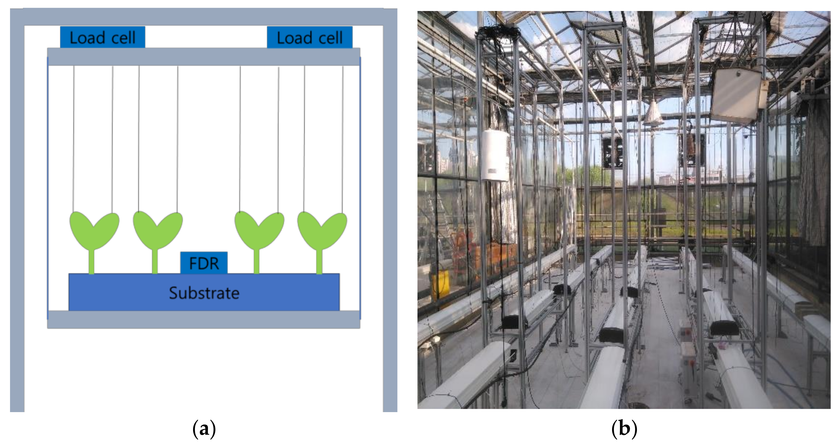
2.1. Crop Growth Conditions for Algorithm Training

The data collecting for algorithm training were conducted in a Venlo-type greenhouse on the experimental farm of Seoul National University, Suwon, Korea (latitude, 37.3° N; longitude, 127.0° E) during 1 February to 1 June 2018 (growth period 1) and 1 December 2018 to 1 April 2019 (growth period 2), and in a Venlo-type greenhouse on the experimental farm of Nong Woo Bio Ansung, Korea (latitude, 37.0° N; longitude, 127.0° E) during 1 September to 1 December 2018 (growth period 3). The data collecting for validation is described in Section 2.4. The vents on the roof and sidewall were automatically opened when the temperature was higher than 26 °C during the day. Bell pepper seedlings (Capsicum annuum L. ‘Sirocco’) 40 days after sowing on rockwool cubes (Grodan delta, Grodan, Roermond, The Netherlands) in a seedling chamber were used. After two weeks of acclimatization to the irrigation system at an electrical conductivity (EC) of 2.0 dS/m, the seedlings with 5–6 nodes were transplanted into 0.9 ∗ 0.15 ∗ 0.07 m (L ∗ W ∗ H) rockwool slabs (Grotop GT Master Dry, Grodan, Roermond, The Netherlands) and placed on gutters with a plant density of 3.3 plants/m2. The nutrient solution EC and pH were maintained at 2.6–3.0 dS/m and 5.5–6.5, respectively. The plants were pruned to maintain two main stems, which were vertically trellised to a ‘V’ canopy system [24].

2.2. Data Collection and Preprocessing

The environmental data in the greenhouse, such as solar radiation, temperature, and relative humidity, were measured using a pyranometer (SP-110, Apogee Instruments, Logan, USA), temperature sensor (CS220, Campbell Scientific, Logan, UT, USA), and relative humidity sensor (PCMini70, Gilwoo Trading, Seoul, Korea), respectively. The substrate’s moisture content was measured using a multiple frequency domain reflectometry (FDR) sensor (WT1000B, Mi-Rae Sensor, Seoul, Korea) located in the middle of the substrate. Crop growth data such as leaf area (LA) and fresh weight were also collected. The leaf area (LA) of the crop was calculated by substituting the weekly measured leaf length (L), leaf width (W), and node numbers (N) for Equation (1) [25].
LA = −0.266 + 0.563 ∗ LW + 0.232 ∗ N
The fresh weight measurement system (Figure 1) [26] was designed to support the whole crop cultivation system and the weight of the whole system was measured using a tensile type of load cell. Furthermore, the water weight in the substrate was corrected with the FDR sensor to derive only the crop fresh weight. The crop fresh weight was measured at dawn (03:00–05:00) when the crop’s relative moisture content was stable. With this method, the daily change in fresh weight was continuously collected. All of the environmental and growth characteristic data were normalized in the range of 0–1. The total data size is 59,168.

2.3. Recurrent Neural Network Application

The RNN has been used to analyze the crop growth rate response to various environmental factors. Among the various RNN algorithms, long short-term memory (LSTM) could solve the RNN vanishing gradient problem [20] and LSTM has a cell with several gates. In this study, input and output activation functions were set to the hyperbolic tangent functions and the gate activation functions were set to sigmoidal functions.
Environmental factors, crop growth factors, and days after transplant (DAT) were used as input data, while crop growth rate was used as output data. The environmental factors consisted of air temperature, relative humidity, light intensity of solar radiation, CO2 concentration, and substrate moisture content. The crop growth factors consisted of leaf area index (LAI) and fresh weight. The crop growth rate was calculated as a weekly change in the fresh weight. The time step for the LSTM was set as seven days. AdamOptimizer was used for the algorithm training [27] and the hyperparameters for the LSTM and AdamOptimizer were empirically changed to solve regression problems (Table 1). The core of LSTM is also a neural network, thus the algorithm has a hidden layer in its structure. As LSTM does not require deep layers because of its time step, one hidden layer was set for the model structure. The number of nodes in the hidden layer was 64. Seventy percent of the total data were randomly selected and used for algorithm training, and the remainder of the data were employed for accuracy tests of the training results. A 5-fold cross test was conducted to include all the cultivation data [28]. The mean square error (MSE) was set as a cost for reducing the computation. In the model training, the cost for test data was also checked. To avoid overfitting, the trained model with the lowest MSE for the test data was selected as a best model. TensorFlow (v. 1.12.0, Google, Menlo Park, CA, USA) was used for computation and model construction.

2.4. Crop Growth Conditions for Validation

Validation was conducted in Venlo-type glasshouses on a commercial farm located in Jinju, Korea (latitude, 35.1° N; longitude, 128.0° E) during 1 August 2017 to 1 June 2018. Environmental control and crop cultivation management in the greenhouse were performed similarly to the crop growth conditions for the algorithm development. The fresh weight of the crop was manually measured weekly for each organ. Equation (2) was used to compensate for the fresh fruit weight (FFT) that was dropped in a week.
FFW = 286.30 ∗ WF2LF + 1.136
where WF and LF are the fruit length and fruit diameter, respectively.

2.5. Evaluation of the Growth Rate Algorithm

A PBM (CropGro-Bell Pepper) was used to evaluate the accuracy of the algorithm. CropGro is a PBM platform that applies models to various crops, such as soybean, peanut, dry bean, faba bean, macuna, chickpea, cowpea, velvet bean, cotton, pasture, and tomato [29,30]. CropGro-Bell Pepper is a variant of the soybean model that reflects the bell pepper’s genotype and ecotype. The model parameters (Table 2 and Table 3) were calculated from the growth survey and calibrated with the GLUE coefficient estimator [31]. The weekly crop growth rate was estimated by using the environmental and crop growth factors collected during the growth period to validate the RNN algorithm. The fresh crop weight was calculated by integrating the estimated crop growth rate. Decision Support Systems for Agrotechnology Transfer v4.7 (DSSAT) [32,33] was used to simulate bell pepper growth rate and validate the PBM. As the crop growth rate from the PBM was based on dry matter, each organ (leaf, stem, root, and fruit) was calculated as fresh weight using the rate based on fresh weight and growth stage. The accuracy was evaluated by comparing the fresh crop weight estimated by the RNN algorithm and the PBM with the actual fresh weight.

2.6. Statistical Analysis

R2, RMSE, and the d-statistic were calculated using a statistical program (SPSS, IBM, Armonk, NY, USA). The d-statistic used the Willmot index [34] as a measure of absolute accuracy. The Pearson correlation was used to compare crop growth rate and environmental factors. All figures were plotted using Sigmaplot (Systat Software, San Jose, CA, USA).

3. Results and Discussion

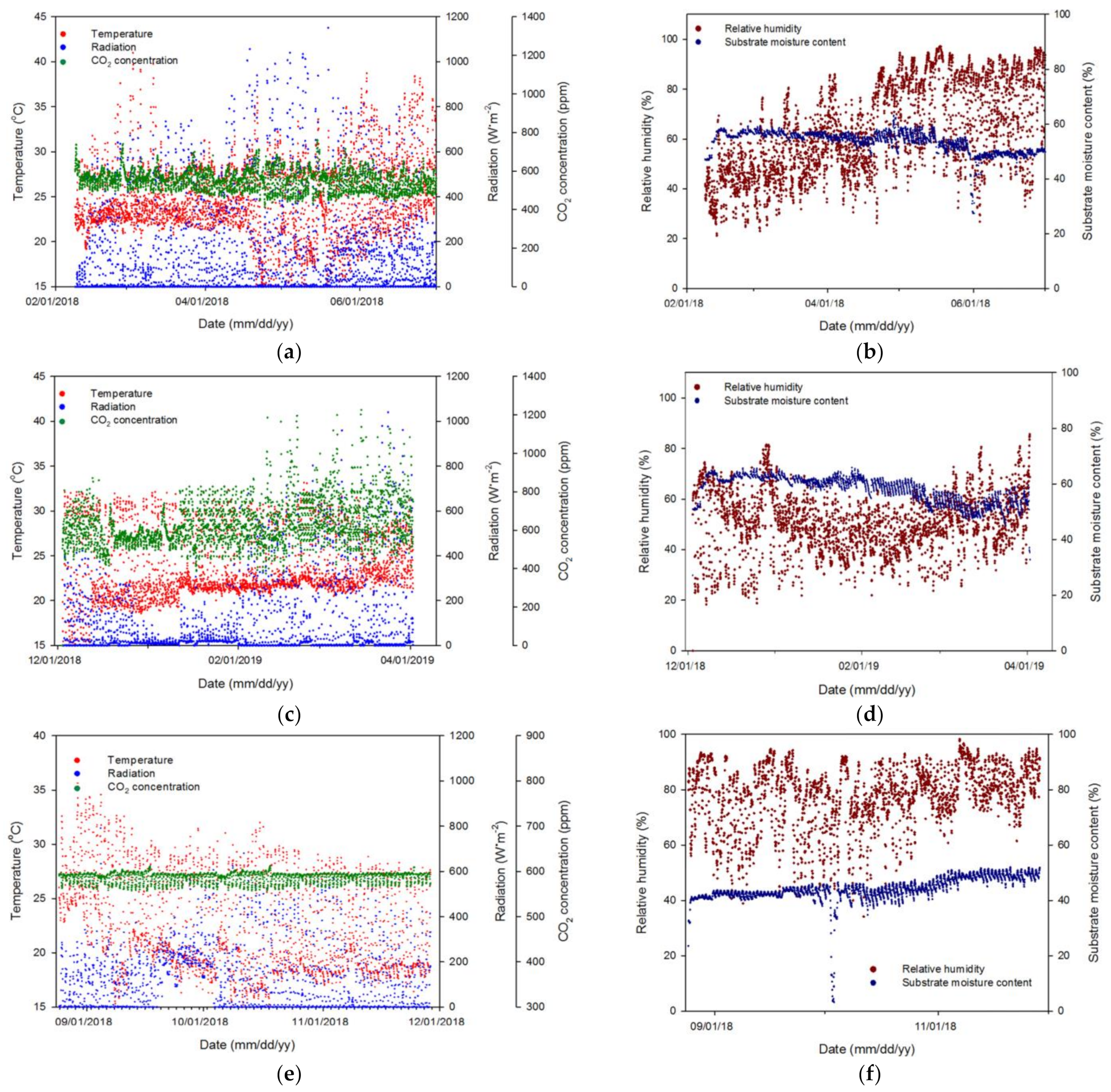
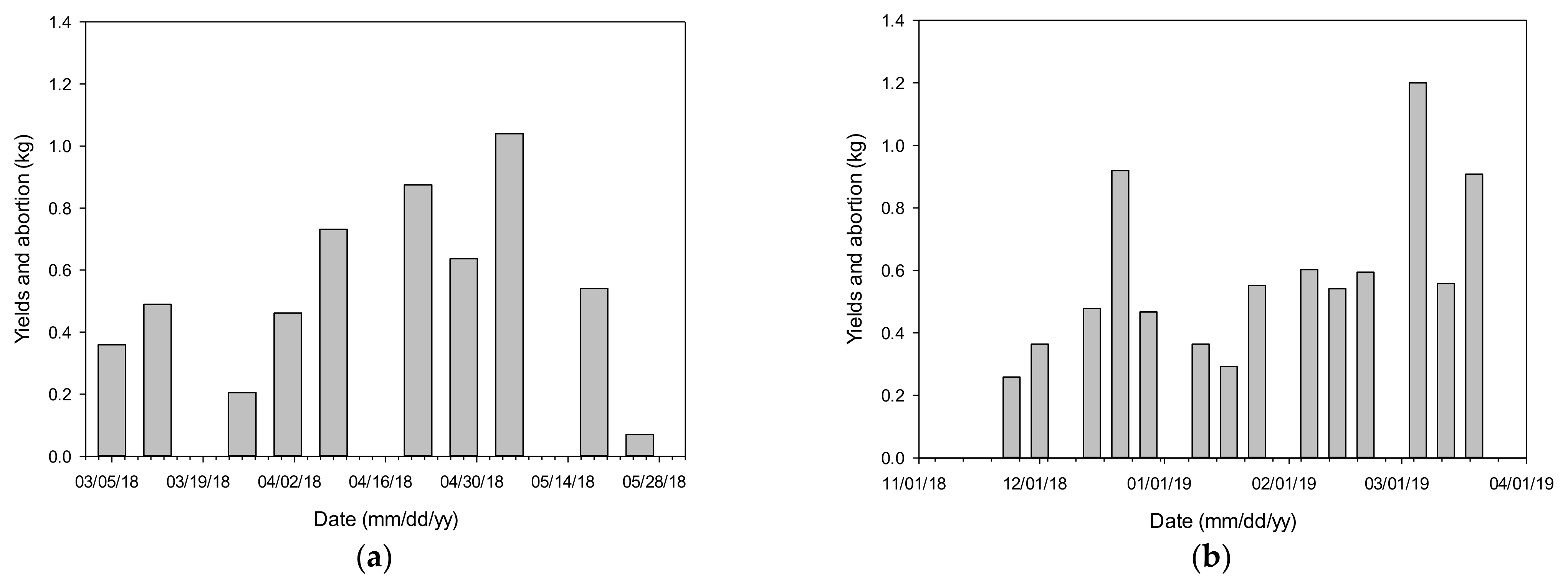
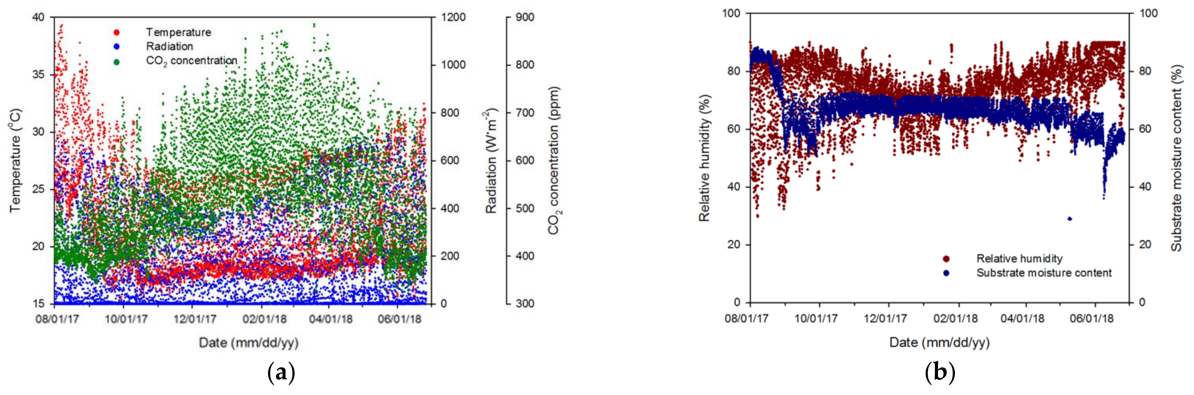
3.1. Variable Collection for Algorithm Training

Environmental data in the greenhouse were measured during three growth periods (1 September 2018–1 December 2018 for growth period 1; 1 December 2018–1 April 2019 for growth period 2; and 1 February 2018–1 June 2018 for growth period 3) as shown in Figure 2. The fruit yield and the abortion weight of the crop measured as fresh weight are shown in Figure 3. In growth period 3, the fruits were kept without harvest until the end of the data collection. The RNN algorithm estimated crop growth rate as negative because the fruit harvest caused a drastic reduction in fresh weights. To compensate the negative effects of the total fresh weight calibrated, weight was calculated by adding the weight of harvested or aborted fruits to the current value weights [35] (Figure 4). The crop growth rate was calculated using weekly changes in the calibrated weight and was applied as an algorithm. The LAI and crop-calibrated fresh weight exhibited sigmoidal growth patterns with DAT (Figure 4). A drastic decrease in fresh weight occurred during growth period 2 (Figure 4c).

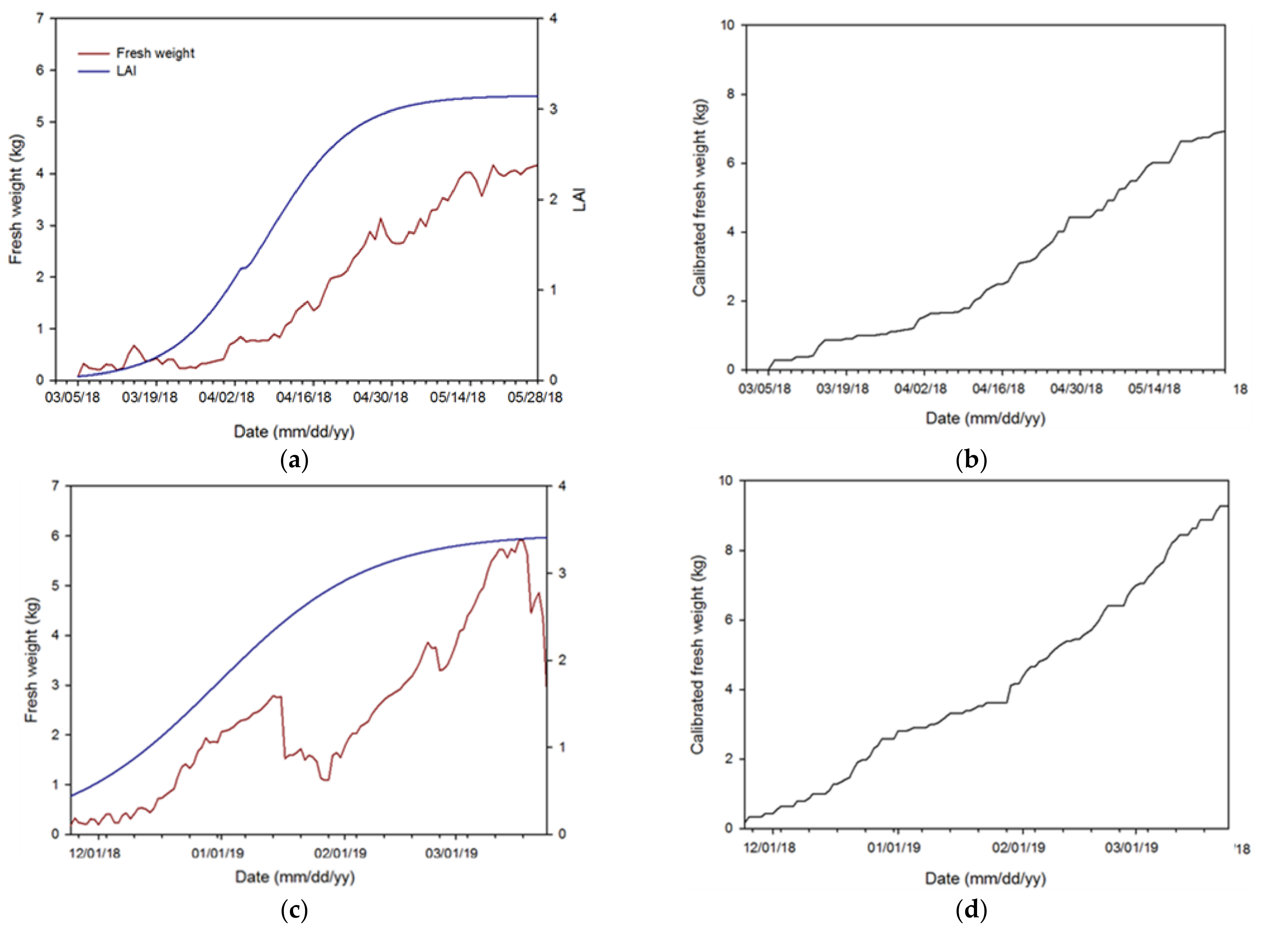
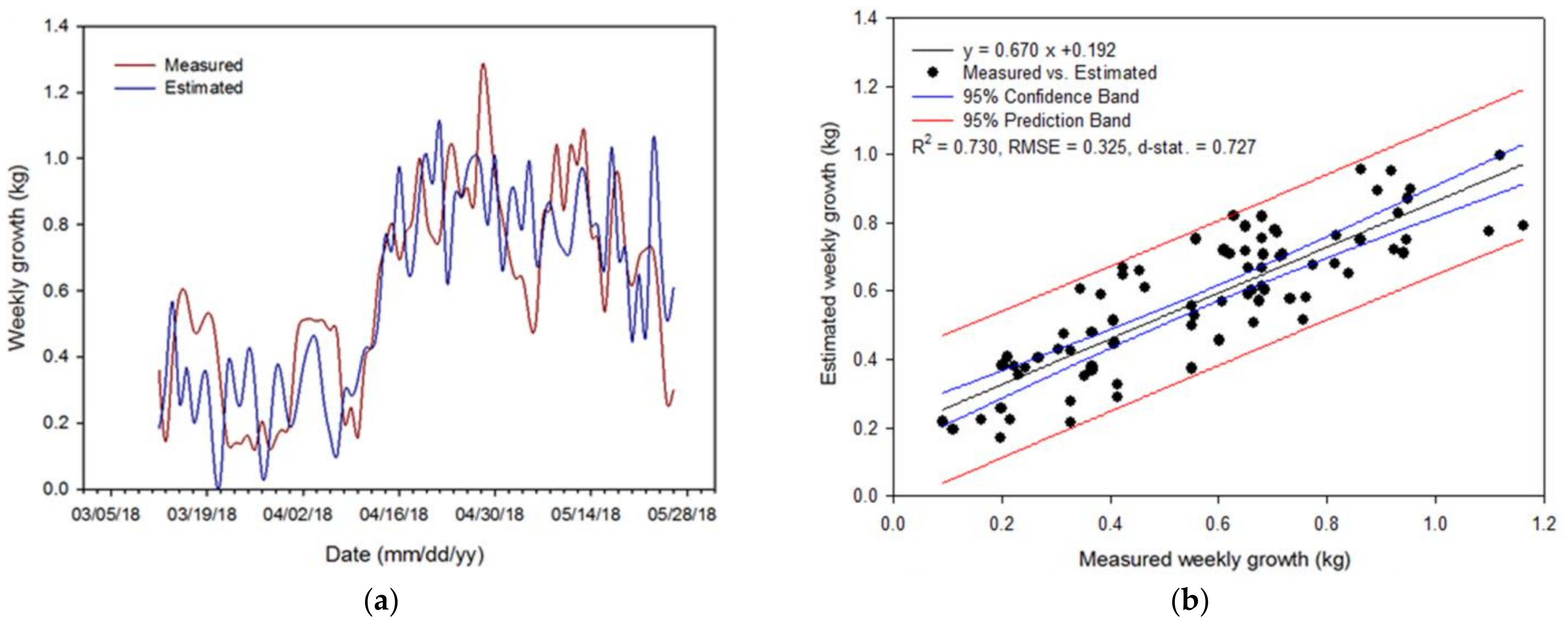
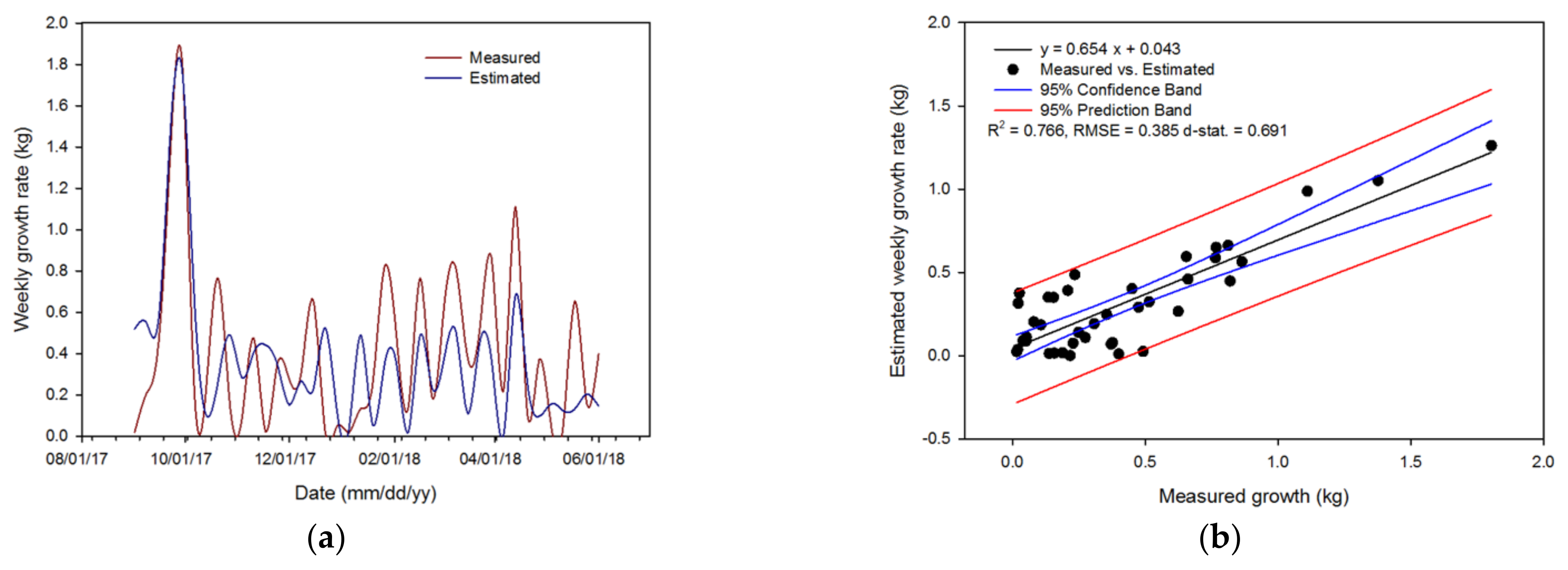
3.2. Crop Growth Rate Estimation of the Algorithm

The trained RNN algorithm estimated the actual crop growth rate similarly to the actual calibrated fresh weight (Figure 5). The d-statistic, indicating estimation accuracy, was 0.727, 0.806, and 0.748 for each growth period, respectively. From these results, the RNN algorithm could reliably estimate the actual crop growth rate. These results are similar to the previous studies that estimated the crop growth rate using ANNs [36,37,38]. While the accuracy in the previous study had been obtained by using a large amount of data from a large scale farm to train the ANN, the accuracy in this study used the data from a single greenhouse, but it was high due to the characteristics of RNN that interprets data chronologically.
During growth period 2, crop growth rate was dramatically reduced for about two weeks because the crop stem was broken (on 16 January 2019) (Figure 6). The physical injury increased the maintenance respiration [39,40], resulting in the reduction of the crop growth rate over several days. The RNN specializes in interpreting data with time intervals between input and output variables [41]. The RNN algorithm estimated the current crop growth rate based on input variables from the past week. The time interval between the input and output variables affected the estimation accuracy during crop physical injury and its recovery. The actual crop growth rate rapidly decreased after January 16 and then recovered after several days. However, the RNN algorithm estimated the growth rate higher than the actual growth rate (during 16–23 January) because the algorithm used input variables from 9–16 January. RNN, which can estimate current situations (output variables) with past data (input variables), has the advantage of analyzing the cumulative effect of environmental factors but is disadvantaged when immediately reacting to unexpected changes in conditions.

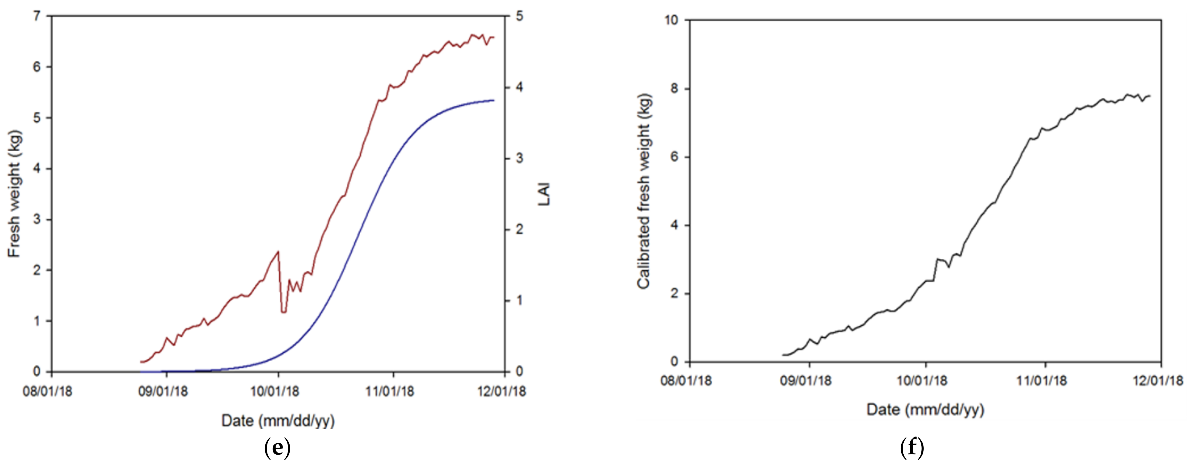
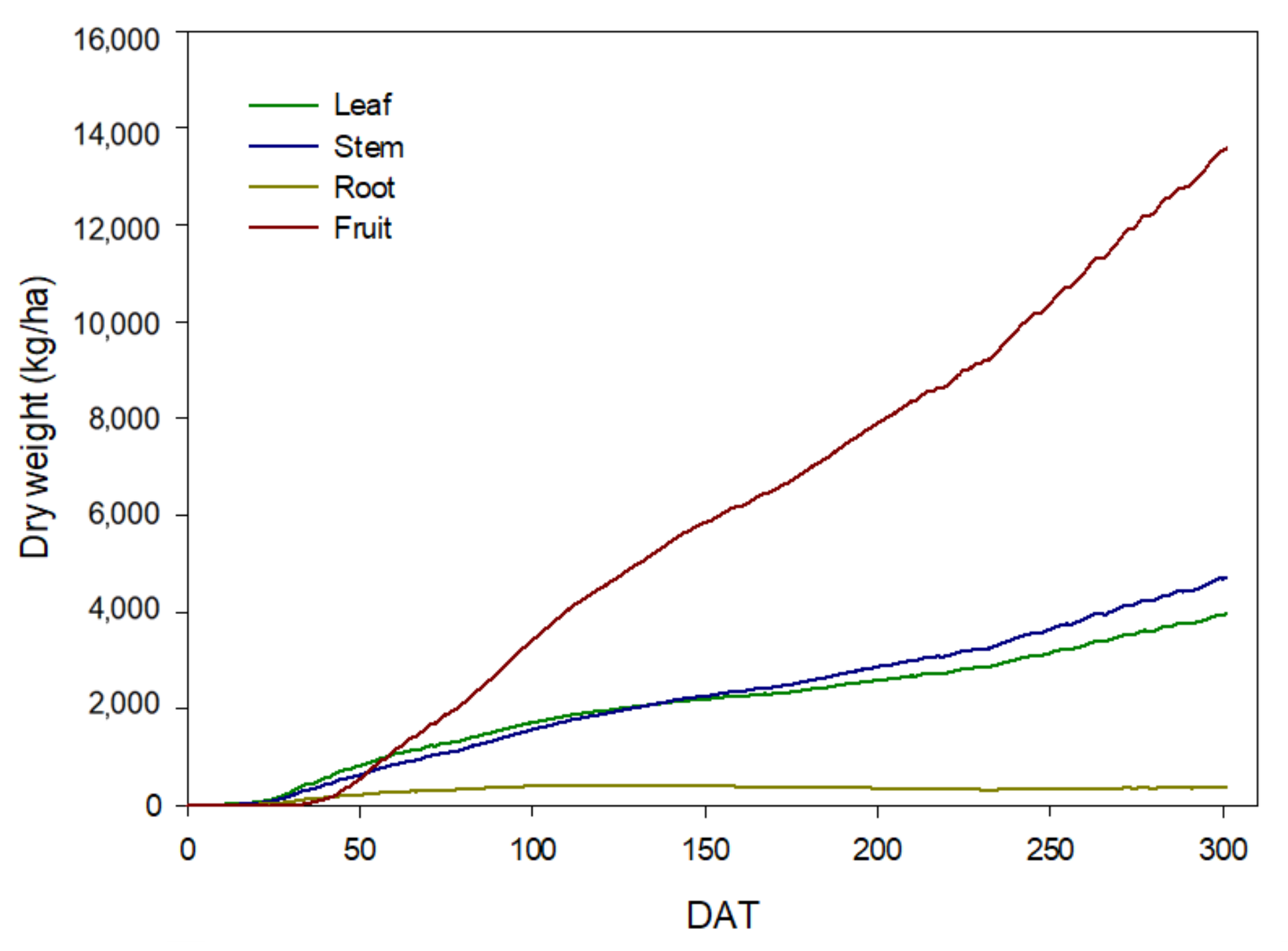
3.3. Calibration and Simulation of the PBM

The CropGro-bell pepper model was calibrated from the growth cultivation for algorithm training (Table 4 and Table 5). The automatically calculated parameters were re-calibrated to match the previous study results [42]. The crop growth is divided into seven stages in the PBM and no further growth is estimated after the crop reaches the R7 stage. Additionally, when the photothermal day is above a particular value (e.g., past 200 days after the first flowers, leaves no longer expand [42]), it estimated that the growing point no longer develops, resulting in no appearance of new nodes [43]. However, because bell pepper continuously grows until the end of the growth period in greenhouse conditions, effects of these parameters should be minimized. Boote et al. [44] revised the infinite values of SD-PM, the time between the first seed (R3), physiological maturity (R7), and FL-VS (time from the first flower to the last leaf on the main stem) for greenhouse-grown tomatoes to represent the tomato growth curve as an infinite form. Therefore, SD-PM and FL-VS were set to 330 because the growth and development of bell peppers continued until the end of the measurement period.
The calibrated PBM was able to simulate the organ-specific growth of crops (Figure 7). In the early periods of the growth stage, the growth rate of roots was faster but then decreased, while the growth rate of stems and leaves continued to increase. From the first fruit development time, fruit growth was a major factor in the whole crop growth. Consequently, fruit sink strength is very high compared to that of bell pepper organs [45]. The ratio of dry–fresh weight was highest in fruits and lowest in roots (data not shown). In other crop organs, the dry–fresh weight ratio of organs did not change depending on the growth stage, except for stems for which the ratio was highest in the initial growth stage and constant from the middle growth stage. As the PBM calculated the crop growth rate based on dry weight, the fresh weight was computed with the dry–fresh weight ratio measured at every growth stage.

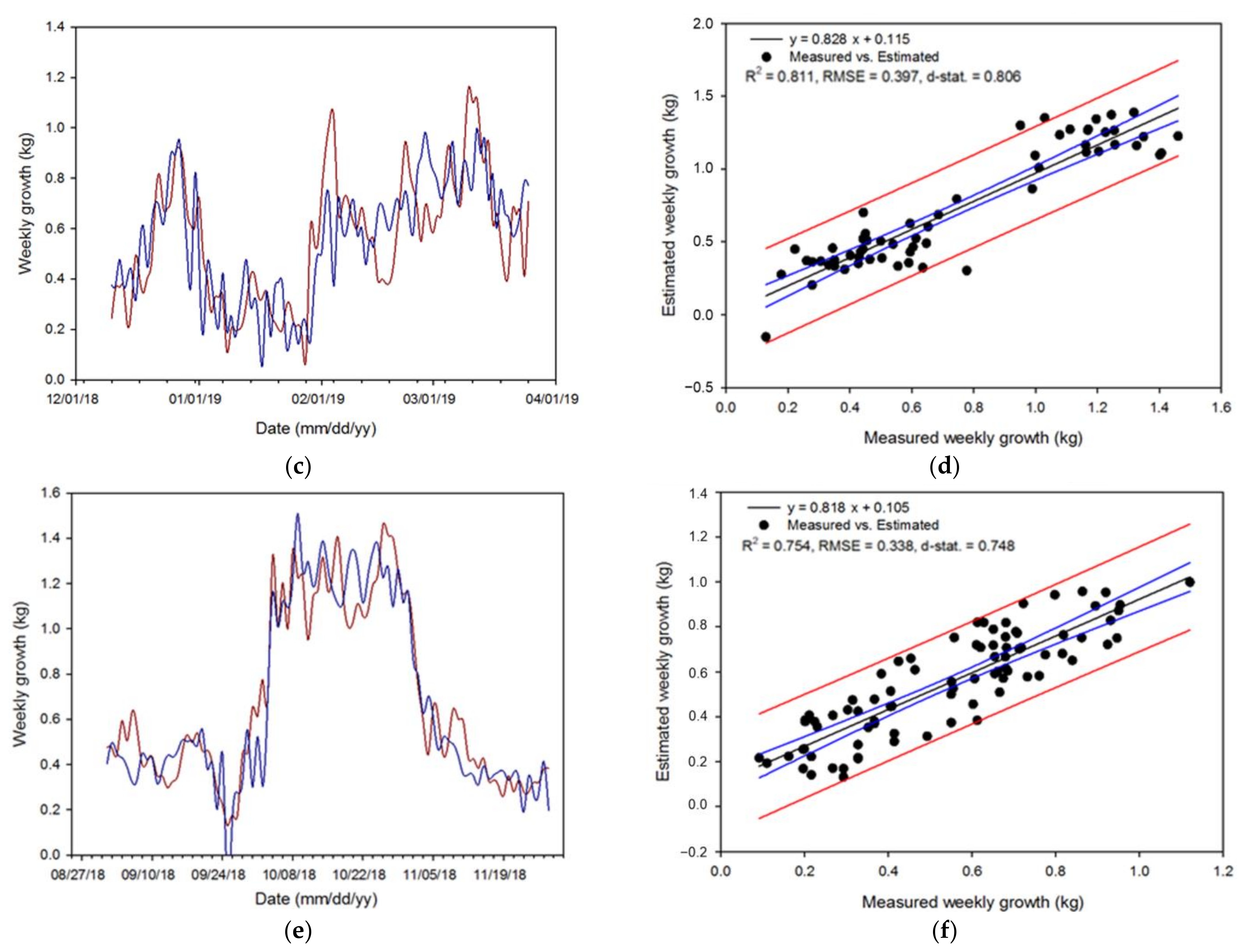
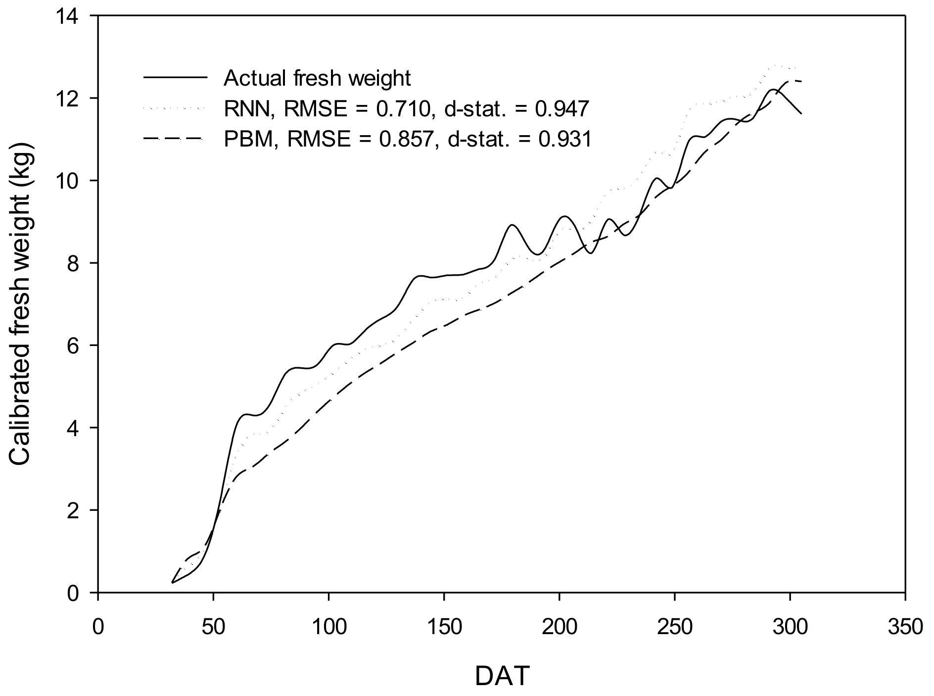
3.4. Validation and Evaluation of the Algorithm

The environmental variables collected in the validation were in the range of Figure 8. In the validation, the RNN algorithm estimated the crop growth rate with reasonable accuracy (Figure 9), although the accuracy was relatively low compared to the training test. The RNN algorithm could estimate the fresh weight with higher accuracy than the PBM (Figure 10). Furthermore, the RNN algorithm had a lower RMSE value and a higher d-statistic than the PBM. Although the amount of data used to optimize the RNN training was insufficient, the RNN algorithms developed were more accurate than the PBM. The RNN algorithm when using daily crop growth data could precisely reflect environmental conditions. In addition, the RNN algorithm estimated the crop growth for typical bell pepper cultivation periods (autumn–spring for validation), even from learning data collected during separate growth periods (winter–spring for periods 1 and 2 and autumn–winter for period 3). These results present the possibility of utilizing the data collected under various seasonal environmental conditions without necessarily continuing the completed cultivation to learn the RNN algorithm.

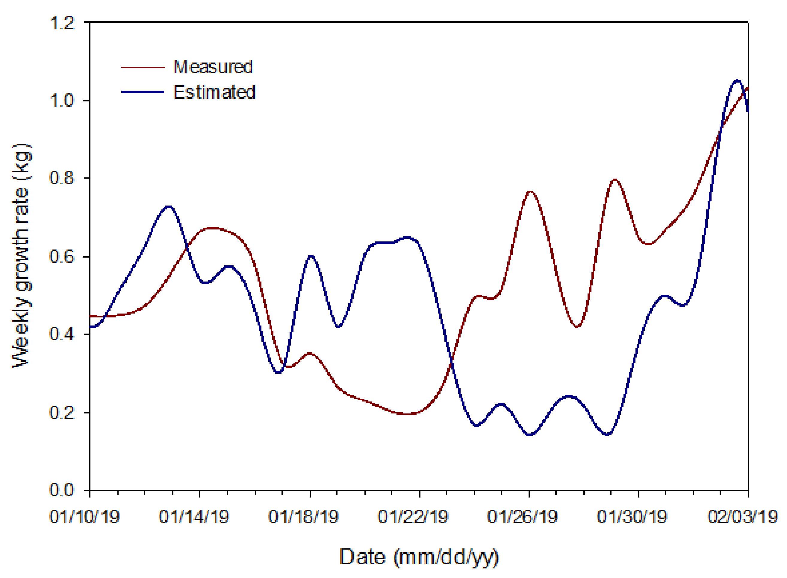
3.5. Advantages and Limitations

Due to the demands of modeling and quantitative technical demands for big data collected from smart farms [46], research on estimating crop growth using machine learning-based algorithms is being attempted [16,47,48]. In this study, it was possible to estimate the crop growth rate in a single greenhouse with a reliable accuracy level using RNN. The developed algorithm improved the estimation accuracy compared to the current machine learning algorithm [36,37,38] as well as the existing PBMs.
These studies using crop growth data also have limitations. In PBMs, the parameters of the model are determined to reflect the physiological crop characteristics. In general, the process of estimating parameters may cause specific coefficients to fall outside the normal range. However, these parameters can be altered by manually calibrating them to more realistic values. Although many studies have shown that ANNs exhibit superior predictive powers compared to conventional approaches, they do provide little explanation for the relative influence of the independent variables in the prediction process. In addition, the RNN algorithm does not provide information on the growth of specific crop organs, such as leaves, stems, and fruits. Existing PBMs estimate the total biomass by obtaining the biomass distribution to each organ [11,12] and can estimate the target organ [10]. Therefore, for the practical application of the RNN algorithm, additional research that can continuously estimate the growth rate of each organ is needed.

4. Conclusions

RNN-based algorithms were developed to estimate the crop growth response to environmental factors. An RNN algorithm was designed to estimate crop growth, consisting of six environmental variables, two crop growth factors, and DAT as input variables, and produced a weekly crop growth rate with reliable accuracy. The RNN algorithm estimated crop growth with higher accuracy than the conventional PBM in the validation. The RNN algorithm can be used to analyze the relationship between crop growth and environmental factors, and estimate crop growth with a limited number of data. The RNN algorithm developed in this study enables the quantitative analysis of crop growth for the environment in greenhouses and we expect that this method can be useful for designing optimal technologies for environmental control in greenhouses.

Author Contributions

Conceptualization, J.-W.L. and J.-E.S.; methodology, J.-W.L. and J.-E.S.; validation, J.-W.L. and T.M.; formal analysis, J.-W.L., T.M. and J.-E.S.; investigation, J.-W.L. and J.-E.S.; writing—original draft preparation, J.-W.L.; writing—review and editing, J.-E.S.; supervision, J.-E.S.; funding acquisition, J.-E.S. All authors have read and agreed to the published version of the manuscript.

Funding

This work was supported by the Research Grant of Jeonju University and IPET through the Agriculture, Food, and Rural Affairs Convergence Technologies Program for Educating Creative Global Leader (717001-7).

Institutional Review Board Statement

Not applicable.

Informed Consent Statement

Not applicable.

Data Availability Statement

Data is contained within the article.

Acknowledgments

We thank Doo-Sung Nam for his cooperation with the data analysis, collection, and crop management.

Conflicts of Interest

The authors declare no conflict of interest.

References

  1. Atzberger, C. Advances in remote sensing of agriculture: Context description, existing operational monitoring systems and major information needs. Remote Sens. 2013, 5, 949–981. [Google Scholar] [CrossRef] [Green Version]
  2. Zamora-Izquierdo, M.A.; Santa, J.; Martínez, J.A.; Martínez, V.; Skarmeta, A.F. Smart farming IoT platform based on edge and cloud computing. Biosyst. Eng. 2019, 177, 4–17. [Google Scholar] [CrossRef]
  3. Baoyun, W. Review on internet of things. J. Electron. Meas. Instrum. 2009, 12, 1–7. [Google Scholar]
  4. Chi, M.; Plaza, A.; Benediktsson, J.A.; Sun, Z.; Shen, J.; Zhu, Y. Big data for remote sensing: Challenges and opportunities. Proc. IEEE 2016, 104, 2207–2219. [Google Scholar] [CrossRef]
  5. Sonka, S. Big data: Fueling the next evolution of agricultural innovation. J. Innov. Manag. 2016, 4, 114–136. [Google Scholar] [CrossRef]
  6. Wolfert, S.; Ge, L.; Verdouw, C.; Bogaardt, M.J. Big data in smart farming—A review. Agric. Syst. 2017, 153, 69–80. [Google Scholar] [CrossRef]
  7. Kamilaris, A.; Kartakoullis, A.; Prenafeta-Boldú, F.X. A review on the practice of big data analysis in agriculture. Comput. Electron. Agric. 2017, 143, 23–37. [Google Scholar] [CrossRef]
  8. Jones, J.W.; Antle, J.M.; Basso, B.; Boote, K.J.; Conant, R.T.; Foster, I.; Godfray, H.C.J.; Herrerog, M.; Howitth, R.E.; Janssen, S.; et al. Brief history of agricultural systems modeling. Agric. Syst. 2017, 155, 240–254. [Google Scholar] [CrossRef]
  9. Dayan, E.; Van Keulen, H.; Jones, J.W.; Zipori, I.; Shmuel, D.; Challa, H. Development, calibration and validation of a greenhouse tomato growth model: I. Description of the model. Agric. Syst. 1993, 43, 145–163. [Google Scholar] [CrossRef]
  10. Marcelis, L.F.M.; Heuvelink, E.; Goudriaan, J. Modelling biomass production and yield of horticultural crops: A Review. Sci. Hortic. 1998, 74, 83–111. [Google Scholar] [CrossRef]
  11. Heuvelink, E. Evaluation of a dynamic simulation model for tomato crop growth and development. Ann. Bot. 1999, 83, 413–422. [Google Scholar] [CrossRef] [Green Version]
  12. Martínez-Ruiz, A.; López-Cruz, I.L.; Ruiz-García, A.; Pineda-Pineda, J.; Prado-Hernández, J.V. HortSyst: A dynamic model to predict growth, nitrogen uptake, and transpiration of greenhouse tomatoes. Chil. J. Agric. Res. 2019, 79, 89–102. [Google Scholar] [CrossRef] [Green Version]
  13. Wang, L. A hybrid genetic algorithm-neural network strategy for simulation optimization. Appl. Math. Comput. 2005, 170, 1329–1343. [Google Scholar] [CrossRef]
  14. LeCun, Y.; Bengio, Y.; Hinton, G. Deep learning. Nature 2015, 521, 436–444. [Google Scholar] [CrossRef]
  15. Arab, M.M.; Yadollahi, A.; Shojaeiyan, A.; Ahmadi, H. Artificial neural network genetic algorithm as powerful tool to predict and optimize in vitro proliferation mineral medium for g × n15 rootstock. Front. Plant Sci. 2016, 7, 1526. [Google Scholar] [CrossRef] [Green Version]
  16. Ehret, D.L.; Hill, B.D.; Helmer, T.; Edwards, D.R. Neural network modeling of greenhouse tomato yield, growth and water use from automated crop monitoring data. Comput. Electron. Agric. 2011, 79, 82–89. [Google Scholar] [CrossRef]
  17. Küçükönder, H.; Boyaci, S.; Akyüz, A. A modeling study with an artificial neural network: Developing estimation models for the tomato plant leaf area. Turk. J. Agric For. 2016, 40, 203–212. [Google Scholar] [CrossRef]
  18. Adavanne, S.; Parascandolo, G.; Pertilä, P.; Heittola, T.; Virtanen, T. Sound event detection in multichannel audio using spatial and harmonic features. arXiv 2017, arXiv:1706.02293. [Google Scholar]
  19. Ororbia, A.G., II; Mikolov, T.; Reitter, D. Learning simpler language models with the differential state framework. Neural Comput. 2017, 29, 3327–3352. [Google Scholar] [CrossRef] [Green Version]
  20. Hochreiter, S.; Schmidhuber, J. Long short-term memory. Neural Comput. 1997, 9, 1735–1780. [Google Scholar] [CrossRef]
  21. Jung, D.H.; Kim, H.S.; Jhin, C.; Kim, H.J.; Park, S.H. Time-serial analysis of deep neural network models for prediction of climatic conditions inside a greenhouse. Comput. Electron. Agric. 2020, 173, 105402. [Google Scholar] [CrossRef]
  22. Moon, T.; Ahn, T.I.; Son, J.E. Long short-term memory for a model-free estimation of macronutrient ion concentrations of root-zone in closed-loop soilless cultures. Plant Methods 2019, 15, 1–12. [Google Scholar] [CrossRef] [Green Version]
  23. Mouatadid, S.; Adamowski, J.F.; Tiwari, M.K.; Quilty, J.M. Coupling the maximum overlap discrete wavelet transform and long short-term memory networks for irrigation flow forecasting. Agric. Water Manag. 2019, 219, 72–85. [Google Scholar] [CrossRef]
  24. Jovicich, E.; Cantliffe, D.J.; Stoffella, P.J.; Haman, D.Z. Bell pepper fruit yield and quality as influenced by solar radiation-based irrigation and container media in a passively ventilated greenhouse. HortScience 2007, 42, 642–652. [Google Scholar] [CrossRef] [Green Version]
  25. Lee, J.; Moon, T.; Nam, D.S.; Park, K.S.; Son, J.E. Estimation of leaf area in paprika based on leaf length, leaf width, and node number using regression models and an artificial neural network. Hortic. Sci. Technol. 2018, 36, 183–192. [Google Scholar]
  26. Lee, J.W.; Son, J.E. Nondestructive and continuous fresh weight measurements of bell peppers grown in soilless culture systems. Agronomy 2019, 9, 652. [Google Scholar] [CrossRef] [Green Version]
  27. Bock, S.; Goppold, J.; Weiß, M. An improvement of the convergence proof of the ADAM-optimizer. arXiv 2018, arXiv:1804.10587. [Google Scholar]
  28. Kohavi, R.; George, H.J. Automatic parameter selection by minimizing estimated error. In Machine Learning Proceedings 1995; Morgan Kaufmann: Burlington, MA, USA, 1995; pp. 304–312. [Google Scholar]
  29. Jones, J.W.; Dayan, E.; Allen, L.H.; Van Keulen, H.; Challa, H. A dynamic tomato growth and yield model (TOMGRO). Trans. ASABE 1991, 34, 0663–0672. [Google Scholar] [CrossRef]
  30. Shi, Y.; Li, Y.N.; Zhang, C.; Bai, M.J.; Wang, Y.K. Development and application of decision support system for agro-technology transfer DSSAT under water resources management. Adv. Mater. Res. 2015, 1073, 1596–1603. [Google Scholar] [CrossRef]
  31. Ratto, M.; Tarantola, S.; Saltelli, A. Sensitivity analysis in model calibration: GSA-GLUE approach. Comput. Phys. Commun. 2001, 136, 212–224. [Google Scholar] [CrossRef]
  32. Jones, J.W.; Hoogenboom, G.; Porter, C.H.; Boote, K.J.; Batchelor, W.D.; Hunt, L.A.; Wilkens, P.W.; Singh, U.; Gijsman, A.J.; Ritchie, J.T. The DSSAT cropping system model. Eur. J. Agron. 2003, 18, 235–265. [Google Scholar] [CrossRef]
  33. Hoogenboom, G.; Jones, J.W.; Traore, P.C.; Boote, K.J. Experiments and data for model evaluation and application. In Improving Soil Fertility Recommendations in Africa Using the Decision Support System for Agrotechnology Transfer (DSSAT); Springer: Dordrecht, The Netherlands, 2012; pp. 9–18. [Google Scholar]
  34. Willmott, C.J.; Robeson, S.M.; Matsuura, K. A refined index of model performance. Int. J. Climatol. 2012, 32, 2088–2094. [Google Scholar] [CrossRef]
  35. Ćosić, M.; Stričević, R.; Djurović, N.; Moravčević, D.; Pavlović, M.; Todorović, M. Predicting biomass and yield of sweet pepper grown with and without plastic film mulching under different water supply and weather conditions. Agric. Water Manag. 2017, 188, 91–100. [Google Scholar] [CrossRef]
  36. Kaul, M.; Hill, R.L.; Walthall, C. Artificial neural networks for corn and soybean yield prediction. Agric. Syst. 2005, 85, 1–18. [Google Scholar] [CrossRef]
  37. Pantazi, X.E.; Moshou, D.; Alexandridis, T.; Whetton, R.L.; Mouazen, A.M. Wheat yield prediction using machine learning and advanced sensing techniques. Comput. Electron. Agric. 2016, 121, 57–65. [Google Scholar] [CrossRef]
  38. Teimouri, N.; Dyrmann, M.; Nielsen, P.; Mathiassen, S.; Somerville, G.; Jørgensen, R. Weed growth stage estimator using deep convolutional neural networks. Sensors 2018, 18, 1580. [Google Scholar] [CrossRef] [PubMed] [Green Version]
  39. Toyota, M.; Spencer, D.; Sawai-Toyota, S.; Jiaqi, W.; Zhang, T.; Koo, A.J.; Howe, G.A.; Gilroy, S. Glutamate triggers long-distance, calcium-based plant defense signaling. Science 2018, 361, 1112–1115. [Google Scholar] [CrossRef] [PubMed]
  40. Fonseca, S.C.; Oliveira, F.A.; Brecht, J.K. Modelling respiration rate of fresh fruits and vegetables for modified atmosphere packages: A review. J. Food Eng. 2002, 52, 99–119. [Google Scholar] [CrossRef]
  41. Jozefowicz, R.; Zaremba, W.; Sutskever, I. An empirical exploration of recurrent network architectures. In Proceedings of the International Conference on Machine Learning, Lille, France, 6–11 July 2015; pp. 2342–2350. [Google Scholar]
  42. Csizinszky, A.A. Yield and nutrient uptake of Capistrano bell peppers in compost-amended sandy soil. Proc. Fla. State Hortic. Soc. 1999, 112, 333–336. [Google Scholar]
  43. Boote, K.J.; Jones, J.W.; Hoogenboom, G.; Pickering, N.B. Simulation of crop growth: CROPGRO model. Agric. Syst. 1998, 18, 651–692. [Google Scholar]
  44. Boote, K.J.; Rybak, M.R.; Scholberg, J.M.; Jones, J.W. Improving the CROPGRO-tomato model for predicting growth and yield response to temperature. HortScience 2012, 47, 1038–1049. [Google Scholar] [CrossRef]
  45. Vieira, M.I.; de Melo-Abreu, J.P.; Ferreira, M.E.; Monteiro, A.A. Dry matter and area partitioning, radiation interception and radiation-use efficiency in open-field bell pepper. Sci. Hortic. 2009, 121, 404–409. [Google Scholar] [CrossRef] [Green Version]
  46. Hashem, I.A.T.; Yaqoob, I.; Anuar, N.B.; Mokhtar, S.; Gani, A.; Khan, S.U. The rise of “big data” on cloud computing: Review and open research issues. Inf. Syst. 2015, 47, 98–115. [Google Scholar] [CrossRef]
  47. Gupta, D.K.; Kumar, P.; Mishra, V.N.; Prasad, R.; Dikshit, P.K.S.; Dwivedi, S.B.; Ohri, A.; Singh, R.S.; Srivastava, V. Bistatic measurements for the estimation of rice crop variables using artificial neural network. Adv. Space Res. 2015, 55, 1613–1623. [Google Scholar] [CrossRef]
  48. Kumar, K.; Kumar, S.; Sankar, V.; Sakthivel, T.; Karunakaran, G.; Tripathi, P.C. Non-destructive estimation of leaf area of durian (Durio zibethinus)–An artificial neural network approach. Sci. Hortic. 2017, 219, 319–325. [Google Scholar]
Figure 1. A schematic diagram of the fresh weight measuring system using the load cell and frequency domain reflectometry (FDR) sensors (a), and the actual installation of the fresh weight measuring system (b).
Horticulturae 07 00284 g001
Figure 2. Environmental conditions (temperature, radiation, and CO2 concentration) in the greenhouse during growth period 1 (1 February 2018–1 June 2018) (a,b); growth period 2 (1 December 2018–1 April 2019) (c,d); and growth period 3 (1 September 2018–1 December 2018) (e,f).
Horticulturae 07 00284 g002
Figure 3. The weight of fruit yield and abortion at one-week intervals during growth period 1 (1 February 2018–1 June 2018) (a) and growth period 2 (1 December 2018–1 April 2019) (b).
Horticulturae 07 00284 g003
Figure 4. Changes in fresh weight and LAI (a) as well as in the calibrated fresh weight (b) during growth period 1 (1 February 2018–1 June 2018); changes in fresh weight and LAI (c) as well as in the calibrated fresh weight (d) during growth period 2 (1 December 2018–1 April 2019); and changes in fresh weight and LAI (e) as well as in the calibrated fresh weight (f) during growth period 3 (1 September 2018–1 December 2018).
Horticulturae 07 00284 g004aHorticulturae 07 00284 g004b
Figure 5. Comparison of the weekly crop growth rate measured by the fresh weight measuring system and estimated by the recurrent neural network (RNN) algorithm during growth period 1 (1 February 2018–1 June 2018) (a,b); growth period 2 (1 December 2018–1 April 2019) (c,d); and growth period 3 (1 September 2018–1 December 2018) (e,f).
Horticulturae 07 00284 g005aHorticulturae 07 00284 g005b
Figure 6. Comparison of the weekly crop growth rates measured by the fresh weight measuring system and estimated by the recurrent neural network (RNN) algorithm during the growth period from 10 January 2019 to 3 February 2019.
Horticulturae 07 00284 g006
Figure 7. Dry weight of each organ estimated by the process-based model (PBM) with days after transplanting (DAT).
Horticulturae 07 00284 g007
Figure 8. Environmental conditions in the greenhouse during validation periods from 1 August 2017 to 1 June 2018. Temperature, radiation, and CO2 concentration (a), and relative humidity and substrate moisture content (b).
Horticulturae 07 00284 g008
Figure 9. Comparison of the weekly crop growth rates measured by the fresh weight measuring system and estimated by the recurrent neural network (RNN) algorithm during the growth period from 1 August 2017 to 1 June 2018 for validation cultivation (a). The test accuracies of the algorithms (b).
Horticulturae 07 00284 g009
Figure 10. Comparison of the calibrated fresh weights estimated by the recurrent neural network (RNN) algorithm and the process-based model (PBM) with days after transplanting (DAT) in growth validation periods.
Horticulturae 07 00284 g010
Table 1. Hyperparameters for the recurrent neural network (RNN) and AdamOptimizer.
ParameterValueDescription
Learning rate0.001Learning rate used by the AdamOptimizer
β10.9Exponential mass decay rate for the momentum estimates
β20.999Exponential velocity decay rate for the momentum estimates
E1 × 10−0.8A constant for numerical stability
Forget bias1.0Probability of forgetting information in the previous dataset
Time step2–24Number of datasets that the LSTM sees at one time
Table 2. Genotype coefficients of bell pepper in CropGro-pepper.
IndexDescription (Unit)
PPSENSlope of the relative response of development to photoperiod with time (positive for short-day plants) (1/h)
EM-FLTime between plant emergence and flower appearance (R1) (photothermal days)
FL-SHTime between first flower and first pod (R3) (photothermal days)
FL-SDTime between first flower and first seed (R5) (photothermal days)
SD-PMTime between first seed (R5) and physiological maturity (R7) (photothermal days)
FL-LFTime between first flower (R1) and end of leaf expansion (photothermal days)
LFMAXMaximum leaf photosynthesis rate at 30 °C, 350 vpm CO2, and high light (mg CO2/m2/s)
SLAVRSpecific leaf area of cultivar under standard growth conditions (cm2/g)
SIZLFMaximum size of full leaf (three leaflets) (cm2)
CSDLCritical short day length below which reproductive development progresses with no daylength effect (for short-day plants) (hour)
XFRTMaximum fraction of daily growth that is partitioned to seed + shell
WTPSDMaximum weight per seed (g)
SFDURSeed filling duration for pod cohort at standard growth conditions (photothermal days)
SDPDVAverage seed per pod under standard growing conditions (#/pod)
PODURTime required for cultivar to reach final pod load under optimal conditions (photothermal days)
THRSHThreshing percentage: the maximum ratio of (seed/(seed + shell)) at maturity
SDPROFraction protein in seeds (g(protein)/g(seed))
SDLIPFraction oil in seeds (g(oil)/g(seed))
Table 3. Ecotype coefficients of bell pepper in CropGro-pepper.
IndexDescription (Unit)
MGMaturity group number for this ecotype, such as maturity group
TMIndicator of temperature adaptation
THVARMinimum rate of reproductive development under short days
PL-EMTime between planting and emergence (V0), thermal days
EM-V1Time required from emergence to first true leaf (V1), thermal days
V1-JUTime required from first true leaf to end of juvenile phase, thermal days
JU-R0Time required for floral induction, equal to the minimum number of days for floral induction under optimal temperature and daylengths, photothermal days
PM06Proportion of time between first flower and first pod for first peg
PM09Proportion of time between first seed and physiological maturity in which the last seed may be formed
LNGSHTime required for growth of individual shells (photothermal days)
R7-R8Time between physiological (R7) and harvest maturity (R8) (days)
FL-VSTime from first flower to last leaf on main stem (photothermal days)
TRIFOLRate of appearance of leaves on the mainstem (leaves per thermal day)
RWIDTHRelative width of this ecotype in comparison to the standard width per node
RHGHTRelative height of this ecotype in comparison to the standard height per node
R1PPOIncrease in daylength sensitivity after R1 (h)
OPTBIMinimum daily temperature above which there is no effect on slowing normal development towards flowering (°C)
SLOBISlope of relationship reducing progress towards flowering if TMIN for the day is less than OPTBI
Table 4. Calibrated genotype coefficients of bell pepper in CropGro-pepper.
IndexValueIndexValue
PPSEN0CSDL12.33
EM-FL40XFRT0.6
FL-SH10WTPSD0.007
FL-SD15SFDUR40
SD-PM330SDPDV150
FL-LF200PODUR42
LFMAX0.98THRSH6.5
SLAVR275SDPRO0.3
SIZLF350SDLIP0.05
Table 5. Calibrated ecotype coefficients of bell pepper in CropGro-pepper.
IndexValueIndexValue
MG1LNGSH35
TM1R7-R80
THVAR0FL-VS330
PL-EM5TRIFOL0.35
EM-V110RWIDTH1
V1-JU24RHGHT1
JU-R05R1PPO0
PM060OPTBI0
PM090SLOBI0
Publisher’s Note: MDPI stays neutral with regard to jurisdictional claims in published maps and institutional affiliations.

