Abstract
In subtropical regions, tomato (Solanum lycopersicum) is mainly produced in autumn and winter. To enhance the off-season production of tomato, summer cultivation has become a prime objective. Grafting tomato scions onto eggplant (Solanum melongena) rootstocks is a key method to overcome the difficulties of tomato cultivation in summer. In this study, we collected seedling growth data over six growing seasons in Taiwan and established growth models by employing three commonly used sigmoid growth curves, namely the Gompertz, Richards, and Logistic curves. Cumulative temperature was introduced as an independent variable and its relationship with plant stem diameter determined. The R2 values of the growth models were 0.74–0.85 and 0.72–0.80 in calibration and validation, respectively. Performance did not differ markedly among models in the same growing season, but notable differences were observed among models for different growing seasons. In addition, the estimates of several model parameters differed significantly among the seasons; hence, separate models should be established for different seasons. The results of this study can be used in prediction of tomato and eggplant seedling growth and arrangement of the grafting schedule to improve the efficiency of seedling production in subtropical countries.
1. Introduction
Tomato (Solanum lycopersicum) is a key crop in tropical and subtropical regions. Tomatoes are rich in nutrients, such as vitamin A, vitamin C, lycopene, and carotenoids [1,2,3]. Appropriate consumption of tomatoes can help reduce the incidence of many diseases [4]. According to the Food and Agriculture Organization of the United Nations, tomato crops accounted for 5 million ha of cultivated land worldwide and a gross output of 180.8 million Mg in 2019. According to Taiwanese government statistics, tomatoes occupied approximately 4300 ha of cultivated land in Taiwan during 2019, with an output valued at nearly USD 130 million. As tomatoes are native to Andes Mountains in South America, they are typically produced during autumn and winter in subtropical regions. Due to the concentration of the production period, market price decreases and severe supply shortages occur in summer. Therefore, summer cultivation and production of tomatoes have become key goals of the agricultural industry. However, the high summer temperatures and humidity in subtropical regions as well as the severe damage caused by diseases and pests hamper the cultivation of tomatoes in summer.
Grafting, the union of two plant parts—namely, a rootstock and a scion—is a technique for combining the genetic materials of two plants [5]. Grafting technology is currently popular and is commonly applied to Solanaceae and Cucurbitaceae crops [6,7]. Grafting is a method of preventing soilborne diseases [8,9,10,11]. Therefore, grafting crops that are susceptible to disease onto more disease-resistant crops is frequently performed to reduce the risk of plant infection [12]. For tomato, bacterial wilt (Ralstonia solanacearum) and Fusarium wilt (Fusarium oxysporum f. sp. Lycopersici) are critical soil-borne diseases. Hence, nursery operators generally graft tomatoes onto the rootstocks of more disease-resistant crops and then sell the grafted seedlings to growers. Rootstock grafting can enhance the disease resistance of plants as well as their growth potential under abiotic stress [11,13,14,15,16]. For example, grafted fresh pepper (Capsicum annuum) have reduced the content of heavy metals, such as cadmium, iron, manganese, and zinc [17]. Grafting tomatoes can reduce cadmium-based toxicity [18]. To render summer tomato production more feasible, eggplant (Solanum melongena), which can improve plant tolerance to water stress and flooding, is often used as the grafting rootstock. Additionally, grafting tomato on eggplant can increase the yield and quality of the fruit [19,20,21]. Grafting technology has already resolved many problems in tomato production and has gradually become a routine operation in agricultural production.
Generally, three pivotal factors should be considered when grafting. The first is the choice of rootstock and scion. Different rootstock–scion combinations exhibit differing growth performance, and the genotypes of rootstock and scion also affect the compatibility of grafting. The second is the grafting method. The most commonly used method is tube grafting, which can ensure that the vascular cambia of the rootstock and scion are held in close contact. The third is the timing of grafting, which is mainly determined by the stem diameter of the scion and rootstock. For tomatoes, grafting is most effective when the stem diameter of the scion and rootstock are approximately 1.5–2.5 mm [20,22,23]. In addition, the synchronization of seedlings in nurseries is highly sensitive to temperature. Therefore, to support agricultural management, a technique that enables reliable prediction of seedling growth is necessary [24].
Mathematical modeling is a method of describing the characteristics of crop growth, with such models known as growth models [25]. Establishing a growth model is helpful in understanding the growth cycle of crops and the responses of crops to their environment. Moreover, a growth model can effectively predict critical agricultural dates, such as the optimal sowing and harvest days, aiding in work scheduling and improving the efficiency of agricultural production [26,27]. As the growth and development of crops are easily affected by many environmental factors, various physiological features are typically produced. Therefore, if a prediction model can consider environmental variables that affect crop growth, the model’s predictive ability should be improved.
By definition, in a mathematical model, if the second derivative of the function for the parameter is not zero, then the parameter is nonlinear; otherwise, it is a linear parameter [28]. In some specific areas, compared with linear growth models, nonlinear models are more parsimonious and easily described. In addition, most of the parameters in nonlinear models refer to biological characteristics, rendering the growth process of crops more easily interpretable [28]. Consequently, several studies have used nonlinear functions to establish crop growth models [28]. The sigmoid curve is a typical nonlinear model category, with models typically used to describe plant height, weight, leaf area index, nitrogen fertilizer application amount, and herbicide dosage [28,29,30]. The Gompertz [31] and Logistic [32] models are sigmoid nonlinear models commonly employed in growth analysis and have been used in growth modeling for many crops, such as squash (Cucurbita pepo) and fresh pepper [33]. The parameters in sigmoid curve models can provide effective explanations [33,34,35]. However, the Richards model [36] is more flexible than both the Gompertz and Logistic models because it can describe asymmetric growth [28].
This study assessed the timing of tomato grafting to predict when the stem diameters of the rootstock (eggplant) and scion (tomato) would reach the grafting standard. Seedling growth data were collected for a total of 3 years (six growing seasons) in Taiwan, and three commonly used nonlinear functions—the Gompertz, Logistic, and Richards models—were employed to establish growth models. Cumulative temperature was used as an independent variable to predict the growth of the stem diameters for tomato and eggplant. This study’s results can be applied to the prediction of tomato and eggplant seedling growth and the development of a grafting schedule. The present findings can improve the efficiency of tomato seedlings production in subtropical countries.
2. Materials and Methods
2.1. Data Sources
In this study, tomato (Rosada cultivar) scion and eggplant (EG203 cultivar) rootstock were seeded in plug trays filled with peat moss (BAIU036AD5E7; Peltracom, Ghent, Belgium). The seedlings were irrigated daily and fertilized with 20N-10P-20K (JR Peters Inc., Allentown, PA, USA) water-soluble fertilizer solution once a week. All experiments were executed in the nursery in Chiayi County, Taiwan. Seedlings were arranged randomly in a greenhouse covered with insect-proof nets and polyethylene film on the roof. Growth and environmental parameters were collected at the seedling stage. The investigated growth parameter was plant stem diameter, which was measured above the cotyledons of 36 randomly selected seedlings by using a Vernier caliper (Li-Ji, 56-44, China). The mean stem diameter was calculated. These measurements were performed 7–10 days after sowing and repeated every 3–4 days thereafter until the seedlings had reached the grafting standard level. The environmental parameters—air temperature (°C), relative humidity (%), and light intensity (μmol m−2 s−1)—were measured automatically every minute (and averaged every hour) using a data logger (CR300; Campbell Scientific Inc., Logan, UT, USA). In this study, the growth data of the seedlings were collected for a total of six growing seasons: spring–summer (April–August) and autumn–winter (September–March of the following year) for 2018–2020. The collected data related to a total of 1441 and 1244 tomatoes grown in spring–summer and autumn–winter, respectively, and 1566 and 1310 eggplants grown in spring–summer and autumn–winter, respectively.
2.2. Growth Model Establishment
The increase in seedling stem diameter was predicted on the basis of the cumulative mean temperature in the seedling growth environment. As crop growth can be affected by environmental conditions, we divided the spring–summer and autumn–winter seasonal growth data to establish different-season-based models. However, the data of the six growing seasons were also combined to establish a global model. The descriptive statistics of the environmental parameters of the three data sets (i.e., spring–summer, autumn–winter, and combined) are presented in Table 1. For more detailed environmental information, please refer to Table S1.

Table 1.
Descriptive statistics of the environmental parameters of each data set used in this study. Values are presented as means (standard deviations).
The first step in establishing a growth model is selecting a suitable model form. This study considered three nonlinear models—the Gompertz (Equation (1)), Logistic (Equation (2)), and Richards (Equation (3)) models—for predicting the plant stem diameter (Y) by using the cumulative temperature as a predictor variable (X).
where a denotes the asymptotic value of the dependent variable (i.e., the maximum value of the dependent variable of the model), b is the location parameter related to the initial value of the model, c is the parameter that affects the growth rate in the curve, d describes the asymmetric growth (notably, when d = 1, the Richards model degenerates to the Logistic form), and εi is the error term.
For each data set, 70% of the data were randomly selected for model training and the remaining 30% of the data were used for model validation. For the three aforementioned nonlinear models, the cumulative temperature was used as a predictor variable to fit the plant stem diameter. Ultimately, nine model variants were established and compared.
2.3. Model Assumption Verification
Before fitting a candidate model, whether the model violates assumptions, such as those of normality and variance homogeneity, has to be examined. This can be done using graphical methods or formal statistical tests [28,37]. In examining the assumptions of a model, residuals are usually applied. A residual is defined as the difference between the observed and fitted values. This study used the probability plot correlation coefficient (PPCC) to test the normality hypothesis [38]. Higher PPCCs suggested values consistent with the normality. The hypotheses of homogeneity of variance were evaluated by plotting residuals against fitted values. The residuals randomly scattering around 0 and not appearing in a megaphone shape indicates that the variance is constant.
2.4. Model Performance Evaluation
Common criteria used for model performance evaluation—the determination coefficient (R2), Akaike information criterion (AIC), root mean square error (RMSE), and mean absolute error (MAE)—were used in this study. For these criteria, the lowest values indicate the optimal model except in the case of R2, for which larger values signify higher model performance.
where SSE is the error sum of squares of the model, SST is the total sum of squares of the model, L is the likelihood function of the model, n is the number of observations, p is the number of parameters in the model, yi is the ith observation value, and ŷi is the fitted value of the ith observation.
In the validation stage, we additionally implemented the prediction of a new observation Yh at X = xh. Plugging xh into the estimated growth model, we can obtain the Ŷh to predict Yh. If we define pred = Yh − Ŷh, then the estimated standard deviation of the prediction s{pred} can be calculated by considering the variance of the distribution of Y at X = xh and the variance of sampling distribution of Ŷh. Hence, the prediction limits for a new observation at a given xh were described as follows [37]:
where t (1 − α/2; n − p) is the (1 − α/2) 100th percentile of the t distribution with n − p degrees of freedom, n is the number of observations, p is the number of parameters in the model, and s{pred} is the estimated standard deviation of the prediction.
Ŷh ± t (1 − α/2; n − p) s{pred}
2.5. Model Parameter Comparison between Two Growing Seasons
To compare the model parameters between the different-season-based models for the eggplant rootstock and tomato scion, the 95% confidence intervals of the model parameters for each growing season were calculated [26,39]. If none of the estimates from one season were within the range of the confidence intervals computed for another season, the parameter estimates differed between the two season models. By contrast, if at least one of the parameter estimates was within the confidence interval generated by another season model, then no notable difference between the two season models was indicated in terms of the model parameters.
Regarding the calculation of the parameter confidence interval, the approximate (1 − α) 100% confidence interval of the parameter was obtained as follows [37]:
where t (1 − α/2; n − p) is the (1 − α/2) 100th percentile of the t distribution with n − p degrees of freedom, n is the number of observations, p is the number of parameters in the model, and SE is the standard error of the parameter estimates.
Estimate ± t (1 − α/2; n − p) SE
2.6. Statistical Analysis
All statistical analyses were implemented using the R software, with “minpack.lm,” “ggplot2,” and “ppcc” packages used for modeling, graphing, and normality verification, respectively.
3. Results and Discussion
Nonlinear models have been used to explain the growth process of many crops [28], such as squash [33], fresh pepper [33], and sunn hemp (Crotalaria juncea) [26,39]. To identify a model that exhibits good adaptability, obeys the model assumptions, and can clearly explain the crop’s growth, a series of steps are required. In the study of Archontoulis and Miguez [28], several steps were performed, including (1) selecting suitable model types, (2) evaluating model assumptions, (3) fitting models, (4) estimating model parameters, (5) comparing model performance, (6) and model interpretation. In the present study, we employed three nonlinear models (i.e., Logistic, Gompertz, and Richards) to identify the relationship between the stem diameter and cumulative temperature.
3.1. Verifying the Model Assumptions
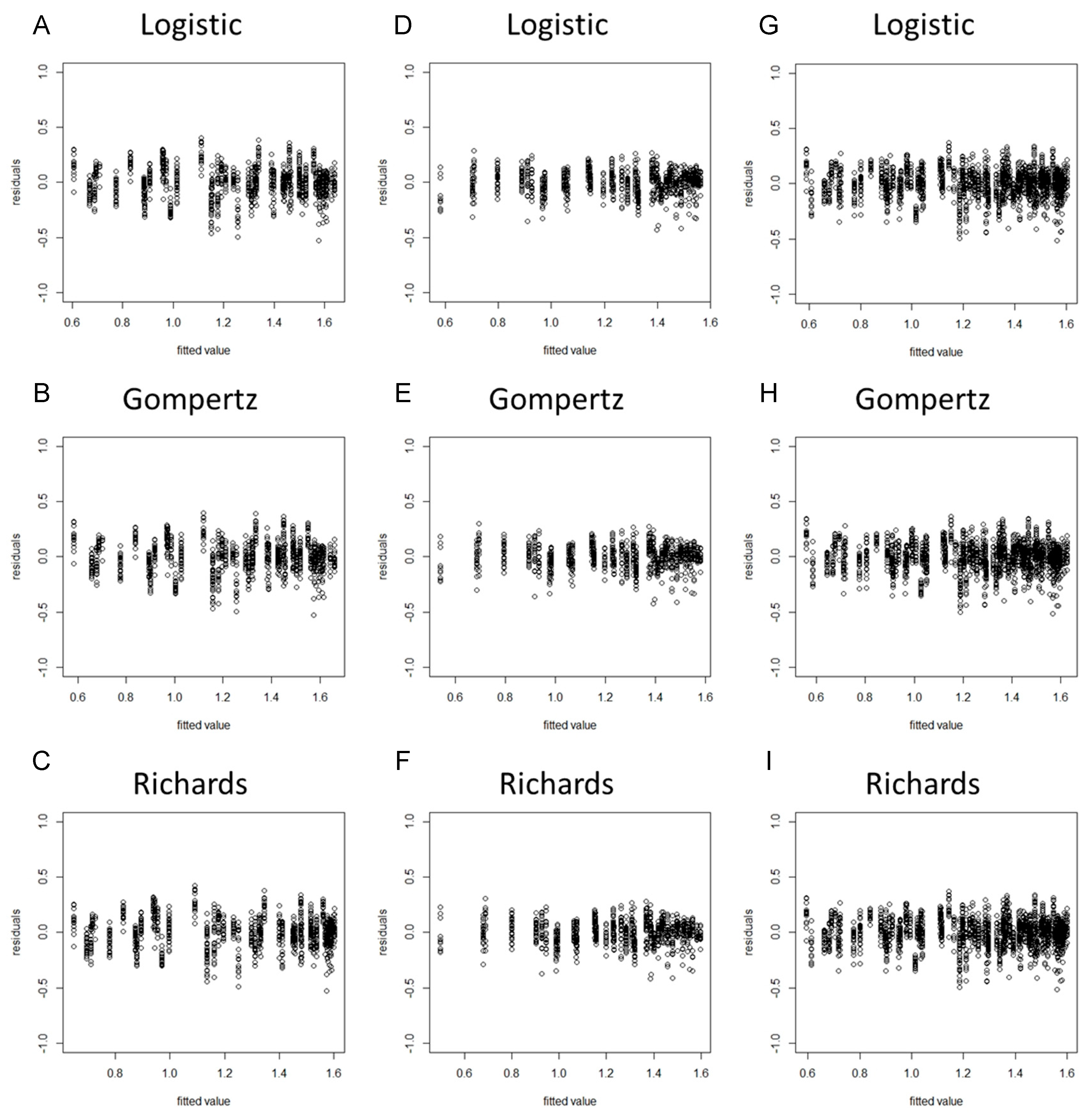
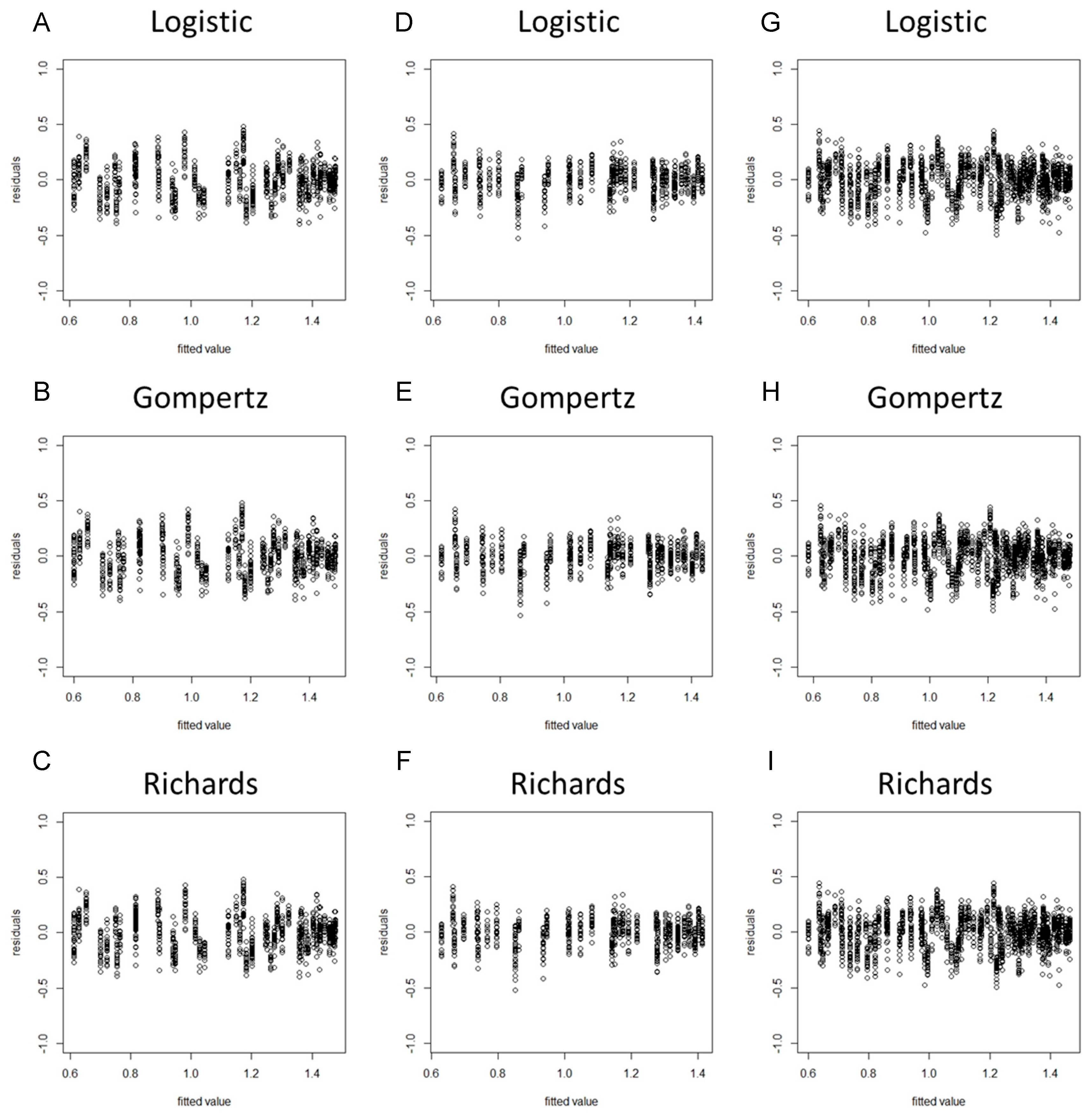
When a model is considered for an application, we usually cannot be sure in advance that the model is suitable for that application. Some of the features of the model may be violated for the particular data at hand. Hence, it is important to verify the aptness of the model for the data before inferences based on that model are made [37]. As the residuals of the fitted model (based on the original data) violated the assumptions of homogeneity of variance (Figures S1 and S2), we took the square root transformation of the stem diameter as a new dependent variable. After the variable transformation, the normality hypothesis test results suggested that the PPCC values of the nine models were all higher than 0.99 and the p-values were all less than 0.05, indicating that the model residuals obeyed the normality assumption (Table 2). The residual plots revealed that the residuals of each model did not represent specific structures or trends, suggesting that the assumption of homogeneity of variance was upheld (Figure 1 and Figure 2).

Table 2.
Results of the normality tests for the residuals of the eggplant rootstock and tomato stem diameter, based on the Logistic, Gompertz, and Richards growth models and using different seasons and combined data.
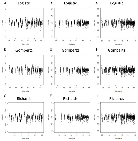
Figure 1.
Residual plots of the eggplant stem diameter by using spring−summer, autumn−winter, and combined data with the Logistic, Gompertz, and Richards growth models. (A) Spring−summer Logistic model; (B) spring−summer Gompertz model; (C) spring−summer Richards model; (D) autumn−winter Logistic model; (E) autumn−winter Gompertz model; (F) autumn−winter Richards model; (G) global Logistic model; (H) global Gompertz model; (I) global Richards model.
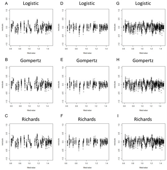
Figure 2.
Residual plots of the tomato stem diameter by using spring−summer, autumn−winter, and combined data with the Logistic, Gompertz, and Richards growth models. (A) Spring−summer Logistic model; (B) spring−summer Gompertz model; (C) spring−summer Richards model; (D) autumn−winter Logistic model; (E) autumn−winter Gompertz model; (F) autumn−winter Richards model; (G) global Logistic model; (H) global Gompertz model; (I) global Richards model.
3.2. Model Training and Validation
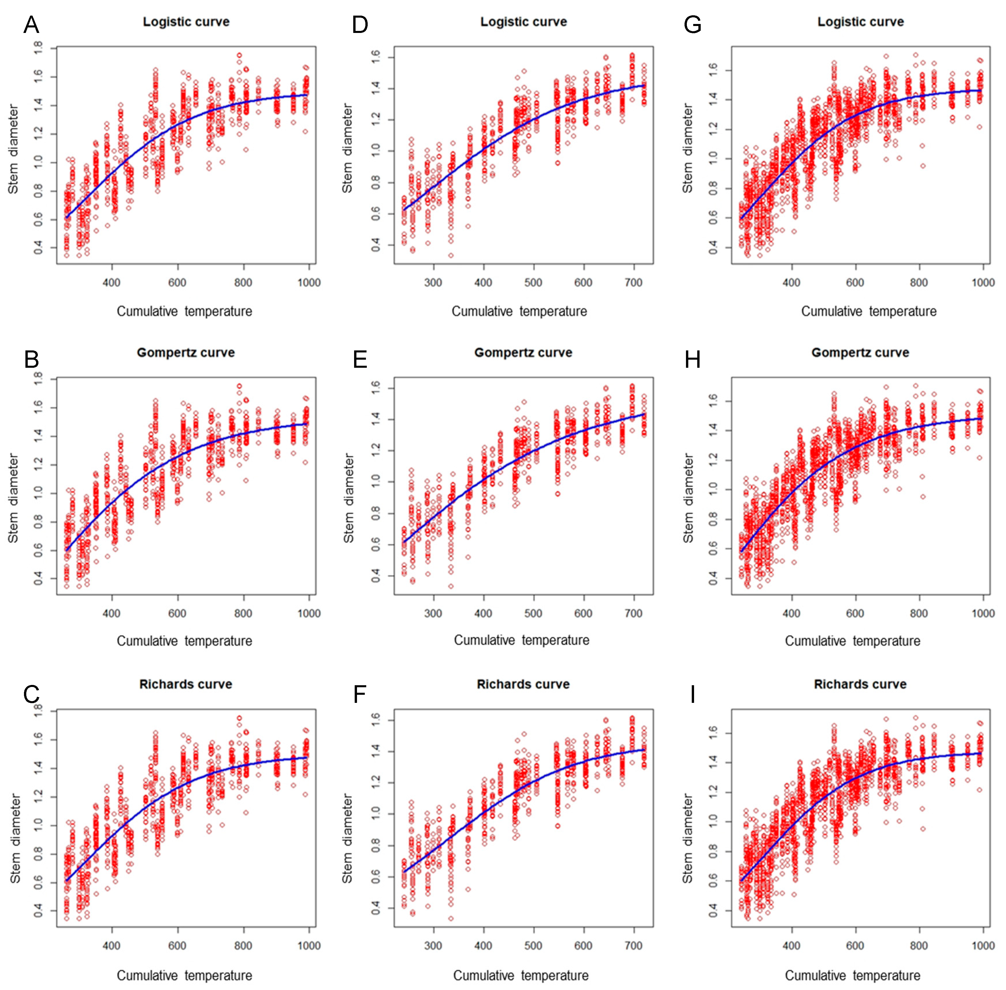
Figure 3 shows the plot of the eggplant stem diameter versus the cumulative temperature, with the fitted growth curves for the spring–summer, autumn–winter, and combined data sets. These plots suggest that the three nonlinear growth models were appropriate for the data. Additionally, the results presented in Table 3 indicate that the performance of the three nonlinear models did not differ markedly in the same growing season, with the difference being less than 0.01 among the R2 values for the three growth models. However, a difference in the performance of the models was noted among the different growing seasons. The autumn–winter model exhibited optimal performance (R2 = 0.85), followed by the global model (R2 = 0.83); the spring–summer model performed most poorly (R2 = 0.82; Table 3).
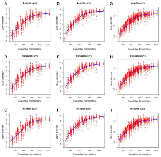
Figure 3.
Scatter plots of the eggplant stem diameter versus cumulative temperature, obtained using the logistic, Gompertz, and Richards models (blue curves) to fit the spring–summer, autumn–winter, and combined data sets. (A) Spring–summer Logistic model; (B) spring–summer Gompertz model; (C) spring–summer Richards model; (D) autumn–winter Logistic model; (E) autumn–winter Gompertz model; (F) autumn–winter Richards model; (G) global Logistic model; (H) global Gompertz model; (I) global Richards model.

Table 3.
R2, AIC, RMSE, and MAE of the eggplant rootstock training models used to fit the spring–summer, autumn–winter, and combined data sets.
Figure 4 illustrates that the fitting performance of the tomato scion model had a similar tendency to that of the eggplant rootstock model. In the same growing season, the performance of the three nonlinear models did not vary greatly, with differences in R2 values for the three growth models of less than 0.01. However, a significant difference across growing seasons was observed. Among the three growth models, the autumn–winter model performed optimally (R2 = 0.80), followed by the global model (R2 = 0.752); the spring–summer model was the worst performer (R2 = 0.746; Table 4). Regardless of whether the R2, AIC, RMSE, or MAE criterion was used, the fitting ability results were nearly identical (Table 3 and Table 4). Although these findings are slightly poorer than those of another study on sunn hemp [26], which reported model R2 values of 0.85–0.86 when using the Logistic and Gompertz nonlinear models to establish the relationship between the fresh stem mass of sunn hemp and the days after sowing, the growth models developed in the present study demonstrate acceptable fitting ability.
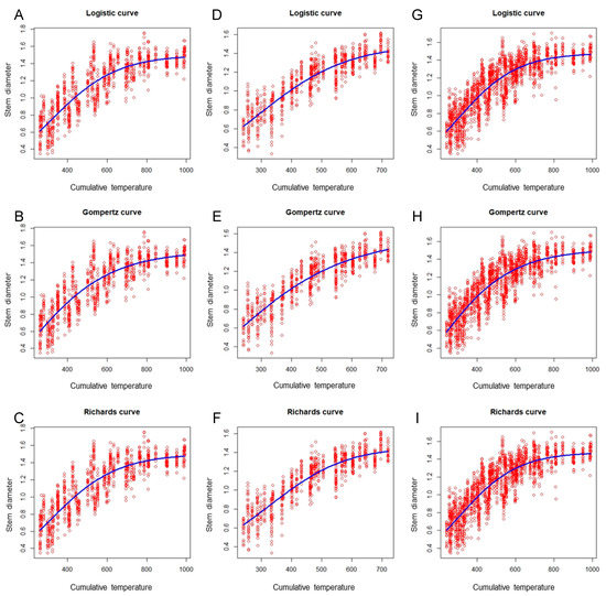
Figure 4.
Scatter plots of the tomato stem diameter versus cumulative temperature, obtained using the Logistic, Gompertz, and Richards models (blue curves) to fit the spring–summer, autumn–winter, and combined data sets. (A) Spring–summer Logistic model; (B) spring–summer Gompertz model; (C) spring–summer Richards model; (D) autumn–winter Logistic model; (E) autumn–winter Gompertz model; (F) autumn–winter Richards model; (G) global Logistic model; (H) global Gompertz model; (I) global Richards model.

Table 4.
R2, AIC, RMSE, and MAE of the tomato scion training models used to fit the spring–summer, autumn–winter, and combined data sets.
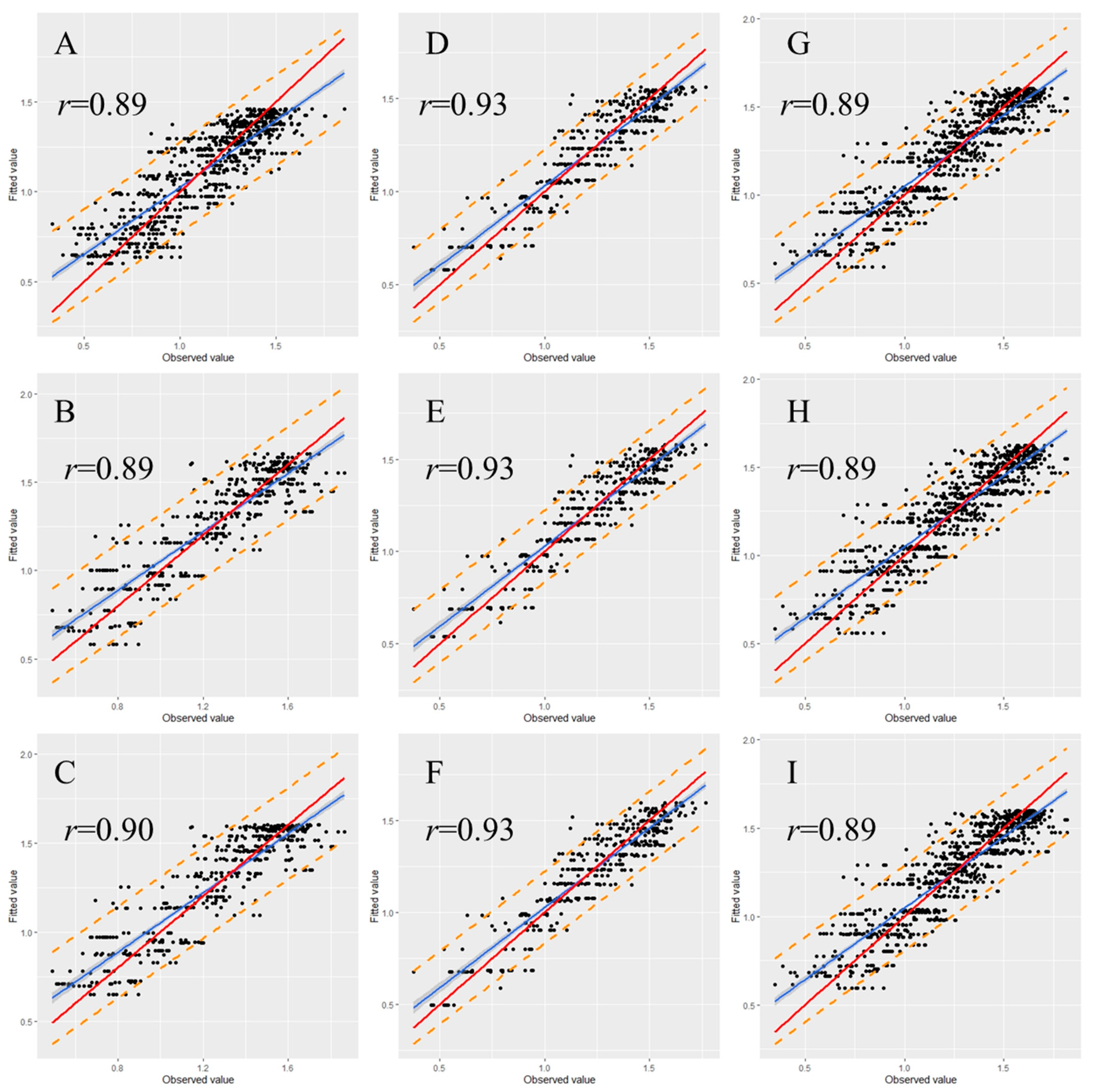
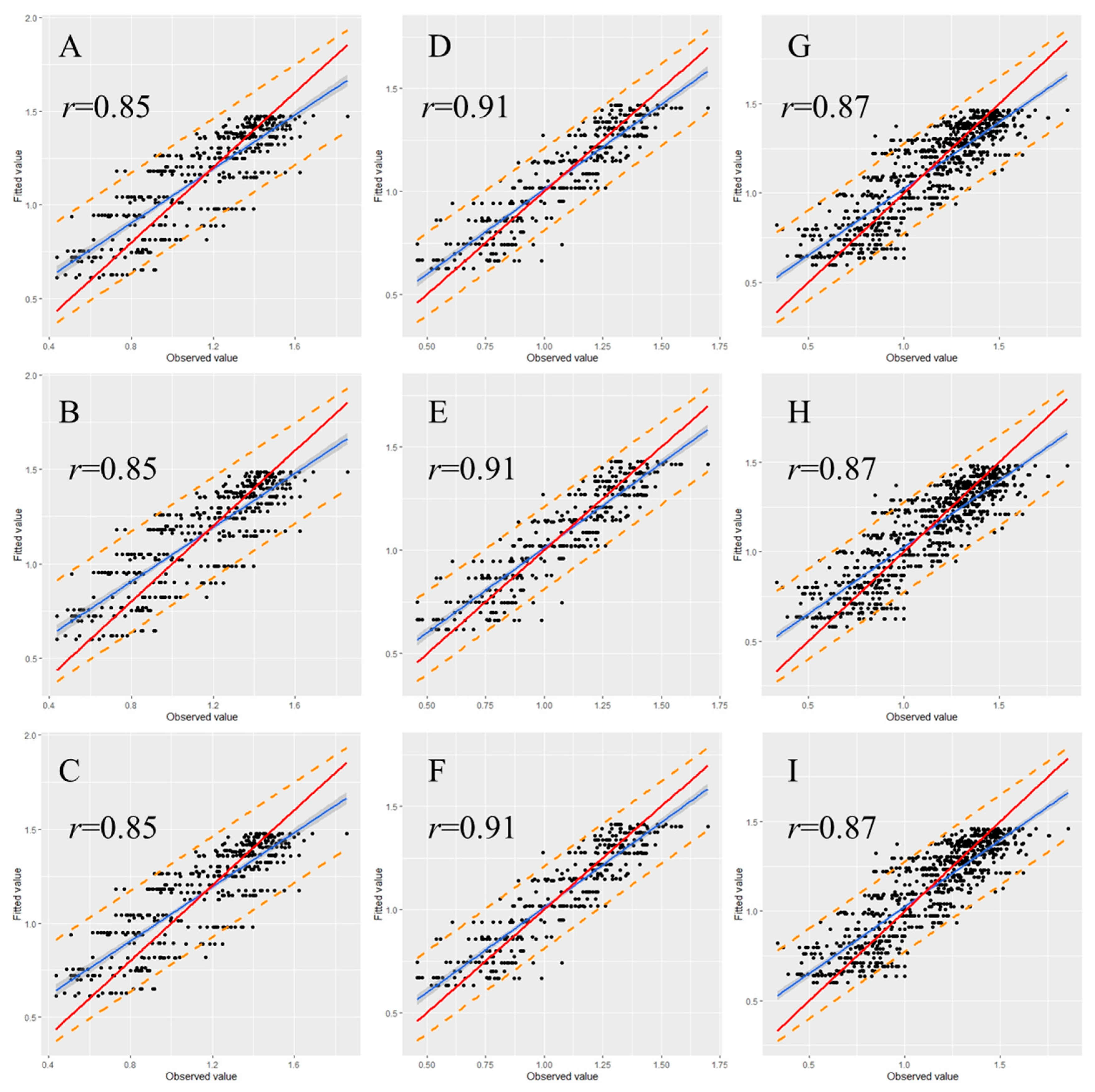
To examine the stability and rationality of the regression coefficients, validation is a necessary step in the model construction. Therefore, we randomly classified 30% of the data from each data set as a validation set. The graph illustrating the observed versus fitted values indicates that most of the data points were within the 95% prediction interval for each validated model (Figure 5 and Figure 6). Moreover, most of the observed values demonstrated no significant deviation from the straight line with a slope of 1, and the correlation coefficients (r) between observed and fitted values were all higher than 0.80 (Figure 5 and Figure 6), indicating that the fitted and observed values were close and the model had accurate predictive ability. Table 5 and Table 6 detail the performance of the eggplant and tomato validation models by using the spring–summer, autumn–winter, and combined data sets. The validation indicated that in the same growing season, the performance of the three nonlinear models did not greatly differ. Among the different-season models, the autumn–winter model had the highest performance. The R2 values for the eggplant and tomato models were 0.86 and 0.83, respectively. The global model registered the second-best results among the different-season models, with R2 values for the eggplant and tomato models of 0.80 and 0.75, respectively. The spring–summer model performed the worst, with R2 values for the eggplant and tomato models of 0.80 and 0.72, respectively (Table 5 and Table 6). Moreover, the validation results were noted to display the same tendency regardless of whether the R2, AIC, RMSE, or MAE criterion was used (Table 5 and Table 6).
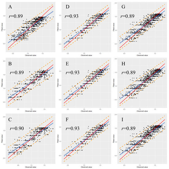
Figure 5.
Relationship between the fitted and observed values of the eggplant model. (A) Spring–summer Logistic model; (B) spring–summer Gompertz model; (C) spring–summer Richards model; (D) autumn–winter Logistic model; (E) autumn–winter Gompertz model; (F) autumn–winter Richards model; (G) global Logistic model; (H) global Gompertz model; (I) global Richards model. Prediction intervals are shown at a 95% level (dashed lines). The solid red lines represent the regression lines, and the dotted lines refer to the 1:1 lines.
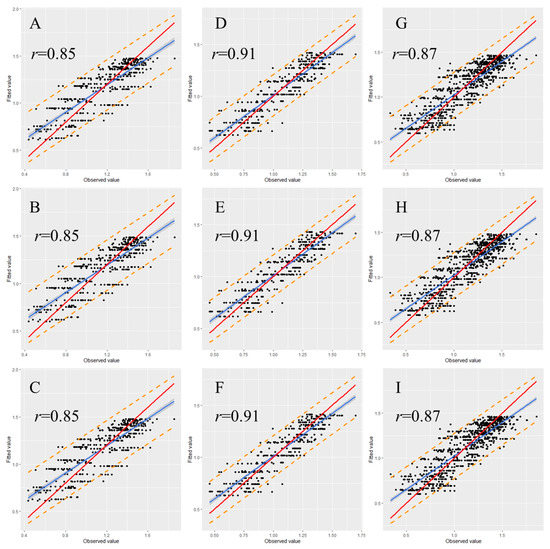
Figure 6.
Relationship between the fitted and observed values of the tomato model in validation. (A) Spring–summer Logistic model; (B) spring–summer Gompertz model; (C) spring–summer Richards model; (D) autumn–winter Logistic model; (E) autumn–winter Gompertz model; (F) autumn–winter Richards model; (G) global Logistic model; (H) global Gompertz model; (I) global Richards model. Prediction intervals are shown at a 95% level (dashed lines). The solid red lines represent the regression lines, and the dotted lines refer to the 1:1 lines.

Table 5.
R2, AIC, RMSE, and MAE of the eggplant validation models used to fit the spring–summer, autumn–winter, and combined data sets.

Table 6.
R2, AIC, RMSE, and MAE of the tomato validation models used to fit the spring–summer, autumn–winter, and combined data.
Notably, the spring–summer model of the tomato scion was outperformed by the two other models in both calibration and validation, with R2 being 0.72–0.746 (Table 4 and Table 6). We thus inferred that tomatoes are better adapted to autumn–winter production than to summer production in Taiwan. The summer environment restricts tomato growth. The Richards model, which allows for asymmetric growth, also performed suboptimally on all of the evaluation criteria except the AIC, for which it was only slightly outperformed by the Gompertz and Logistic models. Therefore, we conclude that introducing an additional parameter to explain asymmetric growth in the prediction of tomato (Rosada cultivar) and eggplant (EG203 cultivar) stem diameter at the seedling stage is unnecessary.
During the validation step, the fitted value of a model can be compared with the actual observed value to evaluate the predictive ability of the trained model [37]. Shah et al. [40] used weather-related variables to predict the probability of wheat head blight. Before establishing their Logistic regression model, 70% of all data were randomly selected as the training set for model construction, and the remaining 30% data were classified as the testing set used for the model validation. They identified the weather-related predictors through the model selection process to develop a relatively simple model. In the present study, the fitting and predictive capabilities of each model were generally favorable and the performance criteria for validation did not change significantly compared with the calibration, indicating that these models were not overfit. Hence, the models developed in this study should have high application potential.
3.3. Comparison of Model Parameters for Data from Different Growing Seasons
Table 7 displays the estimates and 95% confidence intervals for various eggplant parameters based on the three nonlinear growth models in different seasons. In the eggplant model, most parameter estimates varied significantly among the different seasons (Table 7). The Logistic model estimated parameter a as 1.6559 for the spring–summer data, which was outside of the 95% confidence interval (1.5486, 1.5917). Similarly, the model’s estimate of 1.5702 for the autumn–winter data was not within the 95% confidence interval (1.6275, 1.6842). Therefore, in different seasons, the models generated distinct parameter estimates despite having been developed using the same variables. These findings are consistent with those of previous studies [26,39], which demonstrated that the parameters estimated for sunn hemp were different when differing growth models were employed. Notably, the performance of growth models is affected by the growing season. However, no significant differences in parameter estimates for the tomato models were noted between the seasons; only the estimate of parameter c for the Logistic model was on the boundary (Table 8).

Table 7.
Estimates, SEs, and 95% confidence intervals of eggplant parameters based on the three nonlinear growth models in different seasons.

Table 8.
Estimates, SEs, and 95% confidence intervals of tomato parameters based on the three nonlinear growth models in different seasons.
In practice, a model that can fit various seasonal conditions is more widely applicable. Therefore, we combined the data from different seasons to test the generalizability of the models. Table 9 lists the eggplant and tomato parameter estimates and 95% confidence intervals obtained using three nonlinear growth models to fit the combined data. The parameter estimates of all global models were significantly different from those of the spring–summer and autumn–winter models for eggplant, except for parameter a in the Richards model (Table 7 and Table 9). Conversely, the Gompertz and Richards model parameter estimates for the global data did not significantly differ in relation to spring–summer and autumn–winter tomatoes (Table 8 and Table 9). Nevertheless, as mentioned in the previous section, the model fit and validation performance of the global model were inferior to those of the autumn–winter model (but superior to those of the spring–summer model (Table 3, Table 4, Table 5 and Table 6). Therefore, the various environmental conditions suggest that different growth models should be employed in different seasons to achieve optimal model validity.

Table 9.
Estimates, SEs, and 95% confidence intervals of eggplant and tomato parameters based on the three nonlinear growth models fitted to the combined data.
3.4. Estimation of a Suitable Grafting Standard by Using the Cumulative Daily Temperature
Three nonlinear growth models developed for different seasons were used to estimate the time required for eggplant rootstocks and tomato scions to reach the grafting standard (1.5–2.0 mm) given the cumulative daily temperature (Table 10). In spring–summer, the eggplant and tomato could be grafted when the cumulative temperature reached 578.2–724.1 and 567.4–789.2 °C, respectively; in autumn–winter, the eggplant and tomato could be grafted when the cumulative temperature reached 541.4–688.5 and 509.6–718.6 °C, respectively. The combined data for the various seasons suggested that the eggplant and tomato could be grafted when the cumulative temperature reached 558.8–702.8 and 540.3–770.6 °C, respectively. As detailed in Table 1, the average temperature recorded in each data set suggest that for grafting during spring–summer, eggplant and tomato require approximately 21–27 and 21–29 days, respectively. However, in the autumn–winter, the eggplant and tomato require nearly 23–29 and 22–31 days, respectively. In addition, the combined data indicate that eggplant grafting requires approximately 22–27 days, whereas tomato grafting requires 21–30 days (Table 10).

Table 10.
Summary of cumulative temperatures required to reach the seedling stem diameter standards of 1.5 and 2.0 mm for eggplant and tomato based on the spring–summer, autumn–winter, and combined data sets and calculated using the three nonlinear growth models.
In summary, if the stem diameter of 1.5 mm is selected as the grafting standard, the growing time of eggplant is nearly 1 day longer than that of tomato, except during spring–summer. By contrast, the required eggplant growth time is 1–2 days shorter than that of tomato when 2.0 mm is designated as the necessary stem diameter for grafting (Table 10). However, Norday et al. [5] considered seedling stem diameter as a dependent variable and employed multiple linear regression analysis on two independent variables (i.e., the number of days after sowing and the temperature), discovering that the eggplant rootstocks required more growth time than the tomato scions to reach the 1.6 mm stem diameter they deemed suitable for grafting based on personal experience. The eggplant rootstock growth time was approximately 2 weeks longer than that of the tomato scion. This is not entirely consistent our results; the difference could have resulted from the different experimental materials, environmental conditions, or statistical models.
Stem diameter is the most crucial indicator in evaluation of grafting timing because the stem diameters of the rootstock and scion seedlings must not only be within a certain range but also be similar at the time of grafting [41,42,43]. Several studies have suggested that the stem diameter of the rootstock and scion being similar during grafting increases the grafting success rate [20,22,23]. Other suitable stem diameters of eggplant rootstock and tomato scion (e.g., 2.0 mm for tomato scion and 2.5 mm for eggplant rootstock) are planned topics of our further studies in Taiwan. In addition, during the growth process, crops are highly susceptible to environmental conditions, which affect their growth rates. Therefore, to more effectively control error variation and improve a model’s interpretation and predictive ability, the amount of data gathered during the data collection stage can be increased or additional independent model variables (e.g., varieties and environmental factors) can be considered. Jones et al. [44] estimated several physiological parameters of tomato under various environmental conditions, asserting that estimating the parameters based on specific cultivation conditions and crop varieties necessitates the use of an established growth model. Yuan and Bland [45] modeled the weights of the stems, leaves, and tubers of potatoes (Solanum tuberosum) by using two independent variables (i.e., temperature and photosynthetically active radiation), reporting that the growth and development of potatoes were greatly influenced by the weather and field management procedure in response to local seasonal weather differences. The models established in the current study were constructed using only the data of a single region. We plan in our future works to acquire data from other regions to improve our model’s ability to predict the stem diameter of eggplant rootstocks and tomato scions.
4. Conclusions
In the present study, we collected seedling growth data for a total of 3 years (six growing seasons) in Taiwan and established growth models by using three sigmoid growth functions: the Gompertz, Logistic, and Richards models. The nonlinear growth models established in this study can accurately predict the growth of the stem diameter of eggplant and tomato. It is unnecessary to introduce an additional parameter to explain asymmetric growth in the prediction of tomato (Rosada cultivar) and eggplant (EG203 cultivar) stem diameter at the seedling stage. When these models are used to predict the growth of seedlings, the cumulative temperature predictions through local weather forecasts or historical weather data can be used to adjust the planned sowing and grafting times of eggplant and tomato. Similarly, nurseries can plant different batches of seedlings at the optimal time and arrange the schedule of grafting operations in advance to improve grafting efficiency. Taking Taiwan environmental conditions as an example, we can predict that when grafting during spring–summer, eggplant and tomato, it will require approximately 21–27 and 21–29 days to reach cumulative temperature; while in the autumn–winter, it will take nearly 23–29 and 22–31 days, respectively. Basically, tomato must be sown 1–2 days earlier than eggplant. With this information, the planting date can be scheduled in advance according to the market demands.
Supplementary Materials
The following are available online at https://www.mdpi.com/article/10.3390/horticulturae7120537/s1, Table S1: Descriptive statistics of the environmental parameters of each data set used in this study (information presented separately by year). Figure S1: Residual plots of eggplant stem diameter (untransformed) by using spring–summer, autumn–winter, and combined data with the Logistic, Gompertz, and Richards growth models. Figure S2: Residual plots of tomato stem diameter (untransformed) by using spring–summer, autumn–winter, and combined data with the Logistic, Gompertz, and Richards growth models.
Author Contributions
Conceptualization, B.-J.K., C.-Y.H. and S.-L.F.; data curation, C.-Y.H., S.-L.F., Y.-F.W. and Y.-C.C.; formal analysis, C.-Y.H. and S.-L.F.; funding acquisition, B.-J.K.; investigation, Y.-F.W. and Y.-C.C.; methodology, B.-J.K., C.-Y.H. and S.-L.F.; writing—original draft, B.-J.K., C.-Y.H. and S.-L.F.; writing—review and editing, B.-J.K. All authors have read and agreed to the published version of the manuscript.
Funding
This research was funded by Agricultural and Food Agency, Council of Agriculture under Grant Number 109AS-11.2.2-FD-Z1. The Ministry of Education (MOE) provided partial funding in the form of a grant awarded to B.-J.K., through the Innovation and Development Center of Sustainable Agriculture, from The Featured Areas Research Center Program, within the framework of the Higher Education Sprout Project by the MOE in Taiwan.
Data Availability Statement
Not applicable.
Conflicts of Interest
The authors declare no conflict of interest.
References
- García-Alonso, F.J.; Bravo, S.; Casas, J.; Pérez-Conesa, D.; Jacob, K.; Periago, M.J. Changes in antioxidant compounds during the shelf life of commercial tomato juices in different packaging materials. J. Agric. Food Chem. 2009, 57, 6815–6822. [Google Scholar] [CrossRef]
- Manickam, R.; Chen, J.R.; Sotelo-Cardona, P.; Kenyon, L.; Srinivasan, R. Evaluation of different bacterial wilt resistant eggplant rootstocks for grafting tomato. Plants 2021, 10, 75. [Google Scholar] [CrossRef] [PubMed]
- Perveen, R.; Suleria, H.A.R.; Anjum, F.M.; Butt, M.S.; Pasha, I.; Ahmad, S. Tomato (Solanum lycopersicum) carotenoids and lycopenes chemistry; metabolism, absorption, nutrition, and allied health claims—A comprehensive review. Crit. Rev. Food Sci. Nutr. 2015, 55, 919–929. [Google Scholar] [CrossRef]
- Rosales, M.A.; Cervilla, L.M.; Sánchez-Rodríguez, E.; Rubio-Wilhelmi, M.; Blasco, B.; Ríos, J.J.; Soriano, T.; Castilla, N.; Romero, L.; Ruiz, J.M. The effect of environmental conditions on nutritional quality of cherry tomato fruits: Evaluation of two experimental Mediterranean greenhouses. J. Sci. Food Agric. 2011, 91, 152–162. [Google Scholar] [CrossRef] [PubMed]
- Norday, T.; Shem, E.; Huat, J. Impacts of temperature and rootstocks on tomato grafting success rates. HortScience 2020, 55, 136–140. [Google Scholar] [CrossRef]
- Kubota, C.; McClure, M.A.; Kokalis-Burelle, N.; Bausher, M.G.; Rosskopf, E.N. Vegetable grafting: History, use, and current technology status in North America. HortScience 2008, 43, 1664–1669. [Google Scholar] [CrossRef]
- Lee, J.M.; Kubota, C.; Tsao, S.J.; Bie, Z.; Echevarria, P.H.; Morra, L.; Oda, M. Current status of vegetable grafting: Diffusion, grafting techniques, automation. Scientia Hort. 2010, 127, 93–105. [Google Scholar] [CrossRef]
- Lee, J.M. Cultivation of grafted vegetables. I. Current status, grafting methods, and benefits. HortScience 1994, 29, 235–239. [Google Scholar] [CrossRef]
- Lee, J.M.; Oda, M. Grafting of herbaceous vegetable and ornamental crops. Hortic. Rev. 2003, 28, 61–124. [Google Scholar]
- Morra, L. Potential and limits of grafting in horticulture. Inf. Agrar. 1998, 54, 39–42. [Google Scholar]
- Xu, Q.; Guo, S.R.; Li, H.; Du, N.S.; Shu, S.; Sun, J. Physiological aspects of compatibility and incompatibility in grafted cucumber seedlings. J. Am. Soc. Hort. Sci. 2015, 140, 299–307. [Google Scholar] [CrossRef]
- Kumar, P.; Rouphael, Y.; Cardarelli, M.; Colla, G. Vegetable grafting as a tool to improve drought resistance and water use efficiency. Front. Plant Sci. 2017, 8, 1130. [Google Scholar] [CrossRef]
- Rouphael, Y.; Cardarelli, M.; Rea, E.; Colla, G. Improving melon and cucumber photosynthetic activity, mineral composition, and growth performance under salinity stress by grafting onto Cucurbita hybrid rootstocks. Photosynthetica 2012, 50, 180–188. [Google Scholar] [CrossRef]
- Savvas, D.; Colla, G.; Rouphael, Y.; Schwarz, D. Amelioration of heavy metal and nutrient stress in fruit vegetables by grafting. Sci. Hort. 2010, 127, 156–161. [Google Scholar] [CrossRef]
- Schwarz, D.; Rouphael, Y.; Colla, G.; Venema, J.H. Grafting as a tool to improve tolerance of vegetables to abiotic stresses: Thermal stress, water stress and organic pollutants. Sci. Hort. 2010, 127, 162–171. [Google Scholar] [CrossRef]
- Venema, J.H.; Dijk, B.E.; Bax, J.M.; van Hasselt, P.R.; Elzenga, J.T.M. Grafting tomato (Solanum lycopersicum) onto the rootstock of a high-altitude accession of Solanum habrochaites improves suboptimal-temperature tolerance. Environ. Expt. Bot. 2008, 63, 359–367. [Google Scholar] [CrossRef]
- Morikawa, C.K. Reducing cadmium accumulation in fresh pepper fruits by grafting. Hort. J. 2017, 86, 45–51. [Google Scholar] [CrossRef]
- Xie, Y.D.; Tan, H.Q.; Sun, G.C.; Li, H.X.; Liang, D.; Xia, H.; Wang, X.; Liao, M.A.; Deng, H.H.; Wang, J.; et al. Grafting alleviates cadmium toxicity and reduces its absorption by tomato. Soil Sci. Plant Nutr. 2020, 20, 2222–2229. [Google Scholar] [CrossRef]
- Naik, S.A.T.S.; Hongal, S.; Harshavardhan, M.; Chandan, K.; Kumar, A.J.S.; Ashok; Kyriacou, M.C.; Rouphael, Y.; Kumar, P. Productive characteristics and fruit quality traits of cherry tomato hybrids as modulated by grafting on different Solanum spp. rootstocks under Ralstonia solanacearum infested greenhouse soil. Agronomy 2021, 11, 1311. [Google Scholar] [CrossRef]
- Singh, H.; Kumar, P.; Chaudhari, S.; Edelstein, M. Tomato grafting: A global perspective. HortScience 2017, 52, 1328–1336. [Google Scholar] [CrossRef]
- Singh, H.; Kumar, P.; Kumar, A.; Kyriacou, M.C.; Colla, G.; Rouphael, Y. Grafting tomato as a tool to improve salt tolerance. Agronomy 2020, 10, 263. [Google Scholar] [CrossRef]
- Bumgarner, N.R.; Kleinhenz, M.D. Grafting guide—A pictorial guide to the cleft and splice graft methods. Ohio Agr. Res. Dev. Ctr. Bul. 2014, 950. [Google Scholar]
- Rivard, C.L.; Louws, F.J. Grafting for disease resistance in heirloom tomatoes. Ext. Folder NC Agric. Ext. Serv. 2006, 8. [Google Scholar]
- Guzmán, G.; Morales, M.; Pukkala, T.; de-Miguel, S. A model for predicting the growth of Eucalyptus globulus seedling stands in Bolivia. For. Syst. 2012, 21, 205–209. [Google Scholar] [CrossRef][Green Version]
- Streck, N.; Bosco, L.C.; Lucas, D.D.P.; Lago, I. Modelagem da emissão de folhas em arroz. Pesqui. Agropecu. Bras. 2008, 43, 559–567. [Google Scholar] [CrossRef]
- Bem, C.M.; Cargnelutti Filho, A.; Facco, G.; Schabarum, D.E.; Silveira, D.L.; Simões, F.M.; Uliana, D.B. Growth models for morphological traits of sunn hemp. Semin. Cienc. Agrar. 2017, 38, 2933–2944. [Google Scholar] [CrossRef]
- Gomes, A.C.S.; Robaina, A.D.; Peiter, M.X.; Soares, F.C.; Parizi, A.R.C. Modelo para estimativa da produtividade para a cultura da soja. Cienc. Rural 2014, 44, 43–49. [Google Scholar] [CrossRef]
- Archontoulis, S.A.; Miguez, F.E. Nonlinear regression models and applications in agricultural research. Agron. J. 2015, 107, 786–798. [Google Scholar] [CrossRef]
- Gan, Y.; Stobbe, E.H.; Njue, C. Evaluation of selected nonlinear regression models in quantifying seedling emergence rate of spring wheat. Crop Sci. 1996, 36, 165–168. [Google Scholar] [CrossRef]
- Miguez, F.E.; Zhu, X.; Humphries, S.; Bollero, G.A.; Long, S.P. A semimechanistic model predicting growth and production of the bioenergy crop Miscanthus × giganteus: Description, parameterization and validation. Glob. Change Biol. Bioenergy 2009, 1, 282–296. [Google Scholar] [CrossRef]
- Gompertz, B. On the nature of the function expressive of the law of human mortality, and on a new mode of determining the value of life contingencies. Philos. Trans. R. Soc. 1825, 115, 513–585. [Google Scholar]
- Verhulst, P.F. A note on population growth. Corresp. Math. Phys. 1838, 10, 113–121. [Google Scholar]
- Lucio, A.D.; Nunes, L.F.; Rego, F. Nonlinear models to describe production of fruit in Cucurbita pepo and Capiscum annuum. Sci. Hortic. 2015, 193, 286–293. [Google Scholar] [CrossRef]
- Gonzaga, T.W.C.; Mata, M.E.; Silva, H.; Duarte, M.E. Crioconservação de sementes de aroeira (Astronium urundeuva Engl.), e baraúna (Schinopsis brasiliensis Engl.). Rev. Bras. Prod. Agroind. 2003, 5, 145–154. [Google Scholar] [CrossRef]
- Martins Filho, S.; Silva, F.F.; Carneiro, A.P.; Muniz, J.A. Abordagem bayesiana das curvas de crescimento de duas cultivares de feijoeiro. Cienc. Rural 2008, 38, 1516–1521. [Google Scholar] [CrossRef]
- Richards, F.J. A flexible growth function for empirical use. J. Exp. Bot. 1959, 10, 290–300. [Google Scholar] [CrossRef]
- Kutner, M.H.; Nachtsheim, C.J.; Neter, J.; Li, W. Applied Linear Statistical Models, 5th ed.; McGraw-Hill: New York, NY, USA, 2004. [Google Scholar]
- Filliben, J.J. The probability plot correlation coefficient test for normality. Technometrics 1975, 17, 111–117. [Google Scholar] [CrossRef]
- Bem, C.M.; Cargnelutti Filho, A.; Chaves, G.G.; Kleinpaul, J.A.; Lavezo, A. Gompertz and Logistic models to the productive traits of sunn hemp. J. Agric. Sci. 2018, 10, 225–238. [Google Scholar] [CrossRef]
- Shah, D.A.; Molineros, J.E.; Paul, P.A.; Willyerd, K.T.; Madden, L.V.; De Wolf, E.D. Predicting Fusarium head blight epidemics with weather-driven pre-and post-anthesis Logistic regression models. Phytopathology 2013, 103, 906–919. [Google Scholar] [CrossRef]
- Hu, B.; Bennett, M.A.; Kleinhenz, M.D. A new method to estimate vegetable seedling vigor, piloted with tomato, for use in grafting and other contexts. HortTechnology 2016, 26, 767–775. [Google Scholar] [CrossRef]
- Oda, M.; Tsuji, K.; Sasaki, H. Effect of hypocotyl morphology on survival rate and growth of cucumber seedlings grafted on Cucurbita spp. Jpn. Agr. Res. Qrtly. 1993, 26, 259–263. [Google Scholar]
- Yetisxir, H.; Sari, N. Effect of hypocotyl morphology on survival rate and growth of watermelon seedlings grafted on rootstocks with different emergence performance at various temperatures. Turk. J. Agr. For. 2004, 28, 231–237. [Google Scholar]
- Jones, J.W.; Kenig, A.; Vallejos, C.E. Reduced state-variable tomato growth model. Trans. ASAE 1999, 42, 255–265. [Google Scholar] [CrossRef]
- Yuan, F.M.; Bland, W.L. Comparison of light and temperature based index models for potato (Solanum tuberosum L.) growth and development. Am. J. Potato. Res. 2005, 82, 345–352. [Google Scholar] [CrossRef]
Publisher’s Note: MDPI stays neutral with regard to jurisdictional claims in published maps and institutional affiliations. |
© 2021 by the authors. Licensee MDPI, Basel, Switzerland. This article is an open access article distributed under the terms and conditions of the Creative Commons Attribution (CC BY) license (https://creativecommons.org/licenses/by/4.0/).

