Article

Using a Hybrid Neural Network Model DCNN–LSTM for Image-Based Nitrogen Nutrition Diagnosis in Muskmelon

School of Agriculture and Biology, Shanghai Jiao Tong University, Shanghai 200240, China
*
Author to whom correspondence should be addressed.
Horticulturae 2021, 7(11), 489; https://doi.org/10.3390/horticulturae7110489
Submission received: 26 October 2021 / Revised: 8 November 2021 / Accepted: 8 November 2021 / Published: 12 November 2021

Abstract

:
In precision agriculture, the nitrogen level is significantly important for establishing phenotype, quality and yield of crops. It cannot be achieved in the future without appropriate nitrogen fertilizer application. Moreover, a convenient and real-time advance technology for nitrogen nutrition diagnosis of crops is a prerequisite for an efficient and reasonable nitrogen-fertilizer management system. With the development of research on plant phenotype and artificial intelligence technology in agriculture, deep learning has demonstrated a great potential in agriculture for recognizing nondestructive nitrogen nutrition diagnosis in plants by automation and high throughput at a low cost. To build a nitrogen nutrient-diagnosis model, muskmelons were cultivated under different nitrogen levels in a greenhouse. The digital images of canopy leaves and the environmental factors (light and temperature) during the growth period of muskmelons were tracked and analyzed. The nitrogen concentrations of the plants were measured, we successfully constructed and trained machine-learning- and deep-learning models based on the traditional backpropagation neural network (BPNN), the emerging convolution neural network (CNN), the deep convolution neural network (DCNN) and the long short-term memory (LSTM) for the nitrogen nutrition diagnosis of muskmelon. The adjusted determination coefficient (R2) and mean square error (MSE) between the predicted values and measured values of nitrogen concentration were adopted to evaluate the models’ accuracy. The values were R2 = 0.567 and MSE = 0.429 for BPNN model; R2 = 0.376 and MSE = 0.628 for CNN model; R2 = 0.686 and MSE = 0.355 for deep convolution neural network (DCNN) model; and R2 = 0.904 and MSE = 0.123 for the hybrid model DCNN–LSTM. Therefore, DCNN–LSTM shows the highest accuracy in predicting the nitrogen content of muskmelon. Our findings highlight a base for achieving a convenient, precise and intelligent diagnosis of nitrogen nutrition in muskmelon.

1. Introduction

The netted muskmelon (Cucumis melo L. var. etiquettes Naud.) is a delicious and nutritious fruit. It is widespread and grown worldwide. Nitrogen is one of the critical environmental factors that affects the growth process of muskmelon. Both the external phenotype and internal activity are significantly affected by nitrogen [1,2,3]. The appropriate nitrogen levels are helpful for the accumulation of nitrogen and fruit biomass production in crops [4,5]. However, farmers often overuse nitrogen in muskmelon, and this reduces the quality and yield of muskmelon fruit. At the same time, the overuse of nitrogen causes serious environmental problems, such as contamination of water resources, nitrogen leaching losses and emission of greenhouse gases [6,7]. Therefore, an efficient and real-time nitrogen nutrition diagnosis technology is necessary for achieving the goal of rational nitrogen application in crops.
Traditionally, crop nitrogen nutrition status is artificially judged by plant phenotypical traits or determined with the chemical analysis method. However, the plant-image-based artificial judgment is empirical, and the chemical analysis method is destructive for the plants. After all, phenotypical traits of crops can help to guide real-time fertilizer applications to the plants in greenhouses and fields [8]. At present, image-based machine vision techniques have been adopted for plant nutrition diagnosis in agriculture sector. These techniques can detect automatically or semi-automatically the slight changes in leaves’ reflection characteristics to visible light due to variation in different nutrition levels of the plants [3]. Machine learning techniques could be considered effective processes which are used to analyze the big data and give efficient results with outstanding performance in many fields, such as artificial neural network, decision tree, support vector machine (SVM), etc. Therefore, combining machine vision technique with machine learning is an ideal choice for realizing the nondestructive diagnosis of plants’ nitrogen nutrition. Non-destructive testing technology is more efficient and accurate than traditional manual measurement methods. This technology is cheaper and requires less time than hyperspectral [9,10,11] and chlorophyll fluorescence [10,12]. It has been used in many agricultural fields, such as biomass accumulation through image analysis [13], crop coefficient [14], abiotic stresses [15,16] and nutritional diagnosis [3,17,18].
Deep learning is considered to be a promising and advanced subset of machine learning. It has emerged as a technique to process and analyze large and complex datasets. Now, it has been used in image-based plant phenotyping [19], plant species and pest identification [20,21,22,23,24], yield prediction [25,26,27] and protein and gene identification [28,29]. Concerning the prediction accuracy, deep learning methods give direct information as inputs of images’ data into the deep neural networks. It is helpful to avoid artificial image processing steps in data processing to filter out the redundant information of the images and reduction in dimensions [30]. The use of deep learning in agriculture to perform nitrogen nutrition diagnosis for crops, such as maize [31], rape [32] and masson pine [33], and showed remarkable potential in agriculture. This technique promptly predicts nitrogen status before appearance of nitrogen deficiency symptoms in plants and guides real-time nitrogen application in plants. It has a huge significance for improving crop quality and yield. Many studies used canopy leaf reflectance spectrum information for nitrogen nutrition diagnosis through deep learning [34,35], but limited data have been found for phenotypes and nitrogen nutrition diagnosis of muskmelon through image-based plant phenotyping in light and deep learning.
In deep learning, a convolution neural network (CNN) is a class of feed-forward neural networks in which sets of images are filtered through convolution and other pooling layers for feature extraction of images. Convolutional images or feature maps are obtained by repeating convolutional and other pooling layers for getting labeled estimated class in the model network as an output. In a training dataset, handcrafted features are used in traditional machine learning techniques while CNN is not this way [36]. In CNN, images are used to filter parameters by optimizing the weights in the hidden layers to generate the parameters of the features that are suitable to solve the classification problems. In principle, backpropagation is used to optimize the parameters in the model network [37], and classification errors are minimized by using gradient descent approaches [38]. By extracting the feature parameters as an interpretable form in CNN model confirms its reliability. In the training dataset, model authenticity and validation can be checked by the human interference.
In deep learning, CNN is developed for few hidden layers to extract the features from images, while, in recent years, neural networks with more layers have emerged and are called deep convolutional neural network (DCNN). Deep CNN has the same extraction features and performance as CNN, but it includes hidden layers and larger space for extraction features from images. In DCNN, the number of hidden layers greater than in CNN. In deep CNN, extraction features are performed automatically from the image processing, while, in CNN, extraction features from the image processing are performed by human interference. The extraction features are distributed across the layers by fine-tuning in an optimal way for the learning process in DCNN. It is not easy to adequately determine the most important extraction features in deep learning for large and/or complex datasets for human being. For that reason, we noticed a significant progress and achievement in accurate determination of different models in different fields when compared with other machine learning and/or deep learning methods [39]. Lin et al. [40] used the CNN semantic segmentation method for the identification of powdery mildew in cucumber. The model identified the powdery mildew by intersection over union (72.11%), dice accuracy (83.45%) and average pixel accuracy (96.08%) in the CNN model. CNN is mostly used for visual plant disease related problems in plants, but there are rare works in the literature on the comparison of CNN and DCNN in plant nutrition.
Deep CNN is mostly used for spatial data; deep recurrent neural network is built for sequential data modeling, such as time series [41,42]. It used widely in speech recognition, machine translation, emotion analysis and picture description. The input volume can be put as a series of text, speech, time, etc., that depends on previous elements. The time steps at the same state (input, output and hidden conditions) share one weight matrix, which greatly reduces the number of parameters to be learned in the model. DCNN model used to identify the nutrients deficiencies (nitrogen (N), potassium (K) and calcium (Ca)) in tomato leaves and fruiting phase accurately [43]. DCNN with the AlexNet model showed the highest accuracy rate of a model (92.1%) on the five different types of vegetables’ images-based dataset (mushrooms, pumpkin, broccoli, cucumber and cauliflower) [44] as compared to backpropagation neural network (BPNN) (78%) and support vector machines (SVM) classifier (80.5%). The DCNN model was used in cucumber to identify the cucumber diseases with the average pixel accuracy (93.4%) [24].
However, standard deep RNN may not be quite suitable for long-range order or memories in time series modeling. In such cases, long short-term memory (LSTM) has been reported as an effective and popular method in time series. Long short-term memory (LSTM) is a variant of RNN that can learn long-term dependence and is the most widely used. Compared with the traditional RNN, LSTM introduces controllable self-cycling, which is more suitable for processing and predicting important events with relatively long intervals or delays in time series. The network solves problems such as gradient disappearance and gradient explosion caused by time backpropagation during training [45]. Jiang et al. [46] used LSTM to predict the corn yield by using soil and weather data and described promising results. Wheat forecast production is accurately predicted by using LSTM model [47]. Plant growth variation and forecast yield production in tomato and Ficus benjamina stem growth by LSTM showed promising results in the controlled environments [48]. LSTM showed a great ability to disclose phenological properties, while DCNN has a great ability to extract more spatial features [49]. However, little attention has been directed to use the DCNN and LSTM for nitrogen nutrition in muskmelon.
This study aimed to predict the nitrogen content of greenhouse netted muskmelon accurately in real-time and guide the decision-making of nitrogen application of muskmelon in the greenhouse by using machine-learning or deep-learning approaches. Based on leaf images and measured nitrogen values, nitrogen nutrition diagnosis models were established and optimized by using machine learning or deep learning approaches. Nitrogen nutrition diagnosis by different deep learning models, step by step, is shown in Figure 1.

2. Materials and Methods

A thick-skinned netted muskmelon variety, Wanglu, was used as the material in this study. This experiment was carried out in a Venlo glass greenhouse (31°11′ N, 121°36′ E), C-2 block at Shanghai Jiao Tong University, from March 2018 to June 2018.
The seedlings of muskmelon Wanglu variety were grown in the seedling tray and then transplanted into pots containing a substrate “vermiculite and peat moss, 1:1 v/v” at the three-leaves stage. Each pot contained two plants (Figure 2). The pH of growing substrate of muskmelon was 6.77 and contained the following nutrients: available nitrogen at 332 mg/kg, available phosphorus at 124 mg/kg and available potassium at 118 mg/kg. Two weeks after transplanting, the muskmelon plants were treated with four different nitrogen applications with three replications. Different treatments of nitrogen were as follows: T1, 2.7 g nitrogen/pot; T2, 5.4 g nitrogen/pot; T3, 8.1 g nitrogen/pot; and T4, 10.8 g nitrogen/pot. The amount of phosphorus and potassium added per pot was 5.2 and 9.0 g, respectively, in all the pots. The sources of N, P and K fertilizers were calcium nitrate, potassium nitrate, magnesium nitrate and potassium dihydrogen phosphate. The total N fertilizer was applied at six growing stages of muskmelon, namely pre-planting (10%), seedling stage (5%), vine elongation stage (10%), initial fruit stage (35%), fruit expanding stage (35%) and mature stage (5%). All other nitrogen fertilizer applications were applied with drip irrigation, for except pre-planting (10%).
In this experiment, three fruiting vines kept in the beginning at the 10th–16th fruiting nodes, and later only one elegant-shaped big fruit and single main vine were kept, and we removed all redundant side vines at the 20–22 leaves stage. Hand-pollination was performed in time to ensure the fruit set.
The flowchart of this study is described in Figure 3. Four different treatments of nitrogen were applied to muskmelon and after harvesting, determined the nitrogen concentration in muskmelon. For this purpose, we collected the digital images from four fully expanded apical leaves for the whole growth period of muskmelon and measured the nitrogen concentration of muskmelon. Based on leaf images and measured nitrogen values, nitrogen nutrition diagnosis models were established and optimized by using machine learning or deep learning approaches.
In the machine learning-based nitrogen nutrition diagnosis models, plantCV, an open-source software for image analysis, was utilized to extract phenotypical features from the plants’ images. Furthermore, ANOVA and principal component analysis (PCA) were performed to analyze feature extraction parameters and reduced the dimensions. After that, three principal components were chosen. Dataset 1 was obtained by combining three principal components and nitrogen concentration data, and then it was randomly divided into a training subset (80%) and test subset (20%).
A backpropagation neural network (BPNN) model was built and trained by dataset 1. BPNN is not a two-layer network but with only 1 hidden layer. In BPNN, we used Empirical Formula (1) to calculate the hidden neurons. After testing, we set the number of hidden neurons at 12. In the BPNN model, we set 50 epochs, 100 epochs, 200 epochs, etc. In addition, we found a decline in accuracy after training 100 epochs. Therefore, we stopped training.
We also established a nitrogen nutrition diagnosis model based on deep learning approaches (Figure 3). First, the original dataset of images was processed through data augmentation, normalization, annotation, stitching, etc. Secondly, Dataset 2 was created by combining the processed dataset of images with nitrogen concentrations data, and then it was randomly divided into a training subset (80%), validation subset (10%) and test subset (10%).
Thirdly, convolutional neural network (CNN) and deep convolutional neural network (DCNN) models were built and trained by Dataset 2. Dataset 3 was covered by combing the processed dataset of images with nitrogen-concentration data and the dataset of meteorological factors. It was also randomly divided into a training subset (80%), validation subset (10%) and test subset (10%). A hybrid model based on DCNN–LSTM was finally built and evaluated by Dataset 3 as input data.
At last, the precision accuracy of all the models was compared to choose the best one among them.

3. Data Collection

3.1. Measurement of Nitrogen Concentration in Plants

For nitrogen measurement, plant samples were collected total of thirteen times throughout the experimental period at different growth stages. The first sampling was after the 5th day of nitrogen application at the seedling stage (5%) in pots. Each time, one plant from each pot was collected, and total 156 plant samples were collected from seedling stage to fruit maturity stage, with the interval of one week. After the removal of the abovementioned ground parts, digital images of leaves were collected. Only the four fully expanded leaves at the apical part of the plants were used for digital images analysis. Nitrogen concentration in plants was measured by mixing of all plants leaves. The plant leaves were used for nitrogen measurement by initially subjected to 30-min enzyme deactivation treatment at 105 °C, followed by drying at 80 °C to a constant weight, and finally ground into pieces of 100 mesh sieves. Nitrogen concentration was ultimately determined by elemental analysis isotope mass spectrometer Vario EL III/Isoprime element analyzer (Hanau, Germany) [50].

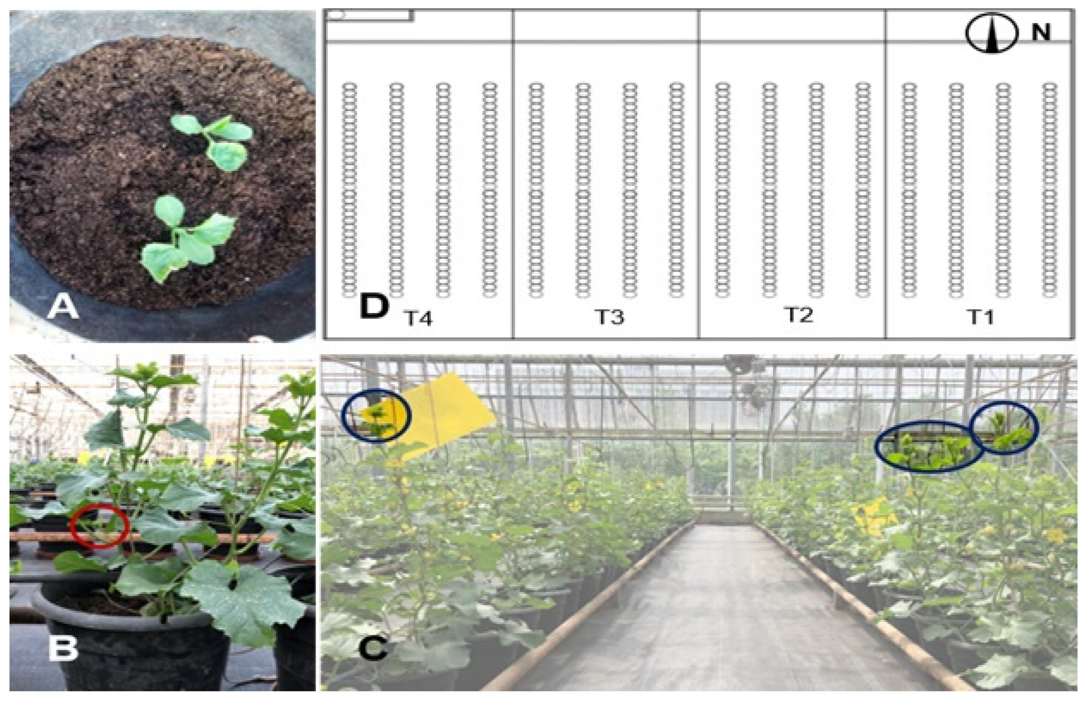
3.2. Leaf Image Acquisition

Images of upper leaf surfaces were taken by a single-lens reflex (SLR) camera (Canon EOS 5D Mark II, Japan) in a closed box of 60 cm × 60 cm × 60 cm. The camera settings were adjusted at M mode, exposure compensation set to zero, 1/320 shutter speed, 60 mm focal length and ISO 200. In the photo box, the light was evenly illuminated, and there was a fixed panel of light-emitting diode (LED) on the top two-sides of the photo box. Controlled LED power light was used with 60 W maximum value. Astral lamp panels (38 cm × 38 cm) were fixed to hold the leaves. The box opened at the top.
Finally, 624 digital images were taken from 156 plants’ samples. One image was taken from each of the four canopy leaves of the plant.

3.3. Collecting Meteorological Data of Greenhouse

After transplanting seedlings to the pots, environmental factors of the greenhouse, such as temperature and photosynthetically active radiation, were monitored by two portable automatic weather stations (HOBO-U30, Onset, Bourne, Ma, USA) in every 5 min.

3.4. Establishment of Machine Learning (ML) Model

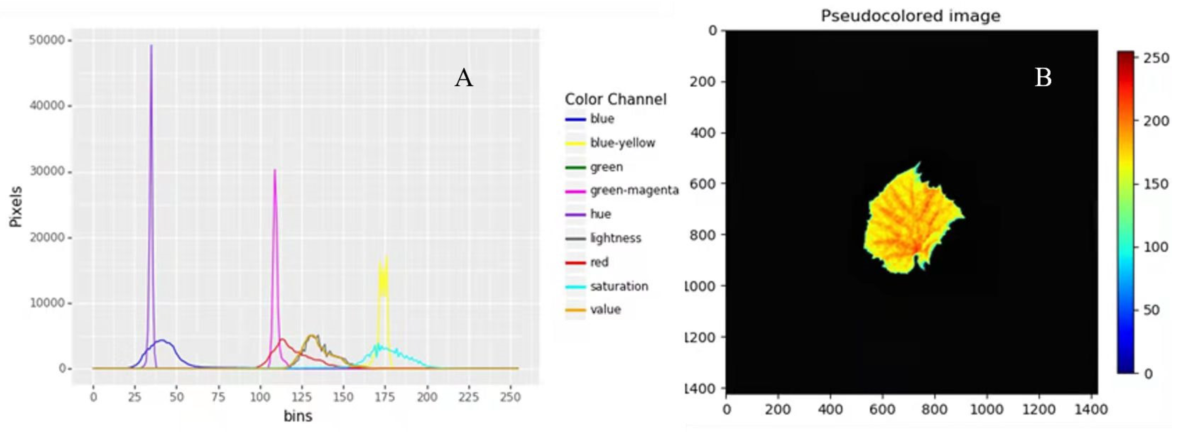
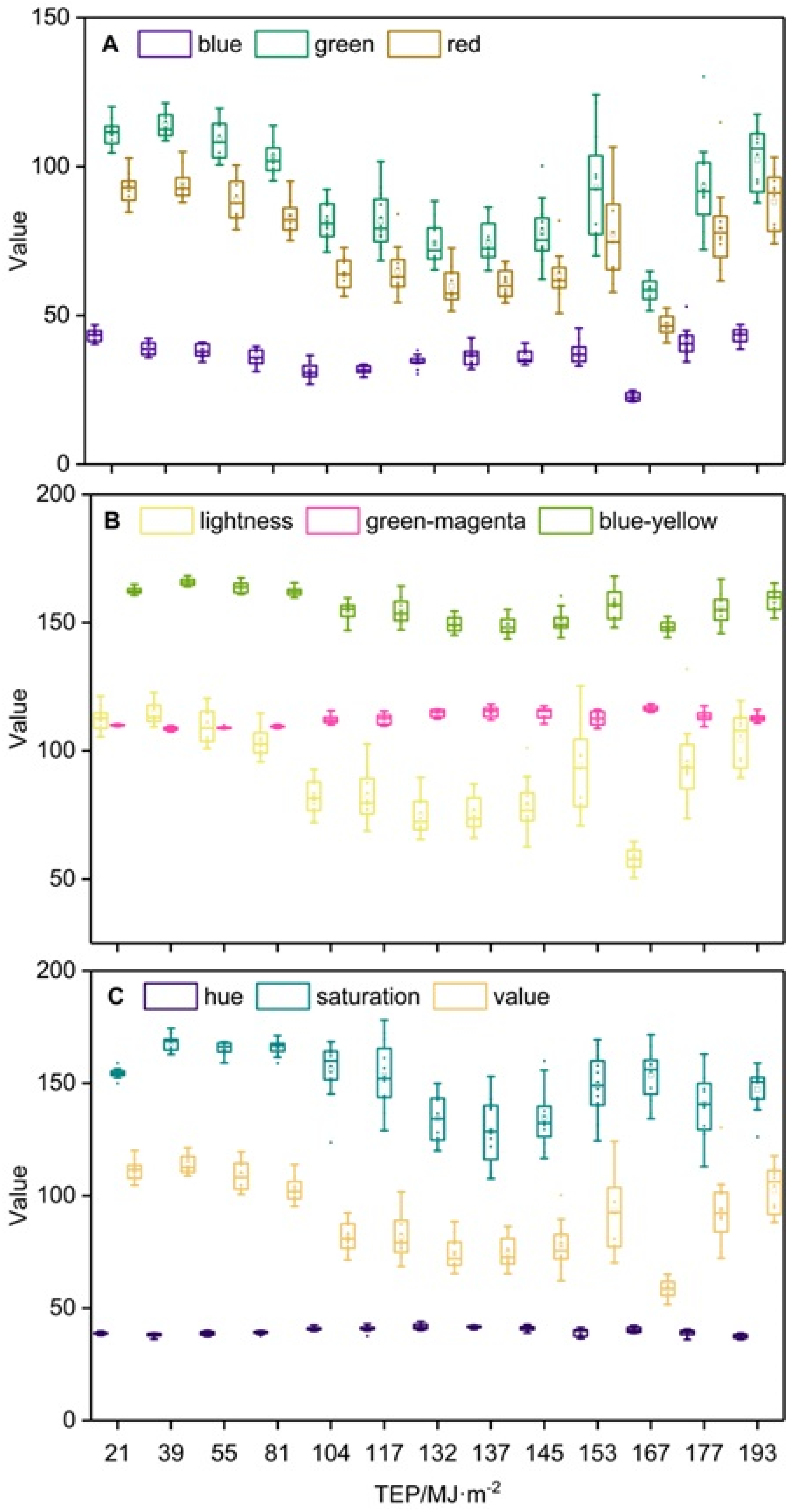
Extraction of Phenotypical Features

Phenotypic extraction parameters were used as conversion from visual characteristics of images into mathematical forms that could be recognized, processed and analyzed by a computer. In this study, the image-analysis software (PlantCV 3.2.0) was used for high-throughput plant phenotyping. PlantCV 3.2.0 is a modular open-source framework, which is written in Python [51].
Two steps were included in the visual digital images processing pipeline of PlantCV, which were used as segmented object (detection or isolation) and analysis (analysis of segmented objects). Taking a muskmelon plant as an example, we show the procedures of image processing in Figure 4. The procedures were as follows: (1) recognized the digital images; (2) converted color space from red green blue (RGB) to hue saturation value (HSV) and extracted saturation channel to get saturation threshold level; (3) removed the image noise with median filtering algorithm; (4) converted color space RGB to LAB and extracted blue channel to get blue threshold level image; (5) segmented the original image into the targeted region and object of interest based on the thresholds of saturation and blue-yellow images; (6) analyzed morphological features; (7) extracted color indexes based on color histogram and pseudo-colored image; (8) extracted the netting indexes based on gray-level co-occurrence matrix; and (9) extracted phenotypic parameters as output. Furthermore, a color histogram and pseudo-colored image of the fully expanded leaf are presented in Figure 5.
Thirty-one phenotypical parameters were extracted from each image and numbered 1 to 31 (Table 1), including 9 color parameters involved in 3 color spaces (RGB, LAB, and HSV), 16 morphological parameters based on contour tracking method, 6 netting characteristics parameters based on grey level co-occurrence matrix. All parameters contained means of four canopy leaves of plants.

4. Result

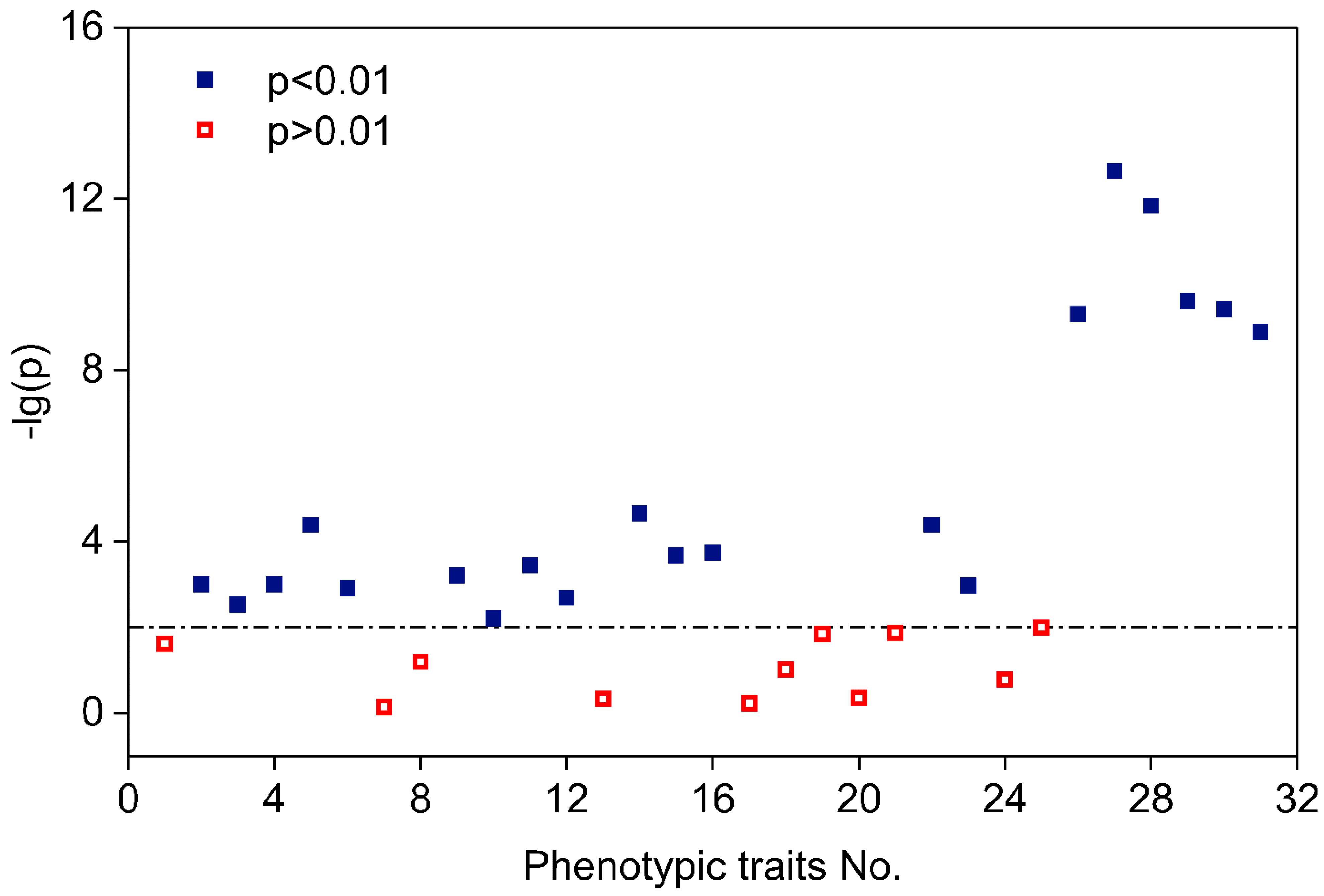
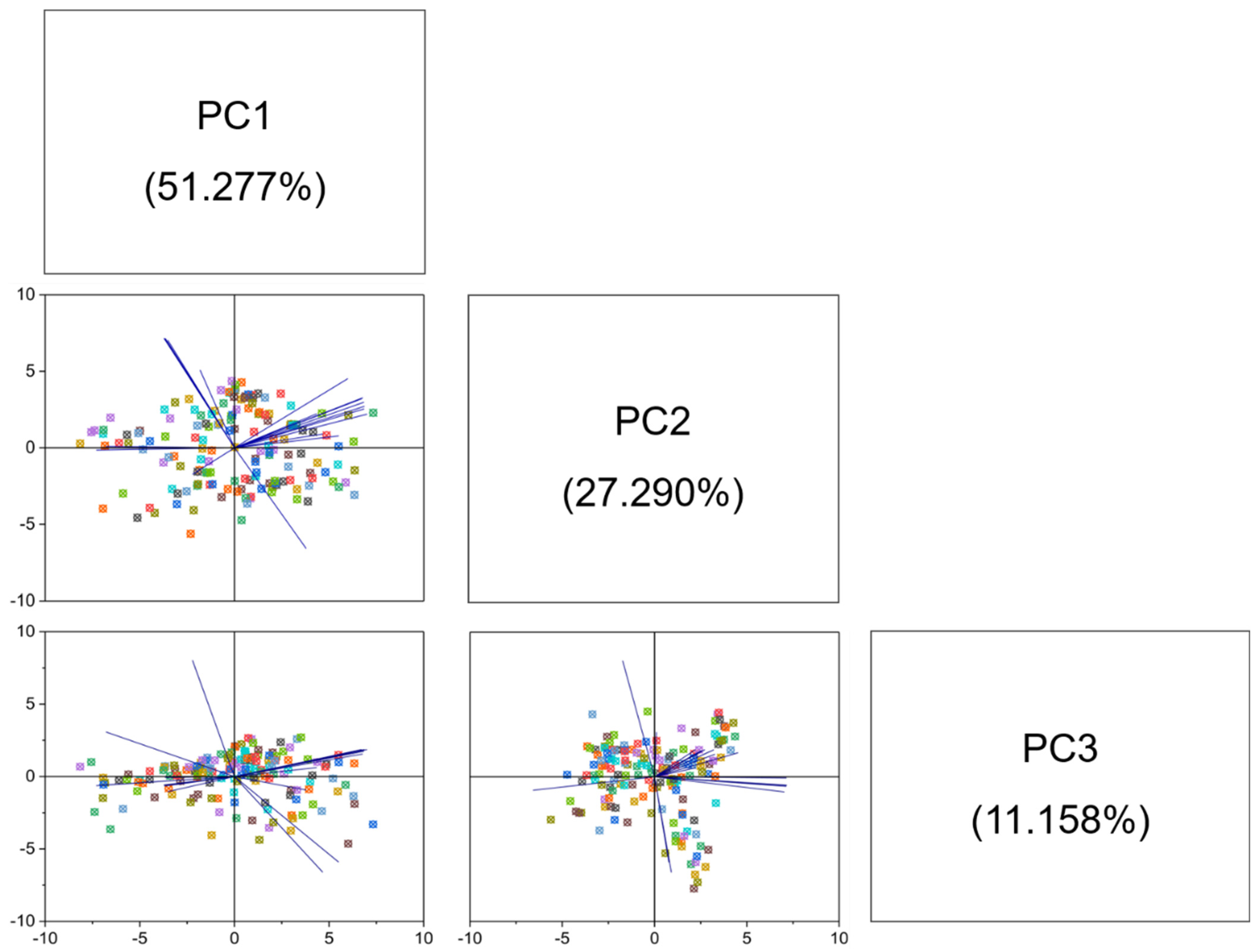
4.1. Phenotypical Feature Parameters Screening

One-way ANOVA: One-way ANOVA was performed to analyze the relationship between the extracted feature parameters and plant nitrogen concentration (Figure 6). Results highlighted three color indexes (1 blue, 7 hues and 8 saturation) and eight morphological feature indexes (13 perimeters, 17 center-of-masses-x, 18 center-of-masses-y, 19 hull-vertices, 20 ellipse-center-x, 21 ellipse-center-y, 24 ellipse-angle and 25 ellipse-eccentricity) were not associated with plant nitrogen concentration (p > 0.01). In contrast, the other 20 feature parameters were significantly correlated with the nitrogen concentration (p < 0.01). Thus, the 20 feature parameters were chosen for the construction of nitrogen nutrition diagnosis models.
Principal component analysis (PCA): PCA was further performed to reduce the above 20 screened feature parameters’ dimensions (Table 2). First, these 20 feature parameters were used to determine the sampling adequacy of data for analysis by Kaiser–Meyer–Olkin (KMO) test [53] and Bartlett spherical test [54], using SPSS Statistics version 22.0. The results indicate that the images’ data obtained adequate results (KMO = 0.797), and both the correlations and partial correlations between these parameters were significant (p = 0). Then, PCA was performed to select the principal components whose eigenvalues were more than 1, and only three principal components showed eigenvalues more than 1 (Figure 7). The scatter plots showed projections of the top three PCs based on the PCA of images-based dataset. The component scores (shown in points) were presented as different colors with the same shape, according to the phenotypical features. The component loading vectors (represented in lines) of all features were superimposed proportionally to their contributions. The contribution rates of PC1, PC2 and PC3 are 51.277%, 27.290% and 11.158%, respectively; namely, a total contribution rate of 89.725% was reached. The three principal components could be used as an input variable for nutrient diagnosis models, indicating the input data dimension as a reduction from 20 to 3.

4.2. Establishment of Backpropagation Neural Network (BPNN)

Backpropagation neural network (BPNN) was trained as a two-layer forward neural network by using a backpropagation algorithm [55]. It is one of the most widely used and most mature machine learning model. The architecture consisted of three parts: input layer, hidden layer and output layer. Three principal components were used as input that were considered as the input layer, and the nitrogen concentration of corresponding plants was obtained as input which was considered as output in the model. Thus, the input node was set to 3, the output node was set to 1 and the hidden neuron node was calculated according to Empirical Formula (1):
l < a + m + n
where n, l and m represent input layer, hidden layer and output layer, respectively; a is a constant with range within 0–10.
A random 80% of the total dataset (124 plants) was used as the training dataset, and the other 20% (32 plants) was used as the test dataset. In a MATLAB R2016a based on BPNN, used after a series of tests to debug the parameters of BPNN, we normalized input data by mapminmax () function, selected logsid () function as the activation function and adopted the variable learning rate to the learning algorithm in the model. The maximum learning rate was 0.2, the minimum learning rate was 0.02 and the momentum learning rate was 0.02 (Codes in Supplementary Materials S1).

4.3. Establishment of Deep Learning Models

In deep learning, the models were established by using Python 3.6.5 programming language and Keras 2.1.2. Keras 2.1.2 [56] is a high-level neural network API that is written in Python and capable of running on the top of TensorFlow 1.6.0 [57].

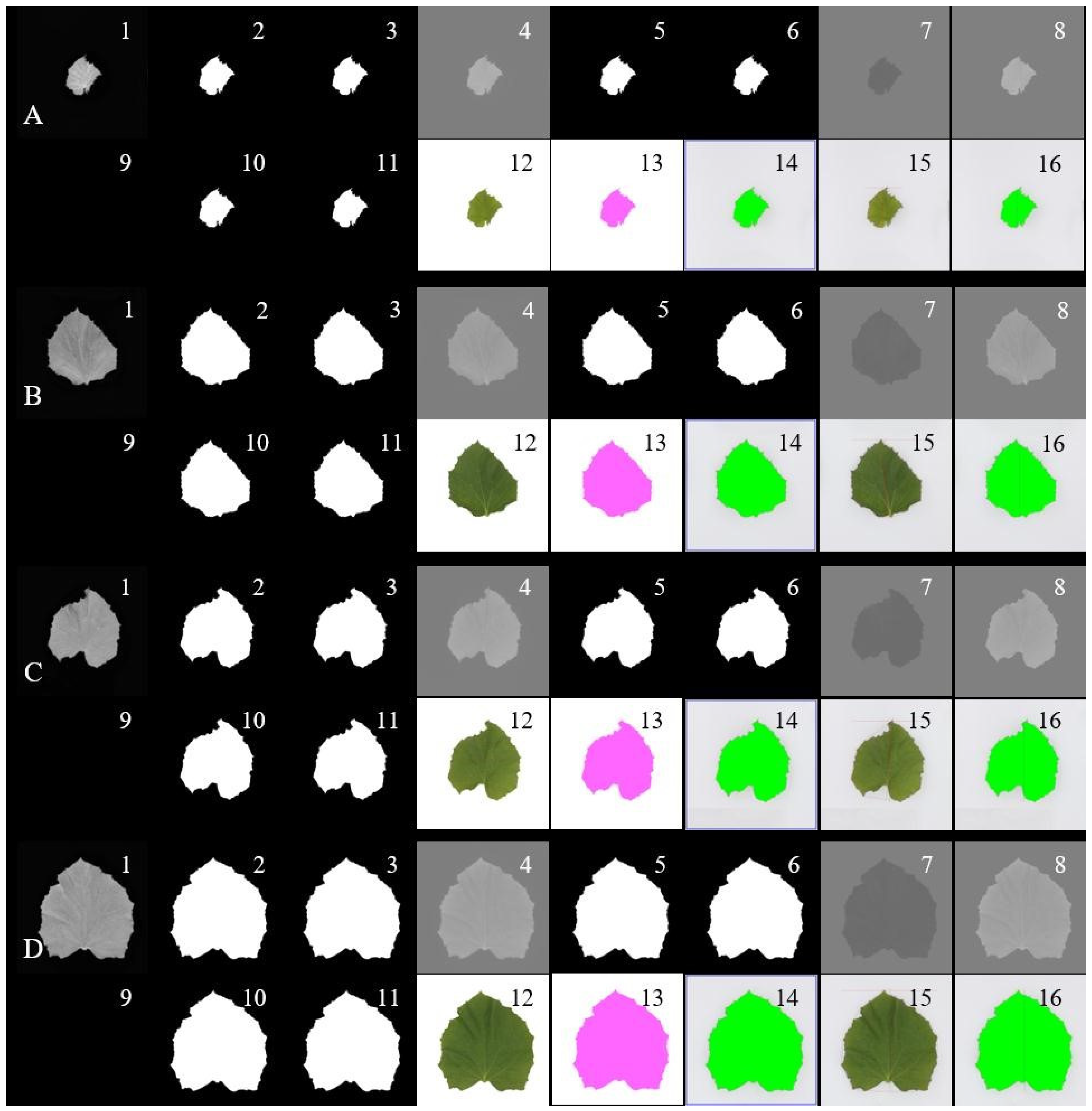
4.3.1. Image Preprocessing

First, each leaf image was annotated to correspond the leaf nitrogen concentration. Then the 624 original leaf images were amplified through rotating the original images at 5 random angles, and finally 3744 images in total were obtained for analysis. After splicing the images of four leaves of a plant together, then 936 new images were used as an input dataset of the neural network, while the image resolution changed from 128 × 128 to 256 × 256. The measured nitrogen concentration was still put as the output dataset. The input and output datasets were randomly divided into a training subset (80%), cross-validation subset (10%) and test subset (10%).

4.3.2. Data Preprocessing of Environmental Factors

The growth rate of plants was mainly determined by the relative thermal effectiveness (RTE) of temperature and photosynthetic active radiation (PAR). The growth and development of netted melon in greenhouse is a dynamic process that changes with time. If the planting days are used to predict the growth and development of the crop at a certain time node, and the influence of the temperature and light as environmental factor due to specific plant location cannot ignore for plant growth and development. In addition, meteorological and environmental data also affect the phenotype (such as color) of plant leaves. As the accumulated total production of thermal effectiveness and PAR gradually increased in the cultivation condition in this study. For the RGB color space, the blue value changed smoothly, and the red and green values both increased first, then decreased and then again increased, represented as green > red > blue (Figure 8A); meanwhile, for the LAB color space, the green-magenta value hardly changed, but the blue-yellow and lightness values both showed a slight increase, then decreased and then again increased, but the blue-yellow value changed a little, and the lightness value fluctuated widely, represented as blue-yellow > green-magenta > lightness (Figure 8B). For the HSV color space, the hue value showed almost no change; the saturation and value values both showed a trend of first increasing, then decreasing and then again increasing, represented as saturation > value > hue (Figure 8C).
Therefore, this study used the light–temperature index radiant thermal product TEP instead of planting days as a time series variable and combined them with images data to predict the growth and development stage of greenhouse netted muskmelon and plants’ nitrogen concentrations. We measured the cumulative radiant heat product of the plant at each sampling time [58] and annotated it into the corresponding canopy leaf images as the environmental input variable of the neural network.

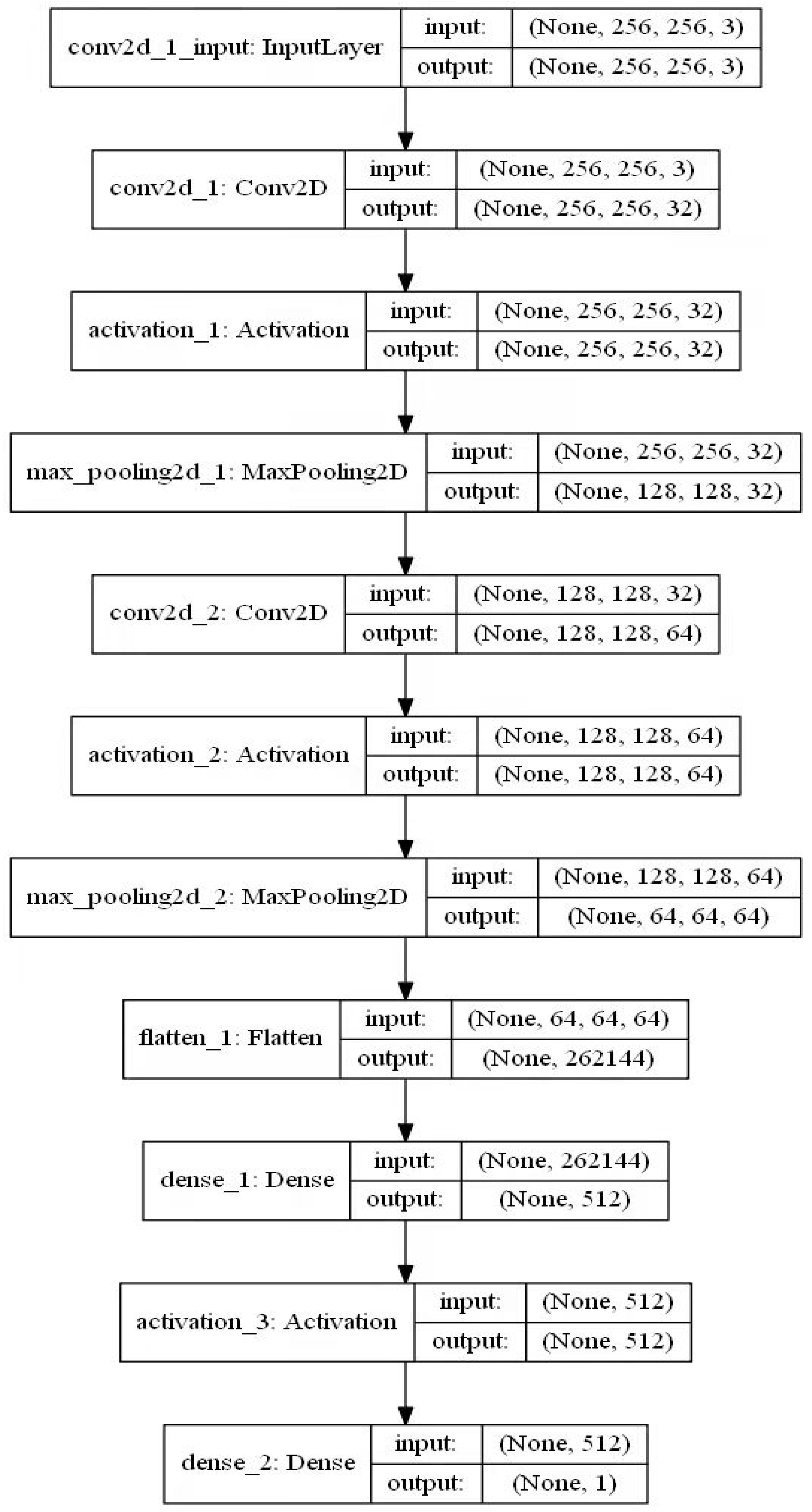
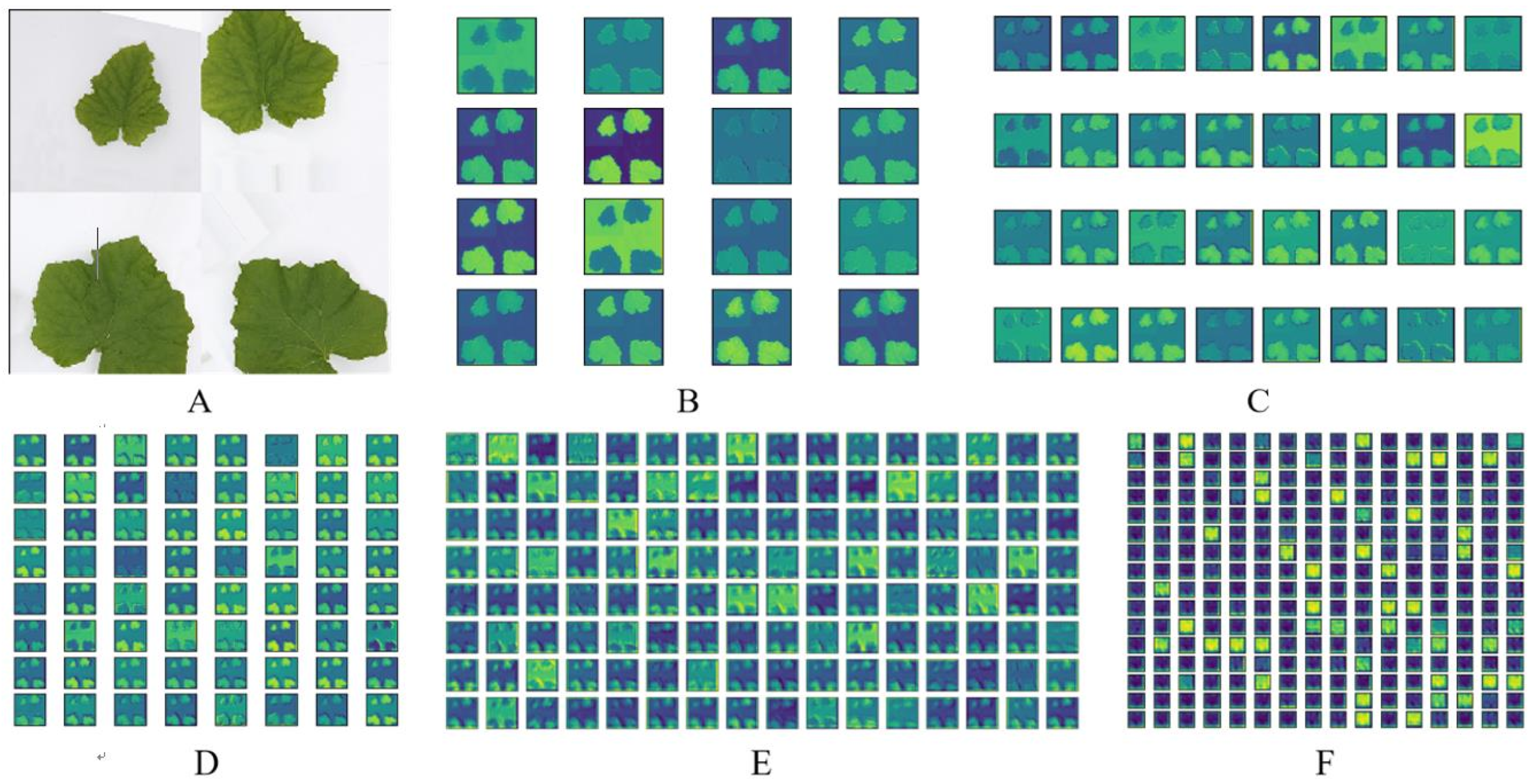
4.4. Establishment of CNN Model

In deep learning, a convolution neural network (CNN) is a class of feed forward neural networks and most commonly applied to analyze visual images. CNN employs convolution operation in place of general matrix multiplication operation at least one of their layers. CNN generally consists of an input layer, output layer, and multiple hidden layers, such as convolutional layers, pooling layers, and fully connected layers. The pooling layers are connected with all the neurons of the convolutional layers [59].
We set two convolutional layers, two pooling layers and two fully connected layers in the CNN model by using LeNet as the backbone. In the convolution layers, kernel size was 5 and padding was set as “same”. In pooling layers, pool size and strides were both (2, 2), rectified linear units (ReLU) were set as the activation function, Adam () was set as the optimizer and batch size was kept as 12 (Codes in Supplementary Materials S2). The input volumes and output volumes of every layer are presented in Figure 9. The R2 and MSE methods were used for model evaluation.

4.5. Establishment of DCNN Model

Based on CNN architecture, three convolutional layers, three pooling layers and three fully connected layers were supplied to build up a deep-learning convolution neural network (DCNN) model. Different filters in the convolutional layer had placed for other parameters. After a series of convolution, pooling and activation operations in the network, the features of input images were detected and learned. The feature maps of essential areas of the image out of each of the middle layers are presented in Figure 10. With the increased of network depth, the extracted features became more filtered and gave more precise extracted feature parameters. The high activation layer carried more targeted information: the valuable information was enlarged and refined, while the irrelevant information was filtered out (Codes in Supplementary Materials S3). However, in CNN, the too-deep neural network presented results with less prediction accuracy, excessive calculation time and over-fitting, while, in DCNN, the results presented more predication accuracy in less calculation time, without over-fitting. The parameters were set in DCNN as the same in the CNN model.

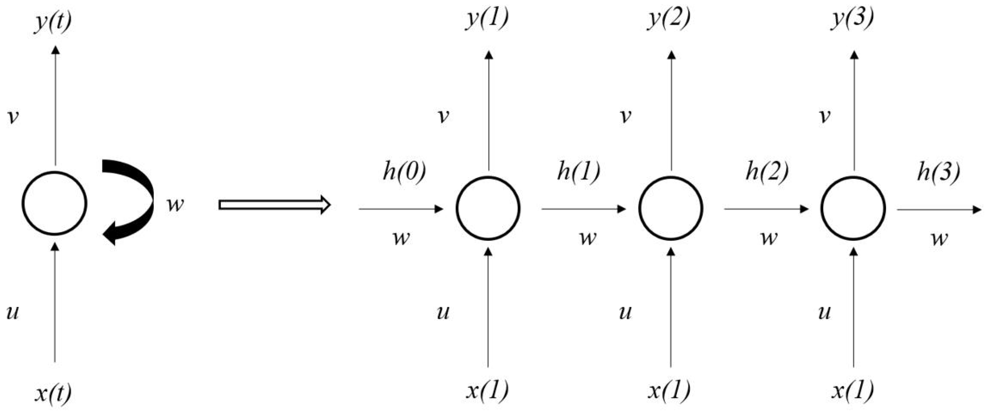
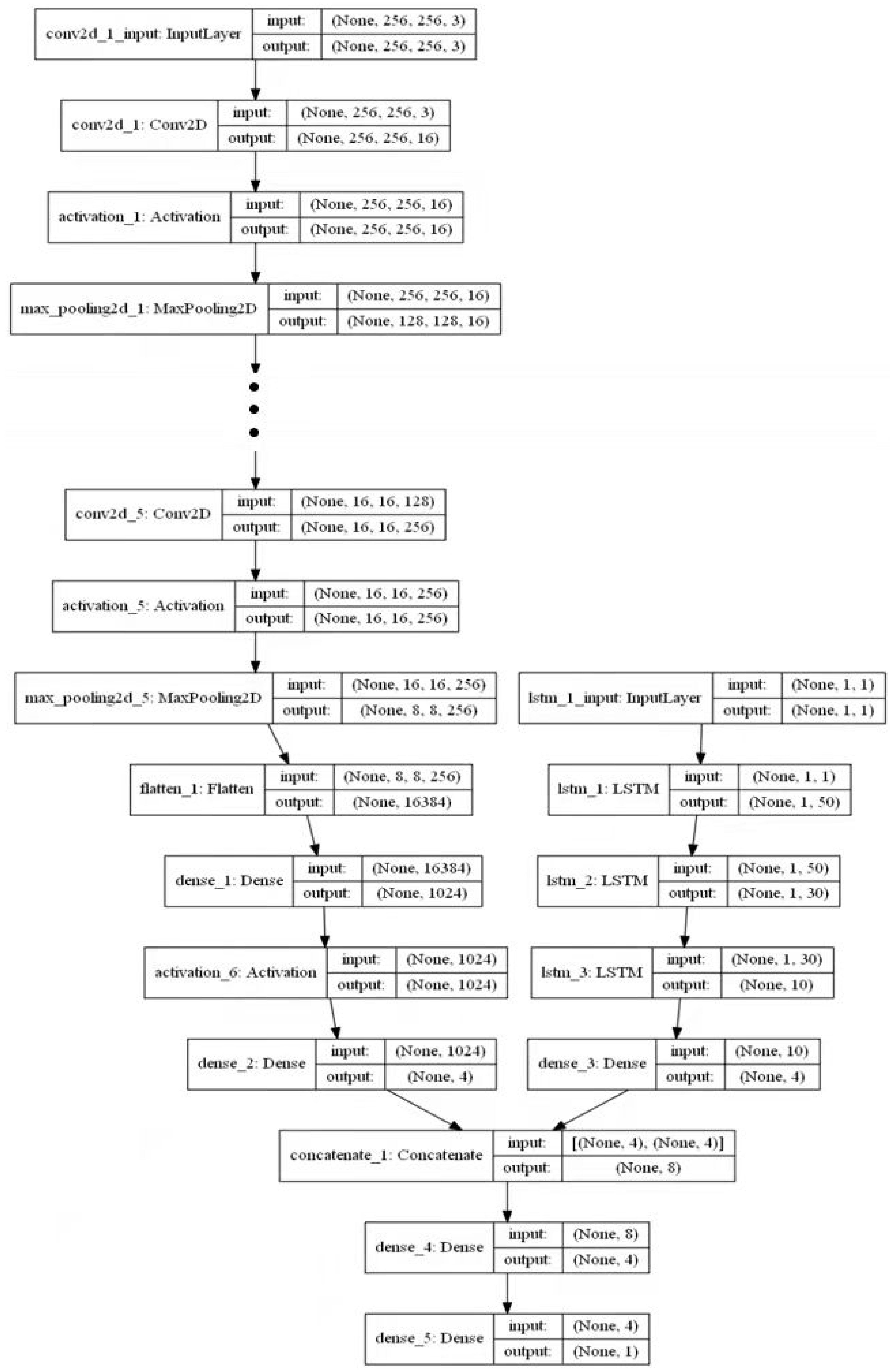
4.6. Establishment of DCNN–LSTM Model

A recurrent neural network (RNN) is a class of neural networks that utilizes input data in series. The architectures (Figure 11) are considered as flexible and used in speech recognition, machine translation, emotion analysis and picture description. The input volume can be used as a series of text, speech, time, etc., that depends on previous elements. The time steps at the same state (input, output and hidden conditions) share one weight matrix, which greatly reduces the number of parameters to be learned in the model.
Long short-term memory (LSTM) is a variant of RNN that can learn long-term dependence. It is the most widely used type of RNN. Compared with the traditional RNN, LSTM introduces controllable self-cycling, which is more suitable for processing and predicting important events with relatively long intervals or delays in time series. The network solves problems, such as gradient disappearance and gradient explosion caused by time backpropagation during training [60]. The LSTM schematic view is shown in Figure 12.
A hybrid neural network model based on DCNN and LSTM was built (Codes in Supplementary Materials S4), and shown in Figure 13. The structure of DCNN showed consistency with increasing the number of hidden layers in the establishment of the CNN model. The LSTM part had put three layers and function as stateful = False. To make hybrid neural network, two fully connected layers of DCNN and LSTM models are put as an output with ReLU and linear functions as the activation function in the model. The leaf-image dataset was put as input from the DCNN part, the TEP dataset was put as input from the LSTM part in the hybrid neural network model and then the nitrogen concentrations of muskmelon plants were predicted. The R2 and MSE method were used for the model evaluation.

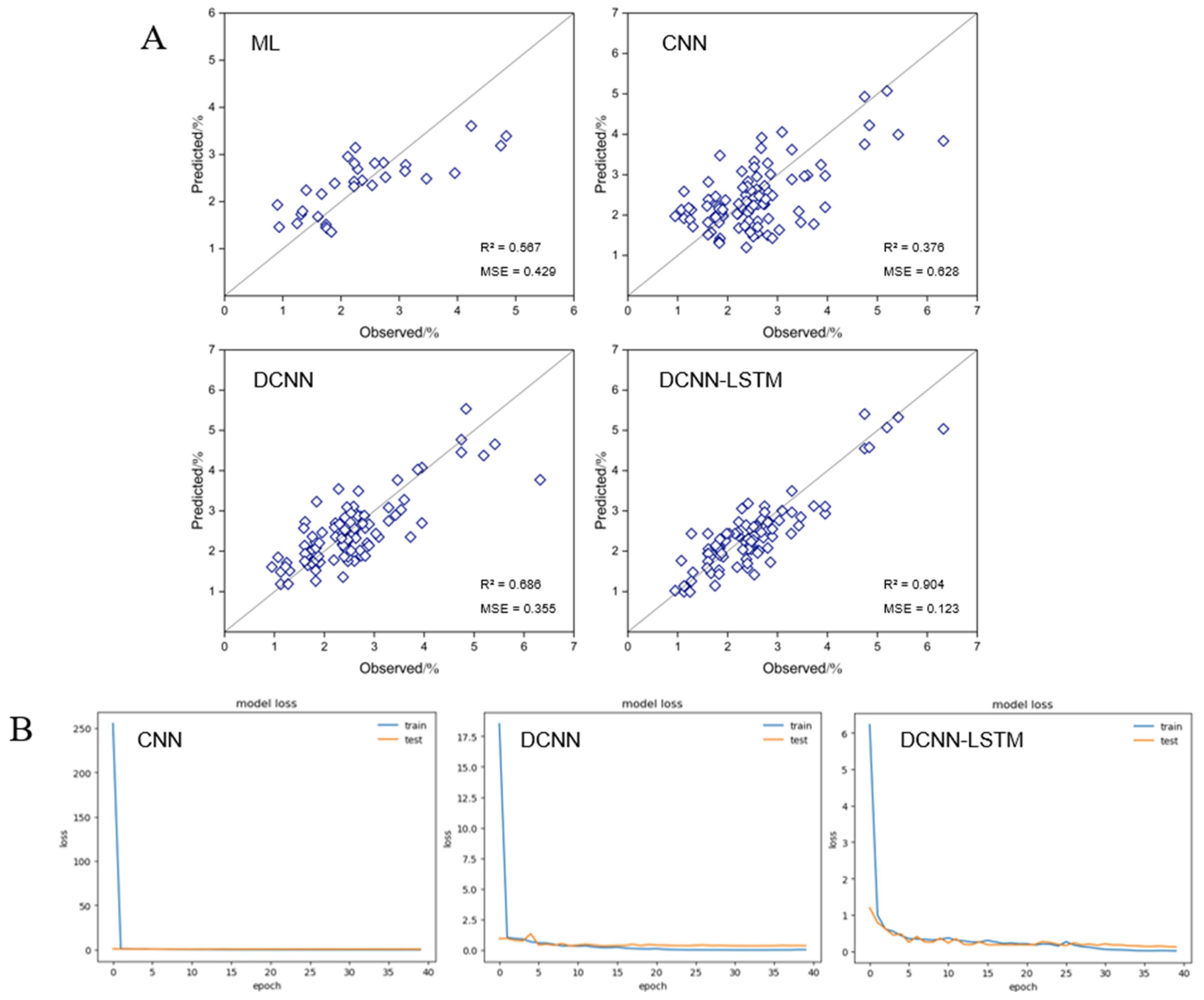
4.7. Evaluation of Models

The adjusted determination coefficient (R2) and mean square error (MSE) between predicted and measured values were used for model evaluation. In general, the higher R2 value and the lower MSE are considered as more accurate and the best model.
The calculation formulas were put as follows:
R 2 = i = 1 n ( y ^ i y ¯ ) 2 i = 1 n ( y i y ¯ ) 2
MSE = 1 n i = 1 n ( y i y i ^ ) 2
where y i   represents the measured value, y ^ i   represents the predicted value, y ¯ is the mean of measured values and n represents the sample number.
ML, DCNN and DCNN–LSTM were optimized to diagnose nitrogen concentration in muskmelon plants. A 1:1 scatter diagram of the predicted values and the measured values were plotted to evaluate models’ precision (Figure 14A). Evaluation results were shown as R2 = 0.567 and MSE = 0.429 for the BPNN model, R2 = 0.376 and MSE = 0.628 for R2 = 0.686 for the CNN model, R2 = 0.686 and MSE = 0.355 for the DCNN model, and R2 = 0.904 and MSE = 0.123 for the DCNN–LSTM model. With mean square error (MSE) as the loss function, the loss results of three deep learning models (DCNN and DCNN–LSTM) are shown in Figure 14B. For all models, the prediction accuracy improved to some extent with the increase of iterative training, but after reaching a certain number of trainings, the accuracy did not show a significant increase, or even decrease. At the same time, the more iterative training times required more time for model calculation. For the deep learning model, the model loss was very high in the initial iterative training. With the increase of the number of training iterations, the training sets in model loss showed a sharp drop in the beginning, but later did not show decline in falling and tended to the flat. The model loss of the test set also gradually decreased, but later tended to the flat and showed similar trends of the training set of model loss. In general, the test set was shown to have slightly higher model loss than the training set.

5. Discussion

In the present study, we collected the digital images of canopy leaves and meteorological data during the whole growth period of muskmelon in the greenhouse. Using these data, plant nitrogen nutrition diagnosis models were built based on machine learning or deep learning. The first model (BPNN (R2 = 0.567, MSE = 0.429) was constructed by adopting machine vision technology to extract and process the phenotypic features of leaf images. Then a CNN nitrogen nutrition diagnosis model (R2 = 0.376, MSE = 0.628) was constructed. For the CNN model, the original leaf image was directly put as input into the model and preprocessed. By increasing the depth of CNN, we built DCNN (R2 = 0.686, MSE = 0.355) for nitrogen nutrition diagnosis. Furthermore, based on DCNN, a hybrid model, namely DCNN–LSTM, was constructed, and R2 = 0.904 and MSE = 0.123 were used as the evaluation indexes’ values. For the model, TEP, instead of time series, was used as a time variable.
Many emerging technologies have been applied to crop nitrogen nutrition diagnosis [8]. Based on the spectral information or digital images, the nitrogen nutrition status of rice [61,62], wheat [17,63] and corn [64] has been predicted. These studies only statistically analyze the relationship between reflectance spectrums, phenotypes, plant growth and physiological characteristics [15,65] through simplifying the deduction process and improving the calculation efficiency and accuracy by using a numerical optimization algorithm, PCA, neural networks, etc. Such an idea is adopted in this study for models’ construction. The distribution of nitrogen at different canopy heights did not show uniformity [66], and the correlation between nitrogen concentration, spectral and fluorescence characteristics of extra vertical heights also showed difference [67]. Hu et al. [49] reported that the SPAD values of three apical leaves of melon showed the highest correlation with the nitrogen content in leaves, which showed suitability for the diagnosis of nitrogen nutrition, and indicating that it was feasible to predict the nitrogen content of the whole plant through the canopy leaves. Padilla et al. [35] predicted the nitrogen nutrition index (NNI) of muskmelon by using the canopy reflectance characteristics of plants by optical sensor, the flavonol and chlorophyll contents in the leaves also determined to evaluate the nitrogen status. NNI refers to the ratio of the actual nitrogen concentration in the upper part of the crop to the critical nitrogen concentration under the corresponding biomass. It is one of the basic method to judge the crops’ nitrogen profit and loss level [52,68]. To measure the actual nitrogen concentration in the crops are considered as the premise of calculating NNI, but the above research could directly predict the nitrogen concentration in plants.
Compared with traditional machine-learning-based models, deep-learning-based models’ virtue is considered as an approaches to avoid the manual handcrafting and the problems of inconsistent criteria in parameters [69]. Machine-learning-based models are considered as a reliable technology for selecting parameters, reducing dimensions and then decreasing the number of neural network nodes. Nevertheless, the input-data information is reduced and further lowers the accuracy of the predicted values. Deep-learning-based models overcome the disadvantage through inputting the original images’ information directly in the model. In such a way, adequate original information improved the accuracy of output in the model.
The deep learning approaches are booming in the plant community, and this proves that it has a great potential in agriculture. It has been widely used in species identification [70], pests detection [71] and yield prediction [72] of horticultural crops. CNN is the most commonly used deep-learning-based technology, in which the plant features extracted by using deep neural network are better than the artificial design. This is confirmed and verified briefly by the better performance of the deep learning model. In terms of prediction accuracy, the hybrid model DCNN–LSTM was the best among the four models, followed by DCNN, BPNN and CNN, in our study. DCNN is a machine learning-based model, but it shows higher prediction accuracy than the deep-learning-based model BPNN. This indicates that the machine-learning-based model is not necessarily considered less than deep-learning-based models based on prediction accuracy. If machine learning approaches are combined with proper parameters, trained with adequate data and have less of a loss of information, then high prediction accuracy can be obtained. While deep learning techniques are less costly and have more efficiency to get an output results in less time as compared to machine learning parameters.
Similarly, DCNN–LSTM was the best deep learning-based model followed by DCNN and the CNN was at the bottom. DCNN–LSTM is presented the most reliable and applicable model among the three models and has shown the highest prediction accuracy, combining with real-time leaf images and environmental factors. The model can be improved and used in other fields of agriculture. Previously, Schmidhuber [19] combined CNN and LSTM to predict soybean yield, with a histogram of the whole images as an input dataset. Ghazaryan et al. [73] estimated crop yield by using multi-source satellite image series and deep learning, the CNN–LSTM model presented the highest accuracy results. Namin et al. [30] improved the plant classification by using time series with digital images of various genotypes of Arabidopsis in the CNN–LSTM model on the basis of accuracy. Haryono et al. [74] used CNN–LSTM methods for identification and authentication of the herbal leaves with an accuracy of 94.96%. Baek et al. [75] presented by combine use of CNN and LSTM networks for simulating water quality including total nitrogen, total phosphorous, and total organic carbon. It was concluded that the proposed approach CNN–LSTM could be used accurately in simulating the water level and water quality. Sun et al. [76] used the deep CNN–LSTM model to predict soybean yield on the county level. The results indicated that the prediction performance of the proposed deep CNN–LSTM model showed outstanding performance from the pure CNN or LSTM model in both end-of-season and in-season. Recent experiments in this area suggested that CNN could explore more phenotype features and LSTM showed the ability to reveal phenotypic characteristics. So, deep CNN and LSTM both play an important role in crop nitrogen prediction. The accumulation of environmental data could be used to study the relationship between phenotype changes and nitrogen concentration during crop growth process. In our study, TEP values used as time series, the prediction accuracy of LSTM model is also improved and indicating that TEP values are a good substitute for time series. Thus, our constructed nitrogen nutrition diagnosis models presented timely and accurately providing an excellent way of prediction for nitrogen nutrition management in muskmelon production.
However, this study had some limitations: the image data were not adequate in the experiment. In the future, we can use the method of increasing sample size, melon varieties and cultivation environments to establish a more applicable, reliable and stable model.

6. Conclusions

In conclusion, this study provides the knowledge for the diagnosis of nitrogen nutrition for greenhouse muskmelon by using machine-learning-based and deep-learning-based models. A hybrid model, DCNN–LSTM, which combines real-time digital images with meteorological factors, shows the highest accuracy (R2 = 0.686, MSE = 0.355) in the prediction of plant nitrogen concentration in muskmelon production in the greenhouse. These findings indicate the great potential of deep learning technology in crop nutrition diagnosis and provide a technique and reference for real-time, convenient, accurate and nondestructive nitrogen nutrition diagnosis in greenhouse muskmelon production. The study lays the foundation for the intelligent monitoring of nitrogen nutrition in plants.

Supplementary Materials

The following are available online at https://www.mdpi.com/article/10.3390/horticulturae7110489/s1, Supplementary data S1 ǀ BPNN model code for muskmelon, Supplementary data S2 ǀ CNN model code for muskmelon, Supplementary data S3 ǀ DCNN model code for muskmelon, Supplementary data S4 ǀ DCNN-LSTM model code for muskmelon.

Author Contributions

L.C. and Q.N. designed research; D.L. and Y.Y. performed research; D.L. and Y.Y. analyzed data; D.L., Y.Y., M.K.H. and D.H. wrote and revised the paper. All authors have read and agreed to the published version of the manuscript.

Funding

This work was financially supported by the National Natural Science Foundation of China (NSFC) (Project No. 31471411), the Technology System of Melons and Fruits Production of Shanghai, Study on the High-efficient Selection and Cultivation Techniques for Specialty Vegetable (Grant Nos. T201701-4).

Institutional Review Board Statement

Not applicable.

Informed Consent Statement

Not applicable.

Data Availability Statement

We have provided data in supplementary materials.

Acknowledgments

The authors would like to acknowledge the National Natural Science Foundation of China for their support.

Conflicts of Interest

The authors declare no conflict of interest.

References

  1. Gallardo, M.; Gimenez, C.; Martinez-Gaitan, C.; Stoeckle, C.O.; Thompson, R.B.; Granados, M.R. Evaluation of the VegSyst model with muskmelon to simulate crop growth, nitrogen uptake and evapotranspiration. Agric. Water Manag. 2011, 101, 107–117. [Google Scholar] [CrossRef]
  2. Kirnak, H.; Higgs, D.; Kaya, C.; Tas, I. Effects of irrigation and nitrogen rates on growth, yield, and quality of muskmelon in semiarid regions. J. Plant Nutr. 2005, 28, 621–638. [Google Scholar] [CrossRef]
  3. Li, D.; Li, C.; Yao, Y.; Li, M.; Liu, L. Modern imaging techniques in plant nutrition analysis: A review. Comput. Electron. Agric. 2020, 174, 105459. [Google Scholar] [CrossRef]
  4. Fredes, A.; Sales, C.; Barreda, M.; Valcarcel, M.; Rosello, S.; Beltran, J. Quantification of prominent volatile compounds responsible for muskmelon and watermelon aroma by purge and trap extraction followed by gas chromatography-mass spectrometry determination. Food Chem. 2016, 190, 689–700. [Google Scholar] [CrossRef] [PubMed] [Green Version]
  5. Song, S.; Lehne, P.; Le, J.; Ge, T.; Huang, D. Yield, fruit quality and nitrogen uptake of organically and conventionally grown muskmelon with different inputs of nitrogen, phosphorus, and potassium. J. Plant Nutr. 2010, 33, 130–141. [Google Scholar] [CrossRef]
  6. Li, X.; Hu, C.; Delgado, J.A.; Zhang, Y.; Ouyang, Z. Increased nitrogen use efficiencies as a key mitigation alternative to reduce nitrate leaching in north China plain. Agric. Water Manag. 2007, 89, 137–147. [Google Scholar] [CrossRef]
  7. Galloway, J.N.; Dentener, F.J.; Capone, D.G.; Boyer, E.W.; Howarth, R.W.; Seitzinger, S.P.; Asner, G.P.; Cleveland, C.C.; Green, P.A.; Holland, E.A.; et al. Nitrogen cycles: Past, present, and future. Biogeochemistry 2004, 70, 153–226. [Google Scholar] [CrossRef]
  8. Shi, Y.; Zhu, Y.; Wang, X.; Sun, X.; Ding, Y.; Cao, W.; Hu, Z. Progress and development on biological information of crop phenotype research applied to real-time variable-rate fertilization. Plant Methods 2020, 16, 11. [Google Scholar] [CrossRef]
  9. Li, D.; Wang, X.; Zheng, H.; Zhou, K.; Yao, X.; Tian, Y.; Zhu, Y.; Cao, W.; Cheng, T. Estimation of area and mass-based leaf nitrogen contents of wheat and rice crops from water-removed spectra using continuous wavelet analysis. Plant Methods 2018, 14, 76. [Google Scholar] [CrossRef]
  10. Padilla, F.M.; Peña-Fleitas, M.T.; Gallardo, M.; Thompson, R.B. Proximal optical sensing of cucumber crop N status using chlorophyll fluorescence indices. Eur. J. Agron. 2016, 73, 83–97. [Google Scholar] [CrossRef]
  11. Pandey, P.; Ge, Y.; Stoerger, V.; Schnable, J.C. High Throughput In vivo Analysis of Plant Leaf Chemical Properties Using Hyperspectral Imaging. Front. Plant Sci. 2017, 8, 1348. [Google Scholar] [CrossRef] [Green Version]
  12. Agati, G.; Foschi, L.; Grossi, N.; Volterrani, M. In field non-invasive sensing of the nitrogen status in hybrid bermudagrass (Cynodon dactylon × C. transvaalensis Burtt Davy) by a fluorescence-based method. Eur. J. Agron. 2015, 63, 89–96. [Google Scholar] [CrossRef]
  13. Chen, D.; Shi, R.; Pape, J.M.; Neumann, K.; Arend, D.; Graner, A.; Chen, M.; Klukas, C. Predicting plant biomass accumulation from image-derived parameters. Gigascience 2018, 7, 1–13. [Google Scholar] [CrossRef] [Green Version]
  14. Fernández-Pacheco, D.G.; Escarabajal-Henarejos, D.; Ruiz-Canales, A.; Conesa, J.; Molina-Martínez, J.M. A digital image-processing-based method for determining the crop coefficient of lettuce crops in the southeast of Spain. Biosyst. Eng. 2014, 117, 23–34. [Google Scholar] [CrossRef]
  15. Guo, D.; Juan, J.; Chang, L.; Zhang, J.; Huang, D. Discrimination of plant root zone water status in greenhouse production based on phenotyping and machine learning techniques. Sci. Rep. 2017, 7, 8303. [Google Scholar] [CrossRef] [Green Version]
  16. Neilson, E.H.; Edwards, A.M.; Blomstedt, C.K.; Berger, B.; Moller, B.L.; Gleadow, R.M. Utilization of a high-throughput shoot imaging system to examine the dynamic phenotypic responses of a C-4 cereal crop plant to nitrogen and water deficiency over time. J. Exp. Bot. 2015, 66, 1817–1832. [Google Scholar] [CrossRef]
  17. Baresel, J.P.; Rischbeck, P.; Hu, Y.; Kipp, S.; Hu, Y.; Barmeier, G.; Mistele, B.; Schmidhalter, U. Use of a digital camera as alternative method for non-destructive detection of the leaf chlorophyll content and the nitrogen nutrition status in wheat. Comput. Electron. Agric. 2017, 140, 25–33. [Google Scholar] [CrossRef]
  18. Sethy, P.K.; Barpanda, N.K.; Rath, A.K.; Behera, S.K. Nitrogen deficiency prediction of rice crop based on convolutional neural network. J. Ambient Intell. Humaniz. Comput. 2020, 11, 5703–5711. [Google Scholar] [CrossRef]
  19. Schmidhuber, J. Deep learning in neural networks: An overview. Neural Netw. 2015, 61, 85–117. [Google Scholar] [CrossRef] [Green Version]
  20. Chen, J.D.; Chen, J.X.; Zhang, D.F.; Sun, Y.D.; Nanehkaran, Y.A. Using deep transfer learning for image-based plant disease identification. Comput. Electron. Agric. 2020, 173, 11. [Google Scholar] [CrossRef]
  21. Dyrmann, M.; Karstoft, H.; Midtiby, H.S. Plant species classification using deep convolutional neural network. Biosyst. Eng. 2016, 151, 72–80. [Google Scholar] [CrossRef]
  22. Grinblat, G.L.; Uzal, L.C.; Larese, M.G.; Granitto, P.M. Deep learning for plant identification using vein morphological patterns. Comput. Electron. Agric. 2016, 127, 418–424. [Google Scholar] [CrossRef] [Green Version]
  23. Kawasaki, Y.; Uga, H.; Kagiwada, S.; Iyatomi, H. Basic study of automated diagnosis of viral plant diseases using convolutional neural networks. In International Symposium on Visual Computing; Springer: Cham, Switzerland, 2015; pp. 638–645. [Google Scholar]
  24. Ma, J.; Du, K.; Zheng, F.; Zhang, L.; Gong, Z.; Sun, Z. A recognition method for cucumber diseases using leaf symptom images based on deep convolutional neural network. Comput. Electron. Agric. 2018, 154, 18–24. [Google Scholar] [CrossRef]
  25. Khaki, S.; Wang, L. Crop Yield Prediction Using Deep Neural Networks. Front. Plant Sci. 2019, 10, 621. [Google Scholar] [CrossRef] [Green Version]
  26. Madec, S.; Jin, X.; Lu, H.; De-Solan, B.; Liu, S.; Duyme, F.; Heritier, E.; Baret, F. Ear density estimation from high resolution RGB imagery using deep learning technique. Agric. For. Meteorol. 2019, 264, 225–234. [Google Scholar] [CrossRef]
  27. Rahnemoonfar, M.; Sheppard, C. Deep Count: Fruit Counting Based on Deep Simulated Learning. Sensors 2017, 17, 905. [Google Scholar] [CrossRef] [Green Version]
  28. Le, N.Q.K.; Do, D.T.; Hung, T.N.K.; Lam, L.H.T.; Huynh, T.T.; Nguyen, N.T.K. A computational framework based on ensemble deep neural networks for essential genes identification. Int. J. Mol. Sci. 2020, 21, 9070. [Google Scholar] [CrossRef]
  29. Le, N.Q.K.; Nguyen, V.N. SNARE-CNN: A 2D convolutional neural network architecture to identify SNARE proteins from high-throughput sequencing data. PeerJ Comput. Sci. 2019, 5, 177. [Google Scholar] [CrossRef] [Green Version]
  30. Namin, S.T.; Esmaeilzadeh, M.; Najafi, M.; Brown, T.B.; Borevitz, J.O. Deep phenotyping: Deep learning for temporal phenotype/genotype classification. Plant Methods 2018, 14, 66. [Google Scholar] [CrossRef] [Green Version]
  31. Condori, R.H.M.; Romualdo, L.M.; Bruno, O.M.; de Cerqueira-Luz, P.H. Comparison between traditional texture methods and deep learning descriptors for detection of nitrogen deficiency in maize crops. In Proceedings of the 2017 Workshop of Computer Vision (WVC), Natal, Brazil, 30 October–1 November 2017; pp. 7–12. [Google Scholar]
  32. Yu, X.; Lu, H.; Liu, Q. Deep-learning-based regression model and hyper-spectral imaging for rapid detection of nitrogen concentration in oilseed rape (Brassica napus L.) leaf. Chemom. Intell. Lab. Syst. 2018, 172, 188–193. [Google Scholar] [CrossRef]
  33. Ni, C.; Wang, D.; Tao, Y. Variable weighted convolutional neural network for the nitrogen content quantization of Masson pine seedling leaves with near-infrared spectroscopy. Spectrochim. Acta Part A Mol. Biomol. Spectrosc. 2019, 209, 32–39. [Google Scholar] [CrossRef]
  34. Mistele, B.; Schmidhalter, U. Estimating the nitrogen nutrition index using spectral canopy reflectance measurements. Eur. J. Agron. 2008, 29, 184–190. [Google Scholar] [CrossRef]
  35. Padilla, F.M.; Teresa, P.F.M.; Gallardo, M.; Thompson, R.B. Evaluation of optical sensor measurements of canopy reflectance and of leaf flavonols and chlorophyll contents to assess crop nitrogen status of muskmelon. Eur. J. Agron. 2014, 58, 39–52. [Google Scholar] [CrossRef]
  36. Csurka, G.; Dance, C.; Fan, L.; Willamowski, J.; Bray, C. Visual categorization with bags of keypoints. In Workshop on Statistical Learning in Computer Vision, ECCV; 2004; Volume 1, pp. 1–2. [Google Scholar]
  37. Rumelhart, D.E.; Hinton, G.E.; Williams, R.J. Learning representations by back-propagating errors. Nature 1986, 323, 533–536. [Google Scholar] [CrossRef]
  38. Yang, B.; Xu, Y. Applications of deep-learning approaches in horticultural research: A review. Hortic. Res. 2021, 8, 123. [Google Scholar] [CrossRef] [PubMed]
  39. LeCun, Y.; Bengio, Y.; Hinton, G. Deep learning. Nature 2015, 521, 436–444. [Google Scholar] [CrossRef]
  40. Lin, K.; Gong, L.; Huang, Y.; Liu, C.; Pan, J. Deep learning-based segmentation and quantification of cucumber powdery mildew using convolutional neural network. Front. Plant Sci. 2019, 10, 155. [Google Scholar] [CrossRef] [Green Version]
  41. Pascanu, R.; Gulcehre, C.; Cho, K.; Bengio, Y. How to construct deep recurrent neural networks? arXiv 2013, arXiv:1312.6026. [Google Scholar]
  42. Graves, A.; Mohamed, A.R.; Hinton, G. Speech recognition with deep recurrent neural networks. In Proceedings of the 2013 IEEE International Conference on Acoustics, Speech and Signal Processing, Vancouver, Canada, 26–31 May 2013; pp. 6645–6649. [Google Scholar]
  43. Tran, T.T.; Choi, J.W.; Le, T.T.H.; Kim, J.W. A comparative study of deep CNN in forecasting and classifying the macronutrient deficiencies on development of tomato plant. Appl. Sci. 2019, 9, 1601. [Google Scholar] [CrossRef] [Green Version]
  44. Zhu, L.; Li, Z.; Li, C.; Wu, J.; Yue, J. High performance vegetable classification from images based on alexnet deep learning model. Int. J. Agric. Biol. Eng. 2018, 11, 217–223. [Google Scholar] [CrossRef]
  45. Jiang, Z.; Liu, C.; Hendricks, N.P.; Ganapathysubramanian, B.; Hayes, D.J.; Sarkar, S. Predicting county level corn yields using deep long short term memory models. arXiv 2018, arXiv:1805.12044. [Google Scholar]
  46. Haider, S.A.; Naqvi, S.R.; Akram, T.; Umar, G.A.; Shahzad, A.; Sial, M.R.; Khaliq, S.; Kamran, M. LSTM Neural Network Based Forecasting Model for Wheat Production in Pakistan. Agronomy 2019, 9, 72. [Google Scholar] [CrossRef] [Green Version]
  47. Alhnaity, B.; Pearson, S.; Leontidis, G.; Kollias, S. Using deep learning to predict plant growth and yield in greenhouse environments. In Proceedings of the International Symposium on Advanced Technologies and Management for Innovative Greenhouses: GreenSys2019, Angers, France, 16–20 June 2019; pp. 425–432. [Google Scholar]
  48. Gavahi, K.; Abbaszadeh, P.; Moradkhani, H. Deep Yield: A Combined Convolutional Neural Network with Long Short-Term Memory for Crop Yield Forecasting. Expert Syst. Appl. 2021, 184, 115511. [Google Scholar] [CrossRef]
  49. Hu, G.; Xiong, T.; Zhang, Y.; Feng, J.; Wu, H.; Li, Q. Spatial distribution and nitrogen diagnosis of SPAD value for different leaves position on main stem of muskmelon. Soil Fertil. Sci. China 2017, 80–85, 148. [Google Scholar]
  50. Villanueva, M.J.; Tenorio, M.D.; Esteban, M.A.; Mendoza, M.C. Compositional changes during ripening of two cultivars of muskmelon fruits. Food Chem. 2004, 87, 179–185. [Google Scholar] [CrossRef]
  51. Gehan, M.A.; Fahlgren, N.; Abbasi, A.; Berry, J.C.; Sax, T. PlantCV v2: Image analysis software for high-throughput plant phenotyping. PeerJ 2017, 5, e4088. [Google Scholar] [CrossRef]
  52. Xiong, X.; Zhang, J.; Guo, D.; Chang, L.; Huang, D. Non-Invasive Sensing of Nitrogen in Plant Using Digital Images and Machine Learning for Brassica Campestris ssp. Chinensis L. Sensors 2019, 19, 2448. [Google Scholar] [CrossRef] [Green Version]
  53. Kaiser, H.F. An index of factorial simplicity. Psychometrika 1974, 39, 31–36. [Google Scholar] [CrossRef]
  54. Bartlett, M.S. Tests of significance in factor analysis. Br. J. Stat. Psychol. 1950, 3, 77–85. [Google Scholar] [CrossRef]
  55. Macbeth, C.; Dai, H. Effects of Learning Parameters on Learning Procedure and Performance of a BPNN. Neural Netw. Off. J. Int. Neural Netw. Soc. 1997, 10, 1505–1521. [Google Scholar]
  56. Chollet, F. Deep Learning with Python; Manning: New York, NY, USA, 2018; Volume 361. [Google Scholar]
  57. Abadi, M.; Barham, P.; Chen, J.; Chen, Z.; Davis, A.; Dean, J.; Devin, M.; Ghemawat, S.; Irving, G.; Isard, M.; et al. Tensorflow: A system for large-scale machine learning. In Proceedings of the 12th USENIX Symposium on Operating Systems Design and Implementation (OSDI ’16), Savannah, GA, USA, 2–4 November 2016. [Google Scholar]
  58. Chang, L.Y.; He, S.P.; Qian, L.I.U.; Xiang, J.L.; Huang, D.F. Quantifying muskmelon fruit attributes with A-TEP-based model and machine vision measurement. J. Integr. Agric. 2018, 17, 1369–1379. [Google Scholar] [CrossRef]
  59. Goodfellow, I.; Bengio, Y.; Courville, A.; Bengio, Y. Deep Learning; MIT Press: Cambridge, UK, 2016. [Google Scholar]
  60. Graves, A. Connectionist temporal classification. In Supervised Sequence Labelling with Recurrent Neural Networks; Springer: Berlin/Heidelberg, Germany, 2012; pp. 61–93. [Google Scholar]
  61. Lee, K.J.; Lee, B.W. Estimation of rice growth and nitrogen nutrition status using colour digital camera image analysis. Eur. J. Agron. 2013, 48, 57–65. [Google Scholar] [CrossRef]
  62. Wu, K.; Du, C.; Ma, F.; Shen, Y.; Zhou, J. Rapid diagnosis of nitrogen status in rice based on Fourier transform infrared photoacoustic spectroscopy (FTIR-PAS). Plant Methods 2019, 15, 94. [Google Scholar] [CrossRef] [PubMed]
  63. Prey, L.; Schmidhalter, U. Sensitivity of Vegetation Indices for Estimating Vegetative N Status in Winter Wheat. Sensors 2019, 19, 3712. [Google Scholar] [CrossRef] [PubMed] [Green Version]
  64. Fan, L.; Zhao, J.; Xu, X.; Liang, D.; Yang, G.; Feng, H.; Yang, H.; Wang, Y.; Chen, G.; Wei, P. Hyperspectral-Based Estimation of Leaf Nitrogen Content in Corn Using Optimal Selection of Multiple Spectral Variables. Sensors 2019, 19, 2898. [Google Scholar] [CrossRef] [PubMed] [Green Version]
  65. Nguy-Robertson, A.L.; Peng, Y.; Gitelson, A.A.; Arkebauer, T.J.; Pimstein, A.; Herrmann, I.; Karnieli, A.; Rundquist, D.C.; Bonfil, D.J. Estimating green LAI in four crops: Potential of determining optimal spectral bands for a universal algorithm. Agric. For. Meteorol. 2014, 192, 140–148. [Google Scholar] [CrossRef]
  66. Li, H.; Zhao, C.; Huang, W.; Yang, G. Non-uniform vertical nitrogen distribution within plant canopy and its estimation by remote sensing: A review. Field Crop. Res. 2013, 142, 75–84. [Google Scholar] [CrossRef]
  67. Ma, J.F.; Yan, Z.; Xia, Y.; Tian, Y.C.; Liu, X.J.; Cao, W.X. Relationship between leaf nitrogen content and fluorescence parameters in rice. Zhongguo Shuidao Kexue 2007, 21, 65–70. [Google Scholar]
  68. De-Freitas, F.M.A.; Andriolo, J.L.; Godoi, R.D.S.; Peixoto-de-Barros, C.A.; Janisch, D.I.; Braz-Vaz, M.A. Nitrogen critical dilution curve for the muskmelon crop. Cienc. Rural 2008, 38, 345–350. [Google Scholar] [CrossRef] [Green Version]
  69. Singh, A.K.; Ganapathysubramanian, B.; Sarkar, S.; Singh, A. Deep learning for plant stress phenotyping: Trends and future perspectives. Trends Plant. Sci. 2018, 23, 883–898. [Google Scholar] [CrossRef] [Green Version]
  70. Sa, I.; Popovic, M.; Khanna, R.; Chen, Z.; Lottes, P.; Liebisch, F.; Nieto, J.; Stachniss, C.; Walter, A.; Siegwart, R. WeedMap: A Large-Scale Semantic Weed Mapping Framework Using Aerial Multispectral Imaging and Deep Neural Network for Precision Farming. Remote Sens. 2018, 10, 1423. [Google Scholar] [CrossRef] [Green Version]
  71. Agarwal, M.; Sinha, A.; Gupta, S.K.; Mishra, D.; Mishra, R.; Agarwal, M.; Sinha, A.; Gupta, S.K.; Mishra, D.; Mishra, R. Potato crop disease classification using convolutional neural network. In Smart Systems and IoT: Innovations in Computing; Springer: Singapore, 2020; pp. 391–400. [Google Scholar]
  72. You, J.; Li, X.; Low, M.; Lobell, D.; Ermon, S.; Aaai. Deep gaussian process for crop yield prediction based on remote sensing data. In Proceedings of the AAAI Conference on Artificial Intelligence, San Francisco, CA, USA, 4–9 February 2017; Volume 31, pp. 4559–4565. [Google Scholar]
  73. Ghazaryan, G.; Skakun, S.; Konig, S.; Rezaei, E.E.; Siebert, S.; Dubovyk, O. Crop yield estimation using multi-source satellite image series and deep learning. In Proceedings of the IGARSS 2020–2020 IEEE International Geoscience and Remote Sensing Symposium, Waikoloa, HI, USA, 26 September–2 October 2020; pp. 5163–5166. [Google Scholar] [CrossRef]
  74. Haryono; Anam, K.; Saleh, A. A novel herbal leaf identification and authentication using deep learning neural network. In Proceedings of the International Conference on Computer Engineering, Network, and Intelligent Multimedia (CENIM), Surabaya, Indonesia, 17–18 November 2020; pp. 338–342. [Google Scholar] [CrossRef]
  75. Baek, S.S.; Pyo, J.; Chun, J.A. Prediction of water level and water quality using a CNN-LSTM combined deep learning approach. Water 2020, 12, 3399. [Google Scholar] [CrossRef]
  76. Sun, J.; Di, L.P.; Sun, Z.H.; Shen, Y.L.; Lai, Z.L. County-level soybean yield prediction using deep CNN-LSTM model. Sensors 2019, 19, 4363. [Google Scholar] [CrossRef] [PubMed] [Green Version]
Figure 1. Systematic overview based on the deep learning approaches for the prediction of nitrogen nutrition diagnosis. The proposed system consists of several steps to collect the dataset and provides classification and prediction of results.
Horticulturae 07 00489 g001
Figure 2. (A) Transplanting at three leaves stage. (B) Using single vine and pruning to remove redundant side vines. (C) Topping performed at 20–22 leaves. (D) Schematic diagram of the experimental greenhouse.
Horticulturae 07 00489 g002
Figure 3. In Step 1, input of images into the models; in Step 2, performing data curation by augmentation, standardization, normalization and annotation; in Step 3, input the weather data and measure nitrogen (N) percentage, combine with data curation in Step 2 and made a Dataset 2 and Dataset 3 by using training and validation testing data; in Steps 4 and 5, Dataset 2 and Dataset 3 used to get clear connected object by convolutional and pooling layers, and then predicted the nitrogen concentration in convolution neural network (CNN), deep-learning convolution neural network (DCNN) and hybrid long short-term memory (DCNN–LSTM) model by training and validation testing of model loss; in Step 6, evaluated the CNN, DCNN and DCNN–LSTM models to select the best model among them on the basis of coefficients of determination (R2) and mean square error (MSE) in muskmelon for nitrogen diagnosis.
Horticulturae 07 00489 g003
Figure 4. Workflow of leaf image analysis. Note: (AD) 1st–4th fully expanded leaf; 1, to convert the image from RGB to HSV and extract the saturation channel; 2, to threshold the saturation image; 3, “median_blur”; 4, to convert RGB to LAB and extract the blue channel; 5, to threshold the blue image; 6, to join the thresholded saturation and blue-yellow images; 7; to convert RGB to LAB and extract the green-magenta channels; 8, blue-yellow channels; 9, to threshold the green-magenta images; 10, to threshold the blue images; 11, to join the thresholded saturation; 12, to join the blue-yellow images; 13, to decide which objects to be kept; 14, to apply mask; 15, to find shape properties and output shape image; and 16, to shape properties relative to user boundary line.
Horticulturae 07 00489 g004
Figure 5. Color histogram (A) and pseudo-colored image (B) of leaf image.
Horticulturae 07 00489 g005
Figure 6. Significance analysis of phenotypic features with a p-value threshold of 0.01. Note: Solid and hollow squares indicate the conditions p < 0.01 and p > 0.01, respectively. Horizontal line represents p = 0.01, i.e., −lg (p) = 2.
Horticulturae 07 00489 g006
Figure 7. Scatter plots showing projections of the top 3 PCs based on PCA of image-based data. Note: Component scores (shown in points) are shown with different colors with same shape according to the phenotypical features. Component loading vectors (represented in lines) of all features were superimposed proportionally to their contribution.
Horticulturae 07 00489 g007
Figure 8. Effect of air temperature on leaf color. Note: (A) RGB, (B) LAB and (C) HSV.
Horticulturae 07 00489 g008
Figure 9. Schematic input and output volumes of each layer of convolutional neural network (CNN) model.
Horticulturae 07 00489 g009
Figure 10. Feature maps of deep convolutional neural network (DCNN) model. Note: (A) input data; (BF) feature maps of the 1st–5th convolutional layers.
Horticulturae 07 00489 g010
Figure 11. Schematic view of recurrent neural network (RNN) model. In graph, arrow on left side indicates neurons of CNN; x (t) and y (t) are put as an input and output step respectively. The right-side graph shows the RNN expansion architecture. Respectively, u, v and w are the weight matrices corresponding to the input, output and hidden states. The same time states share one weight matrix, which greatly reduces the number of parameters in the model to be learned.
Horticulturae 07 00489 g011
Figure 12. Schematic view of long-short term memory (LSTM) model: c in the left upper part represents the internal memory of the unit; h on the left lower part represents the hidden state; i, f and o mean input gate, forgetting gate and output gate, respectively; the three parameters were calculated by using the same equation with different parameter matrixes, and then defined the data availability of x (t), h (t − 1) and the current data used for the next l; and g represents the internal hidden state.
Horticulturae 07 00489 g012
Figure 13. Schematic view of deep convolutional neural network–long-short term memory (DCNN–LSTM) model.
Horticulturae 07 00489 g013
Figure 14. (A) Observed and predicted values. (B) Epoch and loss values of machine learning (ML), convolutional neural network (CNN), deep convolutional neural network (DCNN) and DCNN–long-short term memory (LSTM) model simulations.
Horticulturae 07 00489 g014
Table 1. List of phenotypic feature parameters.
CategorySerial No.Extracted IndexReference
Color1–3blue/green/red mean
4–6lightness/green-magenta/blue-yellow mean
7–9hue/saturation/value mean
Morphology10area
11hull-area
12solidity
13perimeter
14width
15height[52]
16longest-axis
17center-of-mass-x
18center-of-mass-y
19hull-vertices
20ellipse-center-x
21ellipse-center-y
22ellipse-major-axis
23ellipse-minor-axis
24ellipse-angle
25ellipse-eccentricity
Texture26contrast
27dissimilarity
28homogeneity
29ASM
30energy
31correlation
Table 2. Factors of principal component analysis of phenotypic feature parameters.
CategoryNo.Parameters NameF1F2F3
Yan Color
Special Sign
2Green−0.4880.855−0.067
3Red−0.4620.840−0.119
4Lightness−0.4840.853−0.076
5green-magenta0.496−0.787−0.107
6blue-yellow−0.4800.854−0.008
9Value−0.4860.856−0.068
Shape State
Special Sign
10Area0.7840.5400.190
11hull-area0.8960.3560.199
12Solidity−0.2390.6060.001
14Width0.9170.2630.214
15Height0.8970.3040.208
16longest-axis0.9000.3250.214
22ellipse-major-axis0.8870.3900.178
23ellipse-minor-axis0.8800.3830.214
26Contrast0.6110.109−0.757
Pattern Reason
Special Sign
27dissimilarity0.7210.093−0.676
28homogeneity−0.8890.0110.353
29ASM−0.9330.003−0.070
30Energy−0.957−0.018−0.073
31correlation−0.290−0.2070.919
Publisher’s Note: MDPI stays neutral with regard to jurisdictional claims in published maps and institutional affiliations.

