Article

The Lettuce Nutritional Diagnosis Model of ResNet Improved by Integrating the MSA Mechanism

1
School of Agriculture and Biology, Shanghai Jiao Tong University, Shanghai 200240, China
2
Shanghai Agricultural Machinery Research Institute, Shanghai 201106, China
*
Author to whom correspondence should be addressed.
These authors contributed equally to this work.
Horticulturae 2026, 12(9), 1063; https://doi.org/10.3390/horticulturae12091063
Submission received: 21 July 2026 / Revised: 18 August 2026 / Accepted: 22 August 2026 / Published: 25 August 2026

Highlights

What are the main findings?
  • Lettuce N, P, and K status is diagnosed non-destructively from top-view RGB images.
  • Fusing multi-head self-attention into ResNet50 improves nutrient feature extraction.
  • The model reaches R2 = 0.92 in estimating lettuce N, P, and K from canopy images.
What are the implications of the main findings?
  • Tray-level RGB imaging supports precision fertigation in greenhouse production.

Abstract

The sustainable production of leafy vegetables in Mediterranean and East Asian regions is increasingly constrained by water scarcity and nutrient imbalance in soil–plant systems, making timely and accurate nutrient diagnosis essential for precision fertilization. Conventional tissue analysis of nitrogen (N), phosphorus (P), and potassium (K) in lettuce is destructive, costly, and time-consuming, while existing non-destructive approaches based on traditional machine learning or deep learning still suffer from limited accuracy and poor generalization. To address these limitations, this study proposes ResNet-SA, a residual convolutional network assisted by a multi-head self-attention (MSA) mechanism, for the rapid and non-destructive estimation of leaf N, P, and K contents from top-view RGB images of lettuce trays under soilless cultivation. Two fusion strategies between the MSA mechanism and the ResNet50 trunk were evaluated, namely lateral side-connection of the attention block (ResNet50_SA_R series) and replacement of a trunk stage (ResNet50_SA_E series), each with three insertion depths. In the fixed-split evaluation, ResNet50_SA_RV1 achieved the best performance, with a test-set R2 of 0.92 versus 0.81 for the ResNet50 baseline (absolute R2 gains of 0.11 and 0.08 for RV1 and RV3, respectively). Grouped five-fold cross-validation by sampling batch tentatively verified the stability of this improvement (ResNet50_SA_RV1: R2 = 0.92 ± 0.03; RMSE = 7.16 ± 1.77 mg/g; MAE = 4.06 ± 1.58 mg/g, macro-averaged across N, P, and K), with significantly lower prediction error than both the ResNet50 baseline (ΔMAE = −2.25 mg/g, 95% CI: −2.88 to −1.62, Holm-adjusted p < 0.001) and four conventional CNN architectures (R2 range: 0.49–0.80). These results demonstrate that integrating the MSA mechanism into ResNet provides a reliable, non-destructive tool for lettuce nutrient diagnosis, offering practical support for precision fertilization and sustainable greenhouse production.

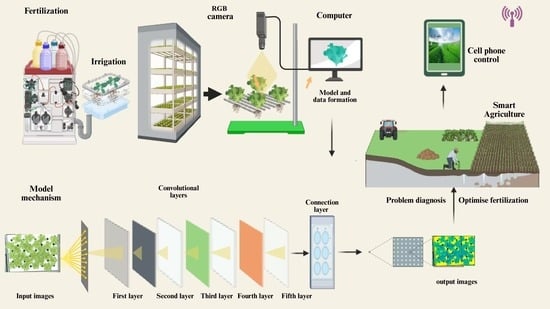
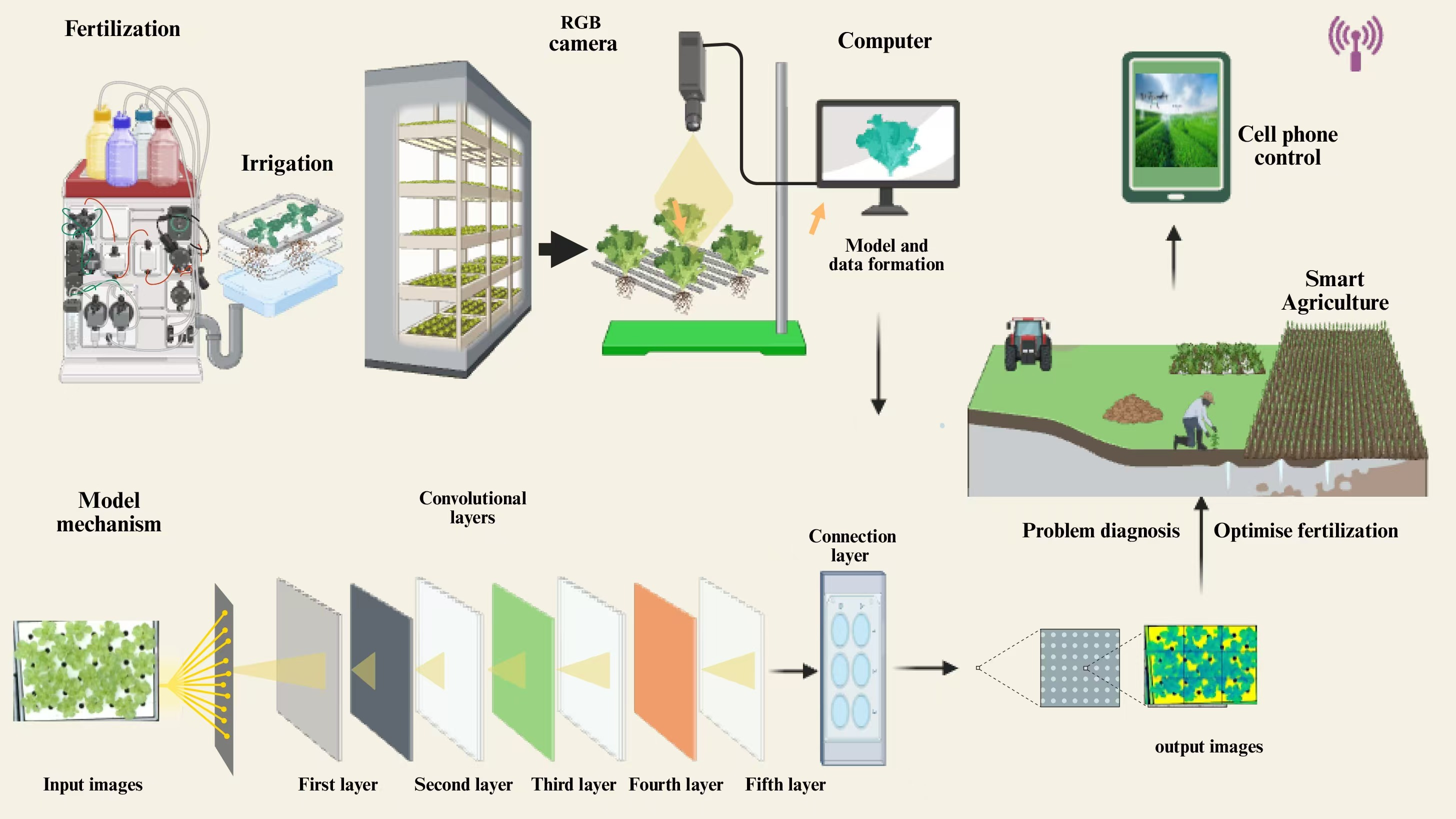
Graphical Abstract

1. Introduction

Climate change and rising world population increase pressure on agricultural production, which subsequently reduces arable lands, water sources, and biodiversity. Therefore, alternative crop production methods are gaining more and more interest and popularity [1]. In recent years, soilless growing techniques such as hydroponics and aeroponics have gained popularity in many countries [2]. This makes hydroponics particularly valuable for vertical agriculture and regions where there is poor soil quality or a water shortage [3]. Moreover, it is important to provide plants with essential nutrients and growing conditions (pH, temperature, and humidity). Although plants obtain ions at low concentration when continuously supplied, a change in equilibrium can cause plant toxicity [4,5].
Lettuce (Lactuca sativa L.) is a major leafy vegetable and contains many nutritional compounds (e.g., vitamins, minerals, phenolic compounds) that are part of a healthy diet, with a production of 27.5 Mt and a cultivation area of 1 Mha [6,7]. It is a widely produced and consumed leafy vegetable all over the world, China being the largest producer, followed by the US and Western Europe [8,9]. The nitrogen content in lettuce is an important reference indicator and plays a crucial role in development, significantly influencing the synthesis of amino acids, proteins, and chlorophyll contents in lettuce throughout its growth [10]. The application of nitrogen fertilizers significantly enhances crop yields. However, the current approach to nitrogen fertilizer application primarily relies on human judgment. Farmers frequently overapply nitrogen fertilizers in an attempt to increase yields, which can have unforeseen repercussions like reduced crop yields, environmental degradation, and a waste of resources. Therefore, it is crucial to accurately determine unique nitrogen conditions. This precision not only makes it possible to apply the right amount of nitrogen fertilizer, but it also helps to boost yields and cost savings [11]. Accurate nitrogen content estimation in lettuce enables optimized fertilization and improved crop quality and yield, supporting resource-efficient production and enhancing food security [3,12]. Traditional nitrogen detection techniques are mostly destructive biochemical detection methods. However, these methods require destructive sampling, which is expensive and time-consuming. As a result, there is a dire need for intelligent diagnostic tools that allow farmers to rapidly determine the nitrogen levels in lettuce plants without using destructive techniques [13,14].
As science and technology have advanced, optical imaging equipment has become widely available in daily life, providing a quick and easy way to take optical images. Plant nutrient levels can be quickly acquired by utilizing spectral imaging in conjunction with computer vision technologies. This method has the advantages of being quick, highly automated, and non-destructive [15]. In addition, machine learning techniques have been widely used in agriculture. For instance, Buxbaum [16] et al. verified the feasibility of using deep learning and RGB images to monitor the growth dynamics at the scale of individual plants under non-idealized planting conditions. Nowadays, non-destructive testing of crop characterization information extraction has been widely applied in predicting the composition of agricultural products and it has great potential in measuring the N content of lettuce [17,18].
Convolutional Neural Networks (CNNs) have become a fundamental tool in agricultural applications. Researchers have notably applied CNNs for diagnosing nutrient transportation and predicting yields in various agricultural products, including fruits and vegetables [19,20]. CNNs have opened up new possibilities for recognising nutrient deficiencies in crop nutritional status. For instance, Yu H et al. [21] utilized deep learning technology to extract features from lettuce phenotypes, achieving precise segmentation of the lettuce canopy in black screens. This achievement indicates that neural networks have a strong ability to extract features from RGB images of potted lettuce canopies. Moreover, OJOMO et al. [22] employed the bileNetv2 integrated into the DeepLabv3+ network and successfully achieved semantic segmentation of RGB visible-light images from the top-down perspective of the lettuce canopy with an accuracy of up to 0.9985. In addition, RGB images have a strong correlation with plant nutrition and are highly stable against environmental changes. Similarly, Yu et al. [23] developed two end-to-end deep learning models based on a two-dimensional convolutional neural network and a fully connected neural network for hyperspectral images of lettuce canopies, which directly predicted two tissue quality traits of lettuce—soluble solids content and tissue pH (both measured from lettuce juice as biochemical indicators of taste and harvest timing)—with prediction R2 values of 0.9030 and 0.8490, respectively.
The main way deep learning technology is applied in agriculture is by using deep convolutional neural networks to extract feature information, mainly for regression and classification [24]. This study mainly utilizes the regression application of deep learning, involving the neighborhood related to crop yield prediction. The common approach has shifted from directly using classical convolutional neural networks to adaptively modifying and reengineering their network structures to improve model accuracy [25]. For instance, Thaknetr et al. [26] built an improved lightweight VGG model—VGG-ICNN—which performed well on the public dataset of crop diseases. A stacking integrated convolutional neural network model was developed to determine the nitrogen nutrient levels in rice [26]. The authors obtained an ideal diagnostic accuracy of 96.41% using DenseNet121, ResNet50, and Inception ResNet V2 as base learners. With DenseNet121, the accuracy rose to 98.10% following the stacking algorithm’s integration of various models [27]. These integrative approaches demonstrate how well different models may be combined to improve crop nutritional status diagnosis accuracy while negotiating the difficulties of different nutrient levels and deficiency kinds in agricultural settings.
Prior work has introduced attention mechanisms into residual CNNs [28,29] and attention-gated or attention-enhanced encoder–decoder designs [30,31] In lettuce nutrient estimation, Cohen et al. compared ResNet- and Vision Transformer-based models using hyperspectral imagery [32]. Ensemble-learning approaches have also been used for crop nutrient monitoring [33], while residual networks incorporating multi-head attention have been reported in general image-classification research [34]. Agricultural Vision Transformer studies have employed image-based or spatial–temporal transformer pipelines for crop-yield prediction [35,36]. Recent lettuce research has evaluated EfficientNetV2-S for RGB-based nitrogen regression [37]. More general computer-vision studies include attention-augmented convolution [38], Bottleneck Transformer architectures that replace selected ResNet convolutions with self-attention [39], and the standard Vision Transformer, which processes projected image patches and uses a learnable classification token [40]. Accordingly, this study does not claim to be the first to combine MSA and ResNet, nor does it claim novelty for self-attention itself. The specific architectural question examined here is whether the integration mode and insertion depth of an MSA block affect tray-level multi-output nutrient regression when all models are evaluated under the same controlled image-acquisition setting. The proposed comparison considers two integration modes. The R-series retains the corresponding ResNet stage and laterally fuses an attention-enhanced representation, whereas the E-series replaces a selected ResNet stage with the SA block. Each strategy is evaluated at three depths. Unlike the standard ViT architecture [40], the attention input in the present framework is derived from an intermediate CNN feature map rather than directly from projected image patches, and no image-level classification token is used.
The objective was therefore to evaluate a controlled-condition proof-of-concept framework for mapping one standardized tray-level RGB image to a jointly predicted N–P–K nutrient-status vector. The controlled setting reduces variation unrelated to the architectural comparison, but it does not establish external validity.
The contributions of this study can be summarized as follows:
  • A systematic evaluation of two strategies for integrating multi-head self-attention into a ResNet50 backbone—lateral fusion (R-series) and stage replacement (E-series)—for non-destructive lettuce nutrient diagnosis from canopy RGB imagery.
  • A comparison of three attention insertion depths per strategy, yielding six ResNet50-SA variants for tray-level, multi-output estimation of lettuce N, P, and K status, matching the management unit of greenhouse fertigation.
  • A batch-grouped five-fold cross-validation against five baseline CNN architectures, reflecting batch-to-batch variation under production conditions, together with explicit boundaries on statistical inference, nutrient-specific interpretation, and external agricultural application.

2. Materials and Methods

2.1. Sample Collection and Data Acquisition

The experiment used the commercially available lettuce cultivation variety “Premium Italian lettuce (Lactuca sativa L. var. Ramosa Hort.)” purchased from the Beijing APEX Agriculture Company. The experiment was conducted from May 2023 to June 2023 using floating soilless cultivation in the Songjiang District greenhouse of Dogilead Agricultural Technology (Shanghai) Co., Ltd. Seedling tray size: 80 cm (bottom diameter) × 60 cm (width) × 10 cm (height); substrate: a mixture of coir, vermiculite, peat, and perlite. The nutrient solution for the experiment was a commercially available water-soluble fertilizer product (water-soluble fertilizer 20-20-20, Stanley Agri-Group, potassium nitrate type, N + P2O5 + K2O ≥ 60%), diluted 500 times, and then water was added to adjust the EC value to 2.0 mS/cm. Spray once every 5–7 days. A total of 96 trays were planted, with 24 plants in each pot, totalling 2304 plants. The physiological attributes and elements of lettuce growth were measured by sampling every two days, and the sampling time was fixed between 9 a.m. and 10 a.m. A total of 16 batches were sampled, with 6 trays taken each time, 5 plants in each tray, and 30 individual plants in each batch, totalling 480 plants. Each image is paired with one N-P-K vector calculated from destructive measurements of five plants in that tray. The contents of nitrogen, phosphorus, and potassium in lettuce were tested by the Analysis and Testing Center of Nanjing Agricultural University. Model training was conducted on a workstation equipped with an NVIDIA GeForce RTX 4090 GPU (NVIDIA Corporation, Santa Clara, CA, USA) with 24 GB graphics memory, a 13th Gen Intel Core i5-13600KF CPU (Intel Corporation, Santa Clara, CA, USA) at 3.50 GHz, and 32 GB system RAM, under a 64-bit Windows (v11) environment.

2.2. Image Acquisition and Dataset Building

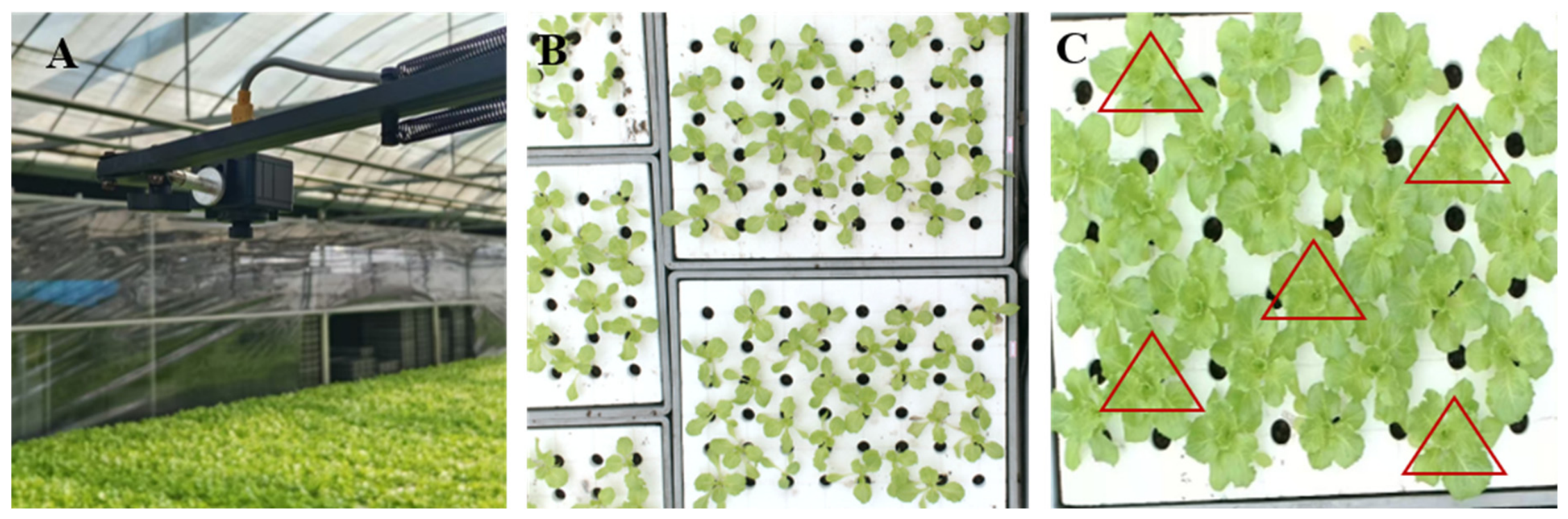
This study implemented a detailed image pre-processing workflow to enhance the quality and consistency of lettuce images under control condition [32]. Image acquisition was carried out in the greenhouse of the Doligid Company, using the Savage HD-X12MP-AF model camera to capture high-definition photos of lettuce cultivation trays with a top-down view resolution of 3840 × 2880. We selected a total of 96 groups of lettuce for the dataset, each photo covering two complete cultivation trays, and through meticulous cropping, we separated the images of the two cultivation trays from each photo, resulting in 96 separate images of lettuce cultivation trays. Before model input, each cropped tray image was resized to 224 × 224 pixels, converted to a 32-bit floating-point array, and scaled from [0, 255] to [0, 1] by dividing each RGB value by 255.0. No additional channel-wise mean subtraction or standard-deviation normalization was applied. No geometric or color-based data augmentation was used. Because the task was formulated as tray-level regression, no nutrient-category, region, or bounding-box annotation was performed; supervision was provided solely by the tray-level N–P–K target vector derived from destructive laboratory measurements, and no image-level manual annotation was required.
After quality control, we sampled the lettuce plants at fixed positions within the cultivation plates, selecting five different plants from each cultivation plate for sampling (Figure 1 and Figure 2B). By collecting the above-ground parts of these plants, we tested their total nitrogen, total phosphorus, and total potassium content. To ensure representativeness of the data, the average values of nitrogen, phosphorus, and potassium in each tray of five lettuce plants were calculated as three-dimensional label values for the corresponding tray photos. The 96 original images were divided into training sets, test sets, and validation sets in a ratio of 76:10:10 for model training and evaluation.

2.3. Grouped Five-Fold Cross-Validation and Statistical Analysis

The 96 tray images were grouped by sampling batch (16 batches, 6 trays per batch; Section 2.1), and a five-fold group cross-validation scheme was applied. The 16 batches were divided into five fold groups of 4, 3, 3, 3, and 3 batches, so that the test folds contained 24, 18, 18, 18, and 18 tray images, respectively. In each iteration, one fold group served as the test set and the remaining four fold groups were used for training; the five test folds are mutually exclusive at the batch level, ensuring that trays from the same acquisition batch never appeared in both the training and test sets of any fold, thereby preventing batch-level data leakage. Within each training portion, a subset of trays was held out as a validation set for early stopping and hyperparameter selection; test folds were never used for model selection. No data augmentation was applied. Model performance was measured by R2, RMSE, and MAE (Section 3.5), macro-averaged across N, P, and K, and is reported as mean ± standard deviation across the five folds. Per-fold results for all models are provided in Table 2.
For statistical comparison between ResNet50_SA_RV1 and each baseline model, the out-of-fold predictions from all five folds were pooled, yielding 96 paired predictions per model (one per tray image). The difference in macro-averaged MAE (ΔMAE) between ResNet50_SA_RV1 and each baseline was quantified on this paired image-level sample. Ninety-five percent confidence intervals were estimated using a percentile bootstrap with 5000 resamples (random seed 42), and statistical significance was assessed with a paired permutation test (5000 permutations, random seed 42). The resulting p-values were adjusted for multiple comparisons across all RV1-versus-baseline tests using the Holm–Bonferroni method (family-wise significance level 0.05).

3. Construction of Deep Learning Algorithms

3.1. Design of ResNET-SA Network Structure Based on ResNet

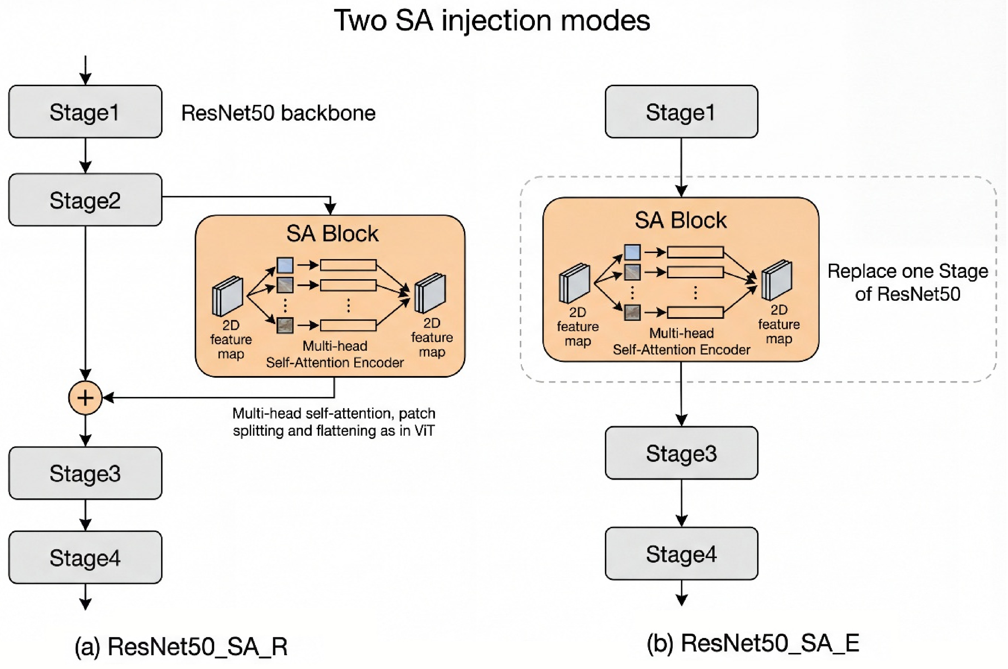
Two self-attention blocks (SA blocks) are proposed in this paper. The first one applies the output of the SA block as additional information to the original output feature map of the Stage in ResNet50; The second option is to replace the Stage in the ResNet50 with the SA block, that is, the SA block becomes a section of the supporting structure of the ResNet50, and the feature map goes in and out of the SA with attention information and enters the lower layer (Figure 3). The multi-head is derived from the Attention Block in the Transformer model [21], and the feature map is segmented by referring to the method of image segmentation in ViT [22], flattened and passed into the encoder in the form of simulated word vectors The encoding matrix with attention scores output by the feedforward neural network of the encoder is then restored to a two-dimensional feature map as the input for the next layer.
In other words, the two options constitute a lateral-fusion strategy (R-series) and a stage-replacement strategy (E-series): in the R-series, the original ResNet stage is retained, and the attention-processed representation is fused as additional information, whereas in the E-series, a selected ResNet stage is replaced by an SA block. In both cases, the SA input originates from an intermediate CNN feature map: the feature map is converted to a token sequence, processed by the self-attention encoder, reshaped to a two-dimensional feature map, and passed to the remaining convolutional hierarchy. The model therefore differs from a standard ViT, which tokenizes image patches directly and commonly uses an image-level class token.

3.2. Activation Function ReLU

ReLU is a commonly used activation function that can transform the nonlinear relationship of the input into a linear relationship, thereby increasing the nonlinearity of the neural network. The ReLU function is characterized by directly outputting the value when the input is greater than 0 and outputting 0 when the input value is less than or equal to 0. This characteristic gives the ReLU function features such as unilateral suppression, a relatively wide excitation boundary, and sparse activation. Its mathematical expression is as follows:
ReLU ( x )   =   max ( 0 ,   x )
Here, x is the input of the neuron. The ReLU function is widely used in neural networks. It can effectively alleviate the vanishing gradient problem, accelerate the convergence speed of the model, and improve the generalization ability of the model.

3.3. Optimizers and the Loss Function

In model training, we used the Mean Squared Error (MSE) as the loss function to measure the gap between the model’s predicted values and the true values. Its mathematical expression is as follows:
MSELoss   =   1 n i = 1 n y i y i ^ 2
Here, n is the sample size, y i is the real label, and y i ^ is the label predicted by the model.
In the optimization process, we used Stochastic Gradient Descent (SGD) as the optimizer. The parameter update rule is:
θ t + 1 = θ t η J ( θ t )
Here, θ t is the parameter vector, and η is LR, J ( θ t ) is the gradient of the loss function with respect to the   θ t parameter.

3.4. Model Evaluation Methods

When evaluating model performance, we used the following metrics: R2 (R Square), Root Mean Squared Error (RMSE), and Mean Absolute Error (MAE). They are defined as follows:
R 2 = 1 i = 1 n ( y i y ^ i ) 2 i = 1 n ( y i y ¯ ) 2
RMSE = 1 n i = 1 n ( y i y ^ i ) 2
MAE = 1 n i = 1 n y i y ^ i
Here, y i is the true value, y ^ i is the model predicted value, and y ¯ is the average of the true values.

3.5. Encoder Structure Design with Improvements and Adaptations to ResNet50_SA_RV1

3.5.1. Embedded Feature Map Embedding

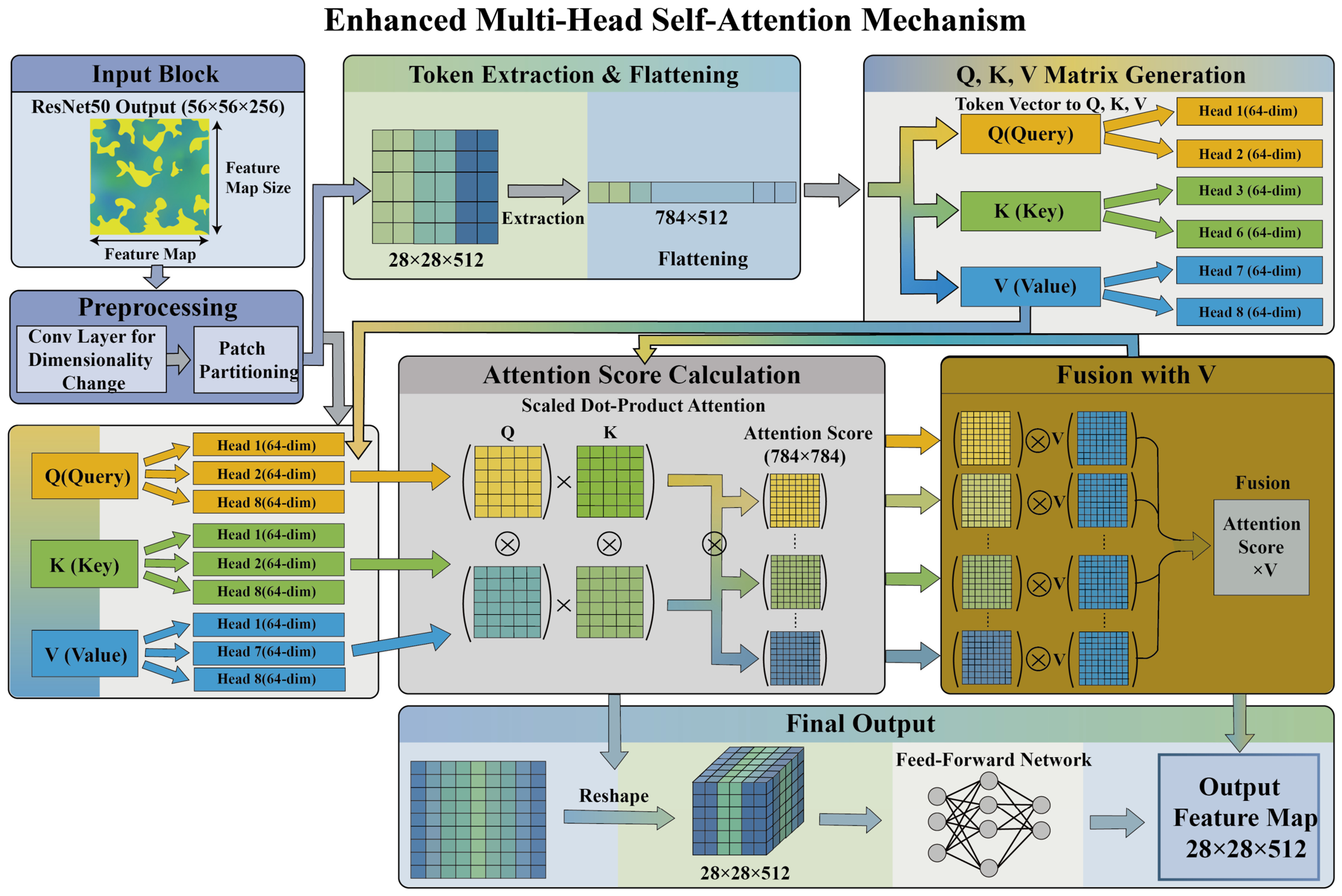
This layer is the preprocessing of the feature map, and the receptive field size of the attention is determined at this layer. The 56 × 56 (256-channel) feature map is first transformed into a 28 × 28 (512-channel) patch puzzle through a convolutional layer, which defines the size of the attention receptive field for the entire SA block as feature extraction for the original image input, with 256 and 512 being the input dimension and output dimension of the SA block, respectively. The purpose of this setup is to keep the size of the Stage block at that level position in the ResNet50 original network consistent in and out, and finally to flatten it to 784 × 512 to become the token vector required for the attention input.

3.5.2. Encoder Self-Attention Encoding

This layer is designed to quantify the relationships between 28 × 28 modules (i.e., 784 positions) by calculating attention by establishing a Q (query vector), K (key vector), and V (value vector) matrix. First, a 784 × 512 token vector is obtained from the upper layer, and then three “clones” are generated through a fully connected layer, namely three vectors of length 784, named query vector Q, key vector K, and value vector V, respectively. Then, these vectors are split into multiple heads (num_head = 8) in the channel dimension, resulting in an output of 3 × 8 × 784 × 64.
Next, the attention score matrix is calculated by performing matrix multiplication on 64 channels × Q, K, that is, on the last two dimensions of the above output, to calculate the attention score, resulting in an 8 × 784 × 784 attention score matrix. Matrix multiplication is performed on the 8 784 × 64 value matrices formed by the score matrix and the V vector on the 64 channels, and the 8 × 64 channels of the 8 head divisions are concat merged, and the attention score is reflected on the 784 × 512 feature map. Finally, the feature map is given a nonlinear activation map through the feedforward network MLP, which goes directly to the next identical encoder for attention encoding again (where depth = 12 goes into 12 encoders), if the last attention encoding is completed, After the output, the feature map is restored to a two-dimensional 512-channel 28 × 28 × 512 feature map with information from 12 attention encodings, which is used to form the input for the next Stage of ResNet.
It is worth noting that in the ViT model with a similar approach to this paper, before the Q, K, and V matrices are built, an additional dimension is added to the token to serve as the vector for the subsequent one-hot output of classification, and sometimes position encoding is added to the token vector. We believe that these treatments are not suitable for the task of this paper and do not adopt them.
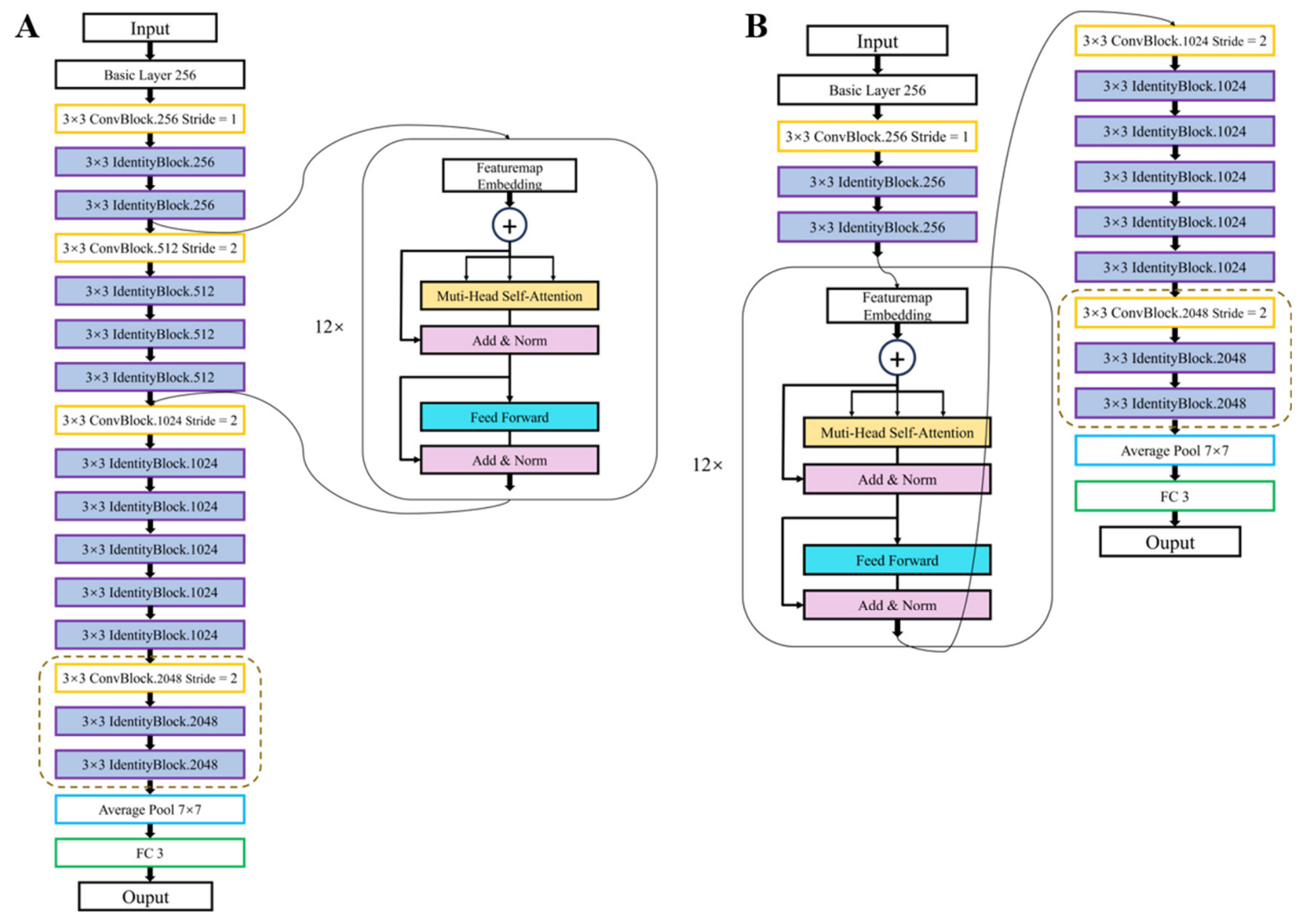
ResNet_SA is a fusion innovation network based on ResNet50 and with SA block as an important optimization tool. First, we use ResNet as the underlying framework, which includes the basic layer, the fully connected layer, and four stages. A 224 × 224 × 3 RGB image goes into the basic layer and is downsampled to a 56 × 56 × 64 feature map by a convolutional layer with a kernel size of 7 × 7 and a step size of 2, and then enters the four stages. Each Stage consists of several Residual blocks, with the number of residual blocks in stages 1 to 4 being 3, 4, 6, and 3, respectively. Each time through a Stage, the feature map is downsampled to size 1 of the input of that block, and the number of channels is doubled. The first residual Block in each Stage will be different from the subsequent ones. These two residual blocks are named Conv Block and Identity Block, respectively. The convolution block contains three convolutional layers. The first convolutional layer undergoes downsampling, followed by a BN layer and the ReLU activation function. Each of the latter two convolutional layers performs a BN operation. Finally, a shortcut is performed before the output, that is, the initial input of the convolutional block is convolved once and then added to the feature map output by the three convolutional layers. The identity block is structurally similar to the convolutional block, except that the second convolutional layer has an additional ReLU activation function, which adds the input and output results directly without convolution during residual connection (Figure 4).
In the ResNet50_SA_E series, SA replaces one of the original Stages of ResNet50 as part of the backbone structure, and V1 to V3 are the SA blocks replacing Stages 2, 3, and 4, respectively. The design was intended to explore the impact of using the MSA mechanism to process feature maps of different receptive fields on the overall accuracy of the model. For example, the SA feature map input size in ResNet50_SA_EV1 is 56 × 56, which yields more detailed attention information compared to the 14 × 14 in ResNet50_SA_EV3. This principle is similar to how the human eye recognizes images. High-resolution images tend to draw more attention to details, while blurry images or those in the line of sight are extremely difficult to extract detail information from.
For a clear demonstration of the structure, two V1 versions of the series model structure are presented here. The specific implementation of ResNet50_SA_RV1 is shown in Figure 5A, and the specific implementation of ResNet50_SA_EV1 is shown in Figure 5B. The two Figures, respectively, show the methods of side connection and internal embedding of the encoder.

4. Experimental Results

4.1. Feature Information Propagation

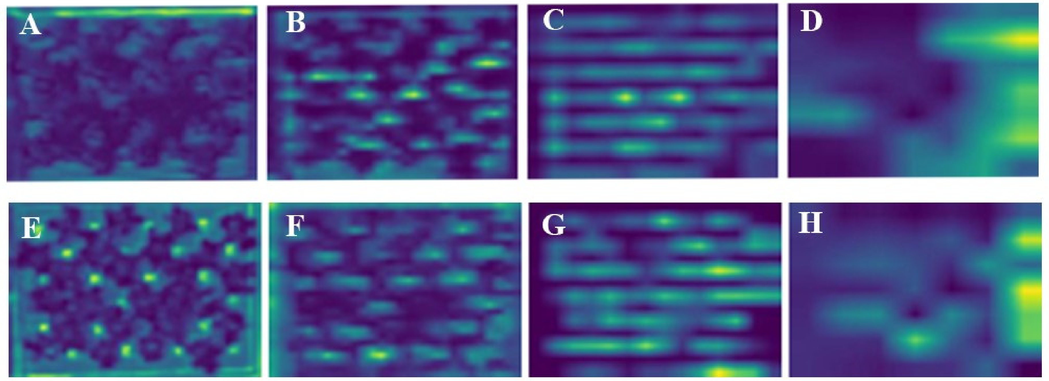
When delving into the differences between the ResNet50 and ResNet50_SA_RV1 models in terms of lettuce feature extraction and propagation, we analyzed the feature-map outputs of each model during image processing, which were reconstructed from the original image in Figure 2B using the trained test model. As can be seen from the comparison of feature maps in Figure 6, (H) shows more high-lighted regions and attention points compared with (D) for the same lettuce image, where RV1 exhibits higher sensitivity for capturing lettuce canopies. The feature maps (Figure 7) represent intermediate activations generated during hierarchical feature extraction. They were visualized to qualitatively compare how different MSA insertion strategies affected spatial feature representation, activation distribution, and information propagation within the ResNet hierarchy.
ResNet50, as a classic CNN architecture, effectively mitigated the potential performance degradation of deep networks during training by introducing residual connections. As the depth of the network increases, from the basic layer to higher levels (layer1 to layer4), the degree of abstraction of the feature map gradually increases, from capturing the bottom edge and texture information of the image to extracting more advanced semantic features.
In contrast, the core improvement of ResNet50_SA_RV1, as a variant of ResNet50, lies in the introduction of MSA mechanisms. The MSA mechanism gives the model greater flexibility and targeting in feature extraction, enabling it to focus more effectively on key areas in the image, thereby enhancing the model’s representational and generalization capabilities. By comparing the feature map outputs of the two models at the same level (Figure 7), we find the following:

4.1.1. Semantic Information Extraction

At the lower levels of the network, such as layer1, the feature map of ResNet50_SA_RV1 retains more detailed information about the lettuce canopy compared to ResNet50, and performs significantly better than ResNet50 in distinguishing the texture of the lettuce leaf edge from the background. This is mainly due to the MSA mechanism’s precise localization and emphasis on key areas of the image. The feature map of ResNet50 is likely to be relatively blurry. As the network hierarchy deepened, both models gradually demonstrated the ability to capture advanced semantic information about the texture and color of individual leaves of lettuce. However, ResNet50_SA_RV1 performed more precisely and comprehensively in extracting semantic information through the self-MSA mechanism, which helped the model better understand the context in the image.

4.1.2. Robustness

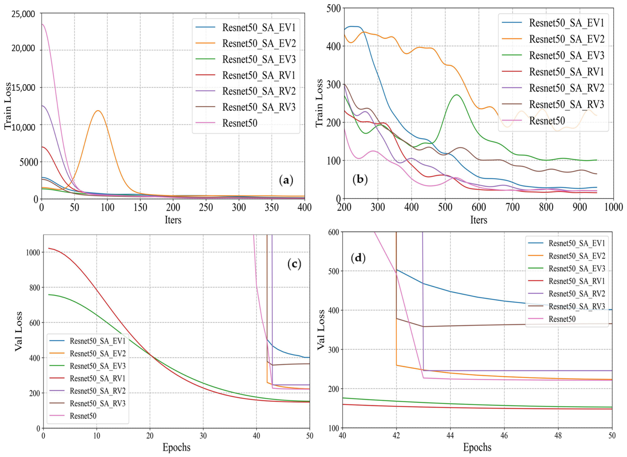
In terms of robustness, because the dataset is single, the dataset images are set in terms of light intensity, color saturation, shooting angle, and lettuce variety in accordance with the principle of fit for the lettuce production scenario application, which means that the feature extraction effect is highly specific and not robust. In summary, ResNet50_SA_RV1 shows significant advantages in feature extraction and propagation by integrating the MSA mechanism on top of ResNet50. However, further experimental verification is needed to verify the actual performance of these advantages in specific tasks. The performance evaluation of a model often relies on its performance on both the training set and the validation set. By analyzing the downtrend of train loss and validation loss, we can gain a deeper understanding of the differences in feature learning and generalization ability among different models. In this study, we compared the characteristics of ResNet50 and its variants with different self-attention (SA) modules, such as EV1, EV2, RV1, etc., during the loss degradation process, aiming to reveal the superiority or inferiority of these models in terms of performance.
First, from the perspective of training loss, all models show a rapid drop in loss in the early stages of training, which is a natural phenomenon for models in learning the underlying features of the data. Notably, ResNet50_SA and its variants with SA blocks showed similar loss reduction trends during training, but in the later stages of training, the models with SA blocks (such as EV1, EV2, RV1, etc.) showed more stable loss values. This trend suggests that these models may have captured the complex features of the data better and have moderate robustness against overfitting. However, ResNet50_SA_RV3 saw an increase in loss values in the later stages of training, possibly due to the model’s excessive complexity leading to overfitting on the training set.
Secondly, the change in validation loss provides us with clues about the generalization ability of the model on unseen data. Compared with the training loss, the decline rate of the validation loss may be slower and may be accompanied by fluctuations, which reflects the challenges the model faces when adapting to new data. On the validation set, ResNet50_SA and its variants with SA blocks also show a similar trend, but models with SA blocks typically have lower validation loss values. This finding further confirms the effectiveness of the MSA mechanism in improving model performance.
Overall, variants of ResNet50 with SA blocks showed more stable and lower loss values during the loss reduction process, suggesting an advantage in feature learning and generalization ability. However, excessive model complexity can lead to overfitting problems, so it is necessary to weigh the complexity and performance of the model when choosing a model to achieve the best results in practical applications.

4.2. Model Performance

As can be seen from the model test results (Table 1), we compared the performance of different models on the validation set and the test set, with the main metrics being R2, RMSE, and MAE. First, we can note that on the validation set, the R2 of the ResNet50_SA_RV1 model reached 0.89, which is much higher than that of other models, while the RMSE and MAE were relatively low. This indicates that the model has a stronger predictive ability on the validation set and is more accurate than other models. On the test set, the ResNet50_SA_RV1 model also performed well, with R2 reaching 0.92 and RMSE and MAE showing more stable loss values than EV1, EV2, RV1, etc. This trend suggests that these models may have captured the complex features of the data better and have moderate robustness against overfitting.
Secondly, the variation in validation loss provides us with clues about the model’s ability to generalize on unseen data. Compared with the training loss, the decline rate of the validation loss may be slower and may be accompanied by fluctuations, which reflects the challenges the model faces when adapting to new data. On the validation set, ResNet50_SA and its variants with SA blocks also show a similar trend, but models with SA blocks typically have lower validation loss values. This finding further confirms the effectiveness of the MSA mechanism in improving model performance.
Overall, variants of ResNet50 with SA blocks showed greater stability and lower loss reduction, further verifying the robustness of the model.
The ResNet50_SA_RV1 model, which has a relatively small number of parameters, 62.8 M, but performs relatively well on both the validation set and the test set, possibly because it uses the MSA mechanism to improve ResNet50 and enhance the model’s feature extraction ability. In contrast, the ResNet50_SA_EV3 model performed relatively poorly on the validation set and test set, despite having a large number of parameters, reaching 623.4 M, but with a lower R2 and higher RMSE and MAE. This may be because in this model, the application of the MSA mechanism did not effectively improve the model’s performance; instead, it may have increased the model’s complexity, resulting in a decline in performance.
In addition, we can also observe that the computational cost (GFLOPS) of the ResNet50_SA_RV1 model is relatively low, at 17.065, while that of the ResNet50_SA_RV3 model is the highest, at 17.645. Although the ResNet50_SA_RV3 model has a higher R2 on the validation set, its large computational load may increase the training and inference time cost of the model. Therefore, in practical applications, both model performance and computational cost need to be taken into account (Figure 8).
In summary, the ResNet50_SA_RV1 model performs better than other models on validation sets and test sets, possibly due to its relatively simple structure and effective feature extraction capabilities. Other models may have performed poorly due to higher model complexity or improper application of the MSA mechanism. When choosing a model, one needs to take into account the model’s performance, computational cost, and application scenarios in light of the actual situation. These results, however, were obtained on a single fixed partition; their robustness is further examined through grouped cross-validation in Section 4.3.
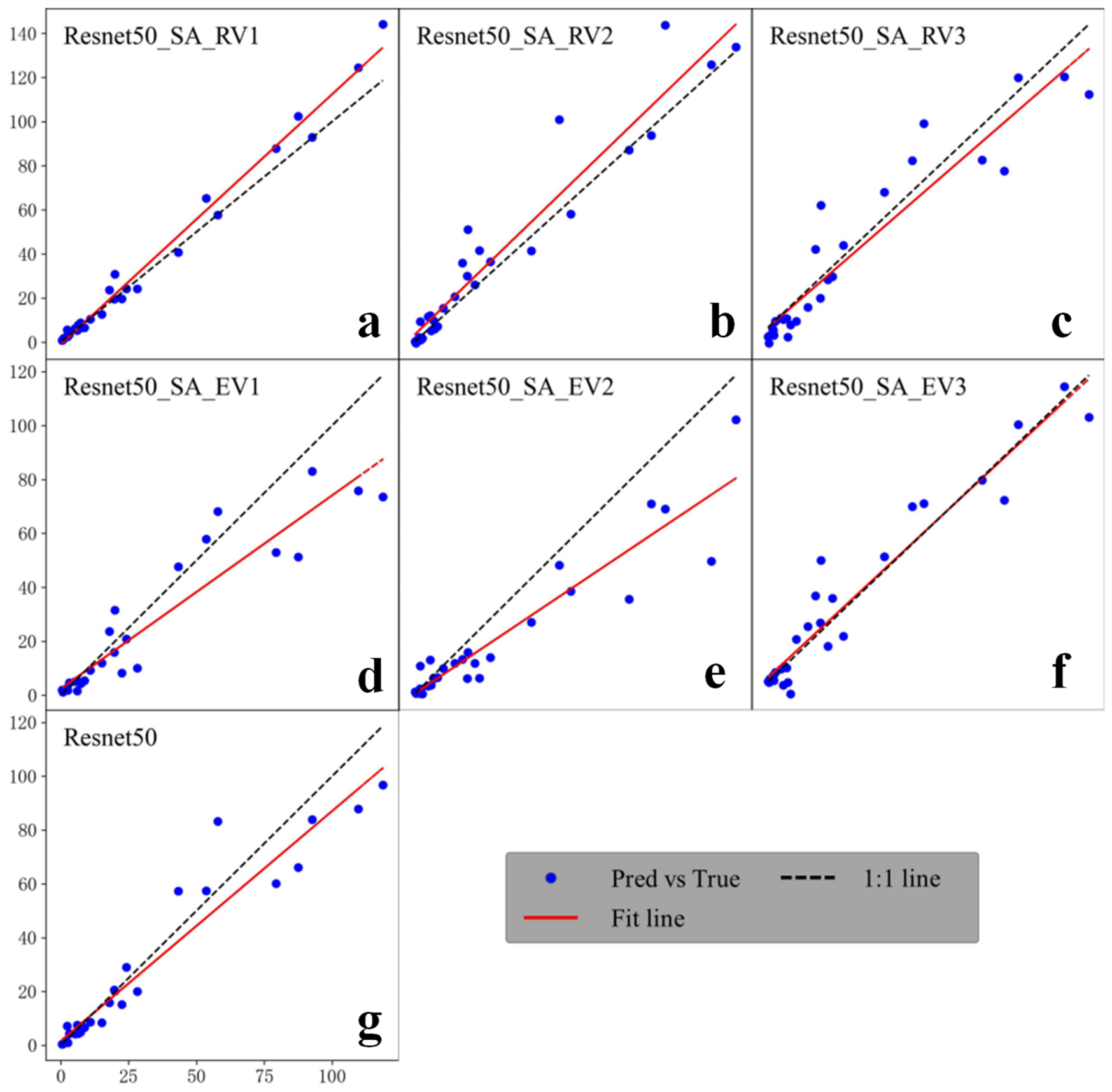
As illustrated in Figure 7, the SA-enhanced ResNet50 model we proposed demonstrates exceptional prediction consistency across the three random validation sets (RV1–RV3). The blue scatter points are tightly aligned with the 1:1 baseline, and the red fitted line nearly overlaps with the ideal line, indicating that the enhancement module effectively mitigates prediction bias. For the external validation sets (EV1–EV3), despite slight scattering of the points, a strong positive correlation is still maintained overall, which confirms the model’s reliable cross-distribution generalization capability. In comparison with the performance of the vanilla ResNet50, the SA-enhanced variant exhibits a denser distribution of scatter points and a fitted line that is more closely aligned with the baseline—findings that further validate the efficacy of the proposed enhancement strategy in improving the stability and accuracy of model predictions.
The purpose of this study was to evaluate an architectural hypothesis under controlled acquisition conditions: whether applying multi-head self-attention to intermediate ResNet50 feature representations could improve joint tray-level N–P–K regression. The controlled environment reduced variation unrelated to the architectural comparison and allowed the effects of alternative feature-extraction strategies to be examined under a common image-acquisition setting. Comparisons with ResNet18, SqueezeNet1.1, ShuffleNetV2, and RegNet were added to assess whether the observed performance extended beyond comparisons among ResNet50 variants. These experiments provide preliminary evidence of algorithmic feasibility for controlled-condition biological image regression but do not establish sensitivity to all subtle nutrient variations or robustness across seasons, cultivars, locations, or field environments.

4.3. Grouped Five-Fold Cross-Validation and Benchmark Comparison

To verify that the superiority of ResNet50_SA_RV1 is not an artifact of a particular data split, grouped five-fold cross-validation was conducted for ResNet50_SA_RV1, the ResNet50 baseline, and four conventional CNN architectures of different scales (ResNet18, SqueezeNet1_1, ShuffleNetV2, and RegNet), as summarized in Table 2. Notably, the five-fold mean R2 values of ResNet50_SA_RV1 and ResNet50 (0.92 and 0.81, respectively) coincide with the fixed-split test results in Table 1, indicating that the original partition did not overstate model performance.
The proposed ResNet50_SA_RV1 achieved the highest accuracy (R2 = 0.92 ± 0.03; RMSE = 7.16 ± 1.77 mg/g; MAE = 4.06 ± 1.58 mg/g), clearly outperforming the ResNet50 baseline (R2 = 0.81 ± 0.06; RMSE = 9.91 ± 1.96 mg/g; MAE = 6.31 ± 1.54 mg/g). Paired bootstrap analysis tentatively verified that the stability of this improvement was statistically significant, with a ΔMAE of −2.25 mg/g (95% CI: −2.88 to −1.62) and a Holm-adjusted p-value < 0.001. Among the conventional baselines, ResNet18 achieved the closest performance to ResNet50 (R2 = 0.80 ± 0.06) despite its substantially smaller parameter count, while SqueezeNet1_1, ShuffleNetV2, and RegNet yielded progressively lower accuracy (R2 range: 0.49–0.75), confirming that the performance gain of ResNet50_SA_RV1 stems from the attention mechanism rather than increased model capacity alone.

5. Discussion

This work integrates the multi-head self-attention (MSA) mechanism into the residual neural convolutional network (ResNet-SA), which was designed by collecting environmental data through high-definition RGB images, aiming for high-precision diagnosis of lettuce nitrogen levels.

5.1. Model Architecture Comparison and Innovation

Wang et al. proposed a network with residual connections between soft attention modules, which performed well on the CIFAR10 dataset [33]. Previous studies have improved the attention mechanism of ResNet, such as using the soft attention mechanism to implement the segmentation task on private datasets using a compressed attention encoder and a multi-head attention decoder [29,30]. As these studies show, attention-enhanced CNNs and CNN–Transformer hybrids have been reported previously [31]. The contribution of this study is therefore not a first combination of MSA and ResNet, but a systematic comparison of two integration modes—lateral fusion and stage replacement—at three insertion depths for tray-level multi-output nutrient regression. A recent paper proposed embedding a multi-head attention mechanism encoder (Trans SE-ResNet) at the end of the ResNet structure for pneumonia diagnosis in chest CT images, achieving extremely high accuracy in pathological classification tasks [31]. Compared with these studies on natural-image benchmarks and medical diagnosis, the present method targets high-precision estimation of crop nitrogen, phosphorus, and potassium levels [34]. Li et al. [39] reported a test-set R2 of 0.9859 for lettuce nitrogen estimation from RGB images using EfficientNetV2-S; it should be emphasized, however, that their prediction was performed at the single-plant scale—each image contained one lettuce plant, and the model was developed on 4620 such single-plant images expanded by data augmentation, Meanwhile, Cohen et al. [32] reported a test R2 of 0.65 for nitrogen using raw hyperspectral imagery. These results cannot be treated as a leaderboard because the experimental units, nutrient ranges, modalities, and validation protocols differ. The distinct objective here is joint tray-level estimation of N, P, and K from a single low-cost RGB view. We created three improved models of SA blocks for ResNet50 and optimal position for attention embedding, and identified the best-performing of six model variants -ResNet50_SA_RV1. RV1 produced the highest test-set R2 point estimate among the ResNet50-based variants; however, a single split cannot establish a stable architectural ranking, so this result is interpreted as preliminary evidence that integration mode and insertion depth matter. Compared to feature maps being used for feature extraction and propagation in ResNet50 and ResNet50_SA_RV1, we found that the introduction of the MSA mechanism significantly enhanced the model’s ability in feature extraction and propagation. ResNet50_SA_RV1 not only retains more detailed information at a lower network level but also extracts advanced semantic information more precisely at a higher level, which helps the model better understand the context in the image [35].
Further, by analyzing the downtrend of training loss and validation loss, we found that the ResNet50 variant with SA block had a more stable loss during training and a lower validation loss, demonstrating the effectiveness of the MSA mechanism in improving the generalization ability of the model.

5.2. Model Performance Analysis

In order to verify the reliability and stability of our model, we compared the performance of different models on validation sets and test sets, mainly based on evaluation metrics including R2 (coefficient of determination), RMSE (root mean square error), and MAE (mean absolute error). These metrics provided us with an intuitive measure of the accuracy and robustness of the model’s predictions. The ResNet50_SA_RV1 model stands out particularly from the results of the validation set (Table 1). Its R2 value was as high as 0.89, significantly better than other models, while the values of RMSE and MAE were relatively low. This result indicates that the ResNet50_SA_RV1 model not only has a stronger predictive ability but also provides more accurate predictions.
The regression R2 of the multimodal ViT model incorporating the time dimension constructed by Lin et al. in a county-level yield prediction task for four crops, namely corn, cotton, soybean, and winter wheat, was at the levels of 0.7 and 0.8 [36]. Furthermore, an earlier study by Bi et al. [37] used the VIT model to predict soybean yields, with a regression prediction R2 of 0.664. On the test set, the ResNet50_SA_RV1 model demonstrated superior performance. Its R2 value rose further to 0.92, while RMSE and MAE values remained low. This performance further validates that the ResNet50_SA_RV1 model can achieve high prediction accuracy on small datasets after introducing an attention mechanism with a relatively large number of parameters.
Analyzing the characteristics of the ResNet50_SA_RV1 model in terms of model size, it has a relatively small number of parameters, only 62.8 M. In contrast, the ResNet50_SA_EV3 model performed relatively poorly on both the validation set and the test set. Despite having a large number of parameters, reaching 623.4 M, it performed poorly on three metrics: R2, RMSE, and MAE. This may be because, in the model, the MSA mechanism completely replaced the main structure of ResNet in Stage 3, which, on the one hand, caused the information propagation chain of ResNet itself to break, and on the other hand, the application of the MSA mechanism did not effectively improve the performance of the model. Instead, it may be due to the excessive complexity of the model, which led to performance degradation and overfitting. In addition, we also note that the ResNet50_SA_RV1 model has a lower computational effort (GFLOPS) of 17.065, which gives the model a lower time cost during training and inference. The ResNet50_SA_RV3 model had the highest computational cost at 17.645. Overall, the ResNet50_SA_RV1 model demonstrated excellent performance on both the validation set and the test set, mainly due to its relatively simple structure and effective feature extraction capabilities. In practical applications, we need to select the most suitable model based on specific scenarios and requirements, taking into account factors such as model performance, computational cost, and application scenarios.
The grouped cross-validation results (Section 4.3) provide important context for interpreting model performance. The five-fold mean R2 of 0.92 ± 0.03 for ResNet50_SA_RV1 demonstrates that the attention-based improvement is stable across independent batch groupings rather than an artifact of a favorable data split, which is further supported by the significant paired ΔMAE (95% CI: −2.88 to −1.62; Holm-adjusted p < 0.001). Notably, ResNet18 achieved an accuracy comparable to the deeper ResNet50 baseline (R2 = 0.80 vs. 0.81), suggesting that at this dataset scale (96 tray images), model depth alone does not guarantee performance gains—the attention mechanism, rather than capacity scaling, is the primary driver of improvement. Nevertheless, these estimates remain bounded by the single-season, single-cultivar experimental design; external validation across multiple growing seasons and commercial greenhouse conditions is required to establish generalizability. In addition, nitrogen, phosphorus, and potassium were represented as a unified three-dimensional target vector and learned simultaneously using a shared feature-extraction network. This multi-output design was intended to capture visual representations shared among nutrient-related canopy responses and to exploit potential relationships among the three nutrient targets. The reported MSE and R2 are aggregate multi-output metrics calculated for the complete N–P–K prediction vector and therefore represent the model’s overall nutrient-prediction performance.

5.3. Main Limitations of the Study and Corresponding Strategies

A dataset consisting of 96 RGB images of lettuce canopies was utilized in this study. Due to the limited sample size, the model struggles to generalize to rare nutrient conditions—such as severe potassium deficiency—that account for a small proportion of the dataset. Specifically developed for Italian premium loose-leaf lettuce, the model depends entirely on RGB images, which only capture visible light spectra. As a result, it faces inherent difficulties in identifying subtle nutrient variations that do not present obvious changes in color or texture. All images were acquired under controlled conditions of greenhouse floating-plate soilless cultivation, where lighting, shooting angles, lettuce varieties, and nutrient solution formulas remained constant. The high homogeneity of the dataset ultimately leads to insufficient environmental robustness of the model. Previous agricultural imaging studies have evaluated multi-target regression from standardized top-view lettuce images and proof-of-concept nutrient estimation from lettuce imagery using relatively limited datasets under controlled or semi-controlled acquisition conditions [38,39]. These studies provide methodological precedent for exploratory image-based regression but do not, by themselves, establish external generalizability. Because all candidate architectures in the present study were evaluated using the same observations, target definitions, and evaluation protocol, the results provide a preliminary internal comparison of model configurations. Nevertheless, limited sample sizes can produce substantial uncertainty in performance estimates and increase sensitivity to data partitioning [38] while insufficient dataset size and diversity may restrict model transfer across biological materials and imaging conditions [40]. Therefore, the reported performance should be interpreted as preliminary evidence under the acquisition conditions represented in this experiment, rather than as evidence of generalization across fields, cultivars, seasons, geographic regions, or imaging systems.
To address these limitations, future research will expand the dataset by incorporating images of open-field lettuce grown in different geographical regions, across various growing seasons, and of diverse varieties. Synthetic data augmentation techniques—including lighting adjustments, image rotation, and blurring—will be employed to simulate environmental noise encountered in actual agricultural production. A transfer learning approach will be adopted: ResNet50_SA_RV1 will first be pre-trained on large public agricultural image datasets like PlantVillage, followed by fine-tuning using lettuce nutrient data to enhance its ability to generalize features. Additionally, a lightweight crop-specific feature adaptation layer will be integrated into ResNet50_SA_RV1 to establish a cross-species adaptive framework. For other crops such as spinach and cabbage, only this adaptation layer needs to be fine-tuned, eliminating the need to retrain the entire network. Finally, the performance of the quantized model and its compatibility with the computing capabilities of edge hardware will be validated on mainstream agricultural edge devices.

5.4. Future Research Directions

Beyond the specific models compared here, this study provides three reusable inputs for subsequent agricultural model development: architectural evidence that shallow lateral fusion of MSA outperforms deeper stage replacement for tray-level nutrient regression; a batch-grouped cross-validation protocol suited to small, batch-structured agricultural datasets; and a low-cost tray-level RGB acquisition design aligned with fertigation management units. This study validates the effectiveness of combining lateral connection MSA with ResNet50, but in light of the characteristics of agricultural images, the MSA-CNN hybrid architecture still has considerable room for optimization. Future explorations can be carried out as follows:
(1)
Apply the spatiotemporal MSA mechanism to time-series images of lettuce canopies to model the dynamic changes of nutrients during the growth period, replacing the current single-time-point diagnosis;
(2)
Explore lightweight MSA variants, such as spatial MSA and depthwise separable MSA, to further reduce model complexity while retaining the ability to model global features. We will continue to explore the balance between performance, biological interpretability, computational efficiency, and environmental robustness of deep learning models in agriculture.
The current experiment does not establish performance under open-field illumination, complex soil/background conditions, occlusion, different cameras, other lettuce cultivars, or different seasons. Nutrient-related RGB cues may also be confounded by water stress, temperature, disease, senescence, or cultivar pigmentation. External multi-site and multi-season validation is therefore required before agronomic deployment.

6. Conclusions

This study explores the performance differences between the classic ResNet50 model and its improved version ResNet50_SA_RV1 in extracting and propagating lettuce canopy features. The multi-scale attention mechanism (MSA) introduced by ResNet50_SA_RV1 significantly enhances feature extraction capabilities, particularly in preserving the detailed information of the lettuce canopy and accurately capturing advanced semantic features across different network layers. Through experiments, we observed that ResNet50_SA_RV1 outperformed other models on both the validation set and the test set. The model showed higher accuracy in terms of R2 values, RMSE, and MAE. Notably, ResNet50_SA_RV1 achieved these results with a relatively low number of parameters (62.8 M) and computational cost (17.065 GFLOPS), demonstrating its superiority in performance and computational efficiency, suitable for scenarios with high requirements for performance and computational efficiency in practical applications. However, we also notice that models with higher complexity (such as ResNet50_SA_RV3) do not necessarily lead to better performance. Instead, these models are more prone to overfitting, resulting in poor performance on unseen data. This suggests that balancing model complexity with an effective feature extraction mechanism is key to optimizing performance in deep learning tasks. This conclusion is further supported by the grouped five-fold cross-validation by sampling batch, in which ResNet50_SA_RV1 maintained stable and significantly superior performance (R2 = 0.92 ± 0.03; Holm-adjusted p < 0.001 versus the ResNet50 baseline), demonstrating that the MSA-based improvement is robust to data partitioning.
Overall, the findings of this study emphasize the importance of integrating attention mechanisms, such as MSA, into traditional CNN architectures like ResNet50 for enhanced feature extraction and improved model performance. Future work could further optimize the attention module and explore its applications in areas beyond lettuce canopy analysis.


Author Contributions

S.H.: Writing—Original Manuscript, Software, Methodology, Research, Data Management, Conceptualization. Z.S. (Zhengheng Shen): Writing—Manuscript, Software, Methodology, Research, Data Management, Conceptualization. I.H.S.: Writing—Review and Editing. W.Z.: Writing—Review and Editing, Data Management. Z.S. (Zhou Shen): Writing—Review and Editing, Data Management. E.Z.: Investigation, Project administration. S.W.: Investigation, Visualization. Q.N.: Writing—Review and Editing, Resources, Supervision. L.C.: Writing—Review and Editing, Oversight, Resources, Project Management, Funding Acquisition, Data Management. All authors have read and agreed to the published version of the manuscript.

Funding

This work was financially supported by Shanghai Agricultural Science and Technology Innovation Program, China (Grant No. T2025106). The author thanks the funding organization for the financial support provided. The author also thanks all the authors and anonymous reviewers cited in this article for their useful comments and suggestions.

Data Availability Statement

The original contributions presented in this study are included in the article. Further inquiries can be directed to the corresponding author.

Acknowledgments

The authors thank the funding organization for the financial support provided. The authors also thank the anonymous reviewers for their useful comments and suggestions.

Conflicts of Interest

The authors declare no conflict of interest.

References

  1. Chen, X. The role of modern agricultural technologies in improving agricultural productivity and land use efficiency. Front. Plant Sci. 2025, 16, 1675657. [Google Scholar] [CrossRef] [Scilit]
  2. Beacham, A.M.; Vickers, L.H.; Monaghan, J.M. Vertical farming: A summary of approaches to growing skywards. J. Hortic. Sci. Biotechnol. 2019, 94, 277–283. [Google Scholar] [CrossRef] [Scilit]
  3. Mohmed, G.; Hasanaliyeva, G.; O’Mahony, R.; Lu, C. Optimising nutrient formulations through artificial intelligence model to reduce excessive fertigation in lettuce grown in hydroponic systems. IEEE Access 2025, 13, 100183–100197. [Google Scholar] [CrossRef] [Scilit]
  4. Palmitessa, O.D.; Somma, A.; Renna, M.; Signore, A.; Santamaria, P. NFT with supplementary light as a technique to extend the production period of ‘Scopatizzo’ (Cucumis melo L.), even through the use of brackish water. In Proceedings of the XIII Eucarpia Meeting on Cucurbit Genetic and Breeding, Vico Equense, Italy, 3–6 November 2024. [Google Scholar]
  5. Vit, A.; Shani, G.; Bar-Hillel, A. Length phenotyping with interest point detection. In Proceedings of the IEEE/CVF Conference on Computer Vision and Pattern Recognition Workshops, Long Beach, CA, USA, 16–20 June 2019; pp. 2609–2618. [Google Scholar]
  6. Dalastra, C.; da Silva Oliveira, C.E.; Fernandes, G.C.; Jalal, A.; de Souza, M.C.; da Silva, E.C.; Filho, M.C.M.T. Yield and nutrient use efficiency of lettuce grown at different electrical conductivity levels of hydroponic solutions. Int. J. Veg. Sci. 2026, 32, 115–138. [Google Scholar] [CrossRef] [Scilit]
  7. Sharma, P.; Kumar, A.; Singh, N.; Suwalka, A.K.; Degadwala, S.; Vyas, D. Smart Agriculture: AI-Enabled Growth Prediction for Lettuce Cultivation. In Proceedings of the International Conference on Innovations and Advances in Cognitive Systems, Kangayam, India, 8–9 May 2025; pp. 1–16. [Google Scholar]
  8. Lian, B.; Wu, Z.; Yang, J.; Thompson, R.; Gallardo, M. Calibration and Validation of VegSyst-CH Model to Manage Water and Nitrogen for Open-Field Lettuce in North China. Horticulturae 2026, 12, 251. [Google Scholar] [CrossRef] [Scilit]
  9. Liao, Y.; Chen, S.; Bai, Y.; Wang, J.; Gong, P. Global 30-m annual cropland extent dynamics (2000–2024): A consistent baseline of structural evolution and regional disparities. Earth Syst. Sci. Data Discuss. 2026, 2026, 1–35. [Google Scholar] [CrossRef] [Scilit]
  10. Chen, P.; Dai, J.; Zhang, G.; Hou, W.; Mu, Z.; Cao, Y. Diagnosis of Cotton Nitrogen Nutrient Levels Using Ensemble MobileNetV2FC, ResNet101FC, and DenseNet121FC. Agriculture 2024, 14, 525. [Google Scholar] [CrossRef] [Scilit]
  11. Sun, C.; Dou, J.; He, B.; Cai, Y.; Zou, C. WT-ResNet: A Non-Destructive Method for Determining the Nitrogen, Phosphorus, and Potassium Content of Sugarcane Leaves Based on Leaf Image. Agriculture 2025, 15, 1752. [Google Scholar] [CrossRef] [Scilit]
  12. Argento, S.; Garcia, G.; Treccarichi, S. Sustainable and low-input techniques in Mediterranean greenhouse vegetable production. Horticulturae 2024, 10, 997. [Google Scholar] [CrossRef] [Scilit]
  13. Chlingaryan, A.; Sukkarieh, S.; Whelan, B. Machine learning approaches for crop yield prediction and nitrogen status estimation in precision agriculture: A review. Comput. Electron. Agric. 2018, 151, 61–69. [Google Scholar] [CrossRef] [Scilit]
  14. Campana, E.; Ciriello, M.; Rouphael, Y.; De Pascale, S. A new paradigm in greenhouse horticulture: Integrating resource efficiency for sustainable intensification. Environ. Dev. Sustain. 2025, 1–40. [Google Scholar] [CrossRef] [Scilit]
  15. Xu, C.; Ding, J.; Qiao, Y.; Zhang, L. Tomato disease and pest diagnosis method based on the Stacking of prescription data. Comput. Electron. Agric. 2022, 197, 106997. [Google Scholar] [CrossRef] [Scilit]
  16. Buxbaum, N.; Lieth, J.H.; Earles, M. Non-destructive plant biomass monitoring with high spatio-temporal resolution via proximal RGB-D imagery and end-to-end deep learning. Front. Plant Sci. 2022, 13, 758818. [Google Scholar] [CrossRef] [Scilit]
  17. Younas, S.; Mao, Y.; Liu, C.; Liu, W.; Jin, T.; Zheng, L. Efficacy study on the non-destructive determination of water fractions in infrared-dried Lentinus edodes using multispectral imaging. J. Food Eng. 2021, 289, 110226. [Google Scholar] [CrossRef] [Scilit]
  18. Mao, H.P.; Gao, H.Y.; Zhang, X.D.; Kumi, F. Nondestructive measurement of total nitrogen in lettuce by integrating spectroscopy and computer vision. Sci. Hortic. 2015, 184, 1–7. [Google Scholar] [CrossRef] [Scilit]
  19. Xing, S.; Lee, M.; Lee, K.-K. Citrus pests and diseases recognition model using weakly dense connected convolution network. Sensors 2019, 19, 3195. [Google Scholar] [CrossRef] [Scilit]
  20. Kausar, A.; Sharif, M.; Park, J.; Shin, D.R. Pure-cnn: A framework for fruit images classification. In Proceedings of the 2018 International Conference on Computational Science and Computational Intelligence (CSCI), Las Vegas, NV, USA, 13–15 December 2018; pp. 404–408. [Google Scholar]
  21. Yu, H.; Dong, M.; Zhao, R.; Zhang, L.; Sui, Y. Research on precise phenotype identification and growth prediction of lettuce based on deep learning. Environ. Res. 2024, 252, 118845. [Google Scholar] [CrossRef] [Scilit]
  22. Ojo, M.O.; Zahid, A.; Masabni, J.G. Estimating hydroponic lettuce phenotypic parameters for efficient resource allocation. Comput. Electron. Agric. 2024, 218, 108642. [Google Scholar] [CrossRef] [Scilit]
  23. Yu, S.; Fan, J.; Lu, X.; Wen, W.; Shao, S.; Guo, X.; Zhao, C. Hyperspectral technique combined with deep learning algorithm for prediction of phenotyping traits in lettuce. Front. Plant Sci. 2022, 13, 927832. [Google Scholar] [CrossRef] [Scilit]
  24. Bharman, P.; Saad, S.A.; Khan, S.; Jahan, I.; Ray, M.; Biswas, M. Deep learning in agriculture: A review. Asian J. Res. Comput. Sci. 2022, 13, 28–47. [Google Scholar] [CrossRef] [Scilit]
  25. Oikonomidis, A.; Catal, C.; Kassahun, A. Deep learning for crop yield prediction: A systematic literature review. N. Z. J. Crop Hortic. Sci. 2023, 51, 1–26. [Google Scholar] [CrossRef] [Scilit]
  26. Thakur, P.S.; Sheorey, T.; Ojha, A. VGG-ICNN: A Lightweight CNN model for crop disease identification. Multimed. Tools Appl. 2023, 82, 497–520. [Google Scholar] [CrossRef] [Scilit]
  27. Yang, H.-Y.; Guo, Z.-W.; Guo, G.-F.; Huang, J.-L.; Qian, Z.; Zhang, L.-P.; Liu, J.-J. Rice nitrogen nutrition diagnosis based on stacking integrated convolutional neural network. J. Plant Nutr. Fertil. 2023, 29, 573–581. [Google Scholar]
  28. Woo, S.; Park, J.; Lee, J.Y.; Kweon, I.S. CBAM: Convolutional Block Attention Module. In Proceedings of the European Conference on Computer Vision (ECCV); Munich, Germany, 8–14 September 2018, Springer: Berlin/Heidelberg, Germany; pp. 3–19.
  29. Feng, Y.; Lan, L.; Zhang, X.; Xu, C.; Wang, Z.; Luo, Z. AttResNet: Attention-based ResNet for image captioning. In Proceedings of the 2018 International Conference on Algorithms, Computing and Artificial Intelligence, Sanya, China, 21–23 December 2018; pp. 1–6. [Google Scholar]
  30. Deng, W.; Shi, Q.; Li, J. Attention-gate-based encoder–decoder network for automatical building extraction. IEEE J. Sel. Top. Appl. Earth Obs. Remote Sens. 2021, 14, 2611–2620. [Google Scholar] [CrossRef] [Scilit]
  31. Kang, D.H.; Cha, Y.-J. Efficient attention-based deep encoder and decoder for automatic crack segmentation. Struct. Health Monit. 2022, 21, 2190–2205. [Google Scholar] [CrossRef] [Scilit]
  32. Cohen, A.; Muriki, H.; Sun, Y.; Qin, Z.; Gan, L.; Chen, Y. A Proof-of-Concept for Non-Destructive Lettuce Nutrient Assessment Using Vision Transformers and Residual Networks on Raw Hyperspectral Imagery. Smart Agric. Technol. 2025, 12, 101501. [Google Scholar] [CrossRef] [Scilit]
  33. Wang, F.; Jiang, M.; Qian, C.; Yang, S.; Li, C.; Zhang, H.; Wang, X.; Tang, X. Residual attention network for image classification. In Proceedings of the IEEE Conference on Computer Vision and Pattern Recognition, Honolulu, HI, USA, 21–26 July 2017; pp. 3156–3164. [Google Scholar]
  34. Zhang, J.; Xu, B.; Feng, H.-K.; Jing, X.; Wang, J.-J.; Ming, S.-K.; Fu, Y.-Q.; Song, X.-Y. Monitoring nitrogen nutrition and grain protein content of rice based on ensemble learning. Spectrosc. Spectr. Anal. 2022, 42, 1956–1964. [Google Scholar]
  35. Du, K.; Yan, J.; Tang, L.; Zhao, H. A TransSE-ResNet Deep Learning Model with Multi-Head Attention Mechanism for COVID-19 Chest CT Image Classification. Procedia Comput. Sci. 2023, 222, 137–146. [Google Scholar] [CrossRef] [Scilit]
  36. Lin, F.; Crawford, S.; Guillot, K.; Zhang, Y.; Chen, Y.; Yuan, X.; Chen, L.; Williams, S.; Minvielle, R.; Xiao, X. Mmst-vit: Climate change-aware crop yield prediction via multi-modal spatial-temporal vision transformer. In Proceedings of the IEEE/CVF International Conference on Computer Vision, Paris, France, 1–6 October 2023; pp. 5774–5784. [Google Scholar]
  37. Bi, L.; Wally, O.; Hu, G.; Tenuta, A.U.; Kandel, Y.R.; Mueller, D.S. A transformer-based approach for early prediction of soybean yield using time-series images. Front. Plant Sci. 2023, 14, 1173036. [Google Scholar] [CrossRef] [Scilit]
  38. Moon, T.; Choi, W.-J.; Jang, S.-H.; Choi, D.-S.; Oh, M.-M. Growth analysis of plant factory-grown lettuce by deep neural networks based on automated feature extraction. Horticulturae 2022, 8, 1124. [Google Scholar] [CrossRef] [Scilit]
  39. Li, X.; Shah, I.H.; Gong, X.; Azam, M.; Jinhui, W.; Li, P.; Zhang, Y.; Niu, Q.; Chang, L. Research on high-accuracy, lightweight, superfast model for nitrogen diagnosis and plant growth in lettuce (Lactuca sativa L.). Horticulturae 2025, 11, 451. [Google Scholar] [CrossRef] [Scilit]
  40. Barbedo, J.G.A. Impact of dataset size and variety on the effectiveness of deep learning and transfer learning for plant disease classification. Comput. Electron. Agric. 2018, 153, 46–53. [Google Scholar] [CrossRef] [Scilit]
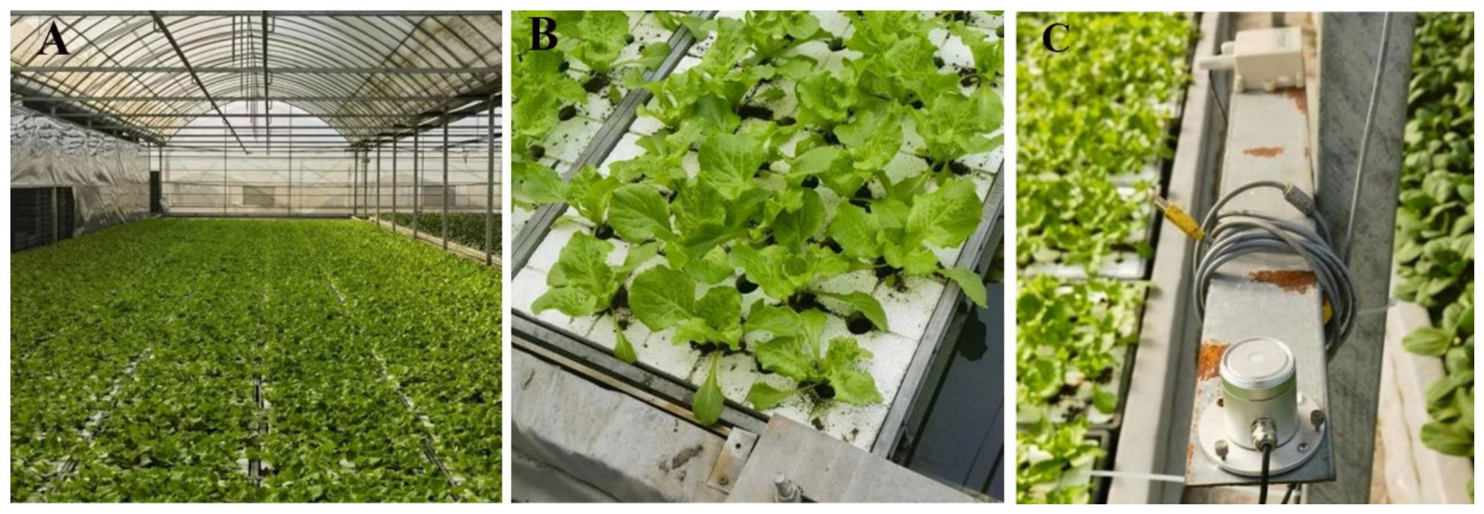
Figure 1. Lettuce cultivation experiment scene: (A) Lettuce cultivation environment in a greenhouse, using a 10 m × 8.6 m glass greenhouse. (B) Lettuce floating soilless cultivation. (C) Environmental data collection, including sensors for temperature, humidity, carbon dioxide concentration, and photosynthetically active radiation (PAR).
Horticulturae 12 01063 g001
Figure 2. Dataset Slices (A) Camera fixed position, shooting vertically downward towards the ground. (B) Fixed view of the field image acquisition, containing two complete cultivation trays. (C) Preset sampling method for the physiological data of lettuce; five seedlings at fixed positions were sampled from each plug tray. Dataset images were cropped from scene photos. Red triangles mark the five sampled plants from each tray.
Horticulturae 12 01063 g002
Figure 3. Two Ways of SA embedding: (a) ResNet50_SA_R. (b) ResNet50_SA_E. Note: The left figure introduces the multi-head self-attention mechanism in the way of side connection, and the attention information affects the propagation of backbone features; the right image shows how the multi-head self-attention module is embedded in the ResNet50 backbone instead of a stage.
Horticulturae 12 01063 g003
Figure 4. Multi-head self-attention mechanism: We implemented the two SA combination ideas mentioned earlier and designed two series of model structures named ResNet50_SA_R and ResNet50_SA_E, which contain three variants, V1 to V3, respectively. In the ResNet50_SA_R series, SA is added as additional information from the output of Stage1 and the output of each Stage. The difference between the three variants lies in the Stage level to which the SA output is connected, and V1 to V3 regression at the output layer of Stages 2, 3, and 4, respectively.
Horticulturae 12 01063 g004
Figure 5. Two series model V1 version structures (A) Structure of ResNet50_SA_RV1; implementation of side connection embedding. (B) Structure of ResNet50_SA_EV1; implementation of encoder internal embedding.
Horticulturae 12 01063 g005
Figure 6. Partial feature map output before and after improvement: (AD) are the output feature map images of the image on layers 1 to 4 of ResNet50; (EH) are the output feature map images of layers 1 to 4 of the image in ResNet50_SA_RV1. The maps illustrate differences in intermediate activation patterns and spatial feature representation after architectural modification.
Horticulturae 12 01063 g006
Figure 7. The loss decreases during the training process: (a) comparing the loss reduction process of seven neural network models trained from 0 to 400 iterations, (b) truncating the loss reduction process from 200 to 1000 iterations. (c) The validation set loss reduction process for all 50 epochs of the seven neural network models, and (d) the loss reduction process for 40 to 50 epochs.
Horticulturae 12 01063 g007
Figure 8. Fitting results on the fixed test dataset: (ac) prediction results of the ResNet50_SA_R-series models (RV1, RV2, and RV3); (df) prediction results of the ResNet50_SA_E-series models (EV1, EV2, and EV3); and (g) prediction results of the vanilla ResNet50 baseline. Note: Blue dots represent the predicted vs. true nitrogen content values, the dashed black line denotes the ideal 1:1 reference line, and the solid red line indicates the linear fit of the prediction results.
Horticulturae 12 01063 g008
Table 1. Different Model Accuracies.
Model (Pretrained)DatasetAccuracyParameters (M)GFLOPS
R2RMSEMAE
ResNet50Validation0.7912.776.823.532.015
Test0.819.946.29
ResNet50_SA_EV1Validation0.7515.328.8861.5816.58
Test0.7214.418.44
ResNet50_SA_EV2Validation0.6311.857.65170.9116.34
Test0.6216.6910.11
ResNet50_SA_EV3Validation0.7411.978.48623.416.66
Test0.4411.627.15
ResNet50_SA_RV1Validation0.898.417.6662.817.065
Test0.927.093.97
ResNet50_SA_RV2Validation0.517.4210.46180.1117.245
Test0.6311.676.58
ResNet50_SA_RV3Validation0.8610.856.57663.5417.645
Test0.899.326.57
Table 2. Grouped five-fold cross-validation results of all evaluated architectures.
ModelR2RMSE (mg/g)MAE (mg/g)
ResNet50_SA_RV1 (proposed)0.92 ± 0.037.16 ± 1.774.06 ± 1.58
ResNet50 (baseline)0.81 ± 0.069.91 ± 1.966.31 ± 1.54
ResNet180.80 ± 0.0611.53 ± 2.197.73 ± 1.37
SqueezeNet1_10.75 ± 0.0412.85 ± 3.419.09 ± 1.93
ShuffleNetV20.62 ± 0.0416.04 ± 2.8811.57 ± 0.95
RegNet0.49 ± 0.1118.54 ± 4.7812.30 ± 2.14
Note: Values are mean ± SD across five grouped folds, macro-averaged across N, P, and K. Units: mg/g dry mass.
Disclaimer/Publisher’s Note: The statements, opinions and data contained in all publications are solely those of the individual author(s) and contributor(s) and not of MDPI and/or the editor(s). MDPI and/or the editor(s) disclaim responsibility for any injury to people or property resulting from any ideas, methods, instructions or products referred to in the content.