Integrating GWAS and Machine Learning to Dissect the Genetic Basis of Flowering Time and Vernalization-Type Differentiation in Brassica napus

Highlights

Main findings

• Two FarmCPU GWAS covariate models separately detected 32 and 27 suggestive flowering-time-associated SNPs in 894 rapeseed accessions with over 8.39 million high-quality SNPs.
• ExtraTreesRegressor machine learning identified 18,854 high-contribution SNPs, which were merged into 997 ML-derived candidate QTL intervals, hereafter referred to as ML-QTLs. Interval-level integration of ML-QTLs with GWAS-derived QTLs prioritized 34 GWAS- and ML-supported candidate regions associated with flowering time and vernalization-type differentiation.
• The 34 GWAS- and ML-supported candidate regions harbor putative flowering regulatory genes (FLC, FRI-like, VIN3-like, SOC1, ELF3, CO-like, AP1-like and gibberellin pathway genes). Multi-SNP genotype combinations within these regions were significantly associated with flowering-time variation and showed different distribution patterns among three ecotype groups (spring, semi-winter, winter rapeseed).

Implications

• The integrated GWAS-machine learning framework offers a complementary strategy to dissect complex quantitative traits with strong population ecotype differentiation in allopolyploid crops.
• The prioritized candidate regions, putative flowering-related genes, and candidate SNP marker sets provide valuable genomic resources for future marker development, functional validation, flowering-time improvement, and regional adaptation studies in rapeseed.

Abstract

Flowering time is an important trait affecting regional adaptation and yield stability in rapeseed (Brassica napus). To dissect the genetic basis of flowering time and vernalization-type differentiation in B. napus, this study integrated genome-wide SNPs, flowering-time phenotypes, vernalization types, and geographic origin information to establish a candidate QTL discovery framework combining genome-wide association study (GWAS) and machine learning. Based on 8,387,529 high-quality SNPs, GWAS was performed using the FarmCPU model under two covariate settings: a PC-corrected model and a PC + vernalization type-corrected model. These two models identified 32 and 27 suggestive SNPs, respectively. In parallel, ExtraTreesRegressor was used to estimate the feature contribution of SNPs to flowering-time prediction, leading to the identification of 18,854 ML_delta10SD high-contribution SNPs, which were further merged into 997 ML-derived candidate QTL intervals, hereafter referred to as ML-QTLs. By integrating GWAS-derived QTLs and ML-QTLs at the interval level, 34 GWAS- and ML-supported candidate regions were prioritized. Candidate gene annotation revealed that these regions contained genes related to flowering regulation, including FLC, FRIGIDA-like, VIN3-like, SOC1, ELF3, CONSTANS-like, APETALA1-like, and genes involved in the gibberellin pathway. Top-SNP genotypic effect analysis and multi-SNP genotype combination analysis further showed that genetic variation within representative candidate regions was significantly associated with flowering-time differences and vernalization-type differentiation. Predictive modeling indicated that candidate markers selected by GWAS and machine learning showed predictive potential within the present population. Overall, this study prioritized a set of GWAS- and ML-supported candidate regions and putative candidate genes associated with flowering time in B. napus from the complementary perspectives of statistical association and machine learning-based predictive contribution, providing candidate resources for future marker development, functional validation, and adaptive improvement in rapeseed.

1. Introduction

Rapeseed (Brassica napus L.) is one of the most important oilseed crops worldwide and serves as a major source of edible vegetable oil, plant protein feed, and industrial raw materials [1,2]. As an allotetraploid crop, B. napus originated from hybridization between B. rapa and B. oleracea, followed by chromosome doubling, and possesses a complex A and C subgenome structure with abundant genetic variation. Long-term domestication and breeding selection have generated diverse ecologically adapted types of B. napus, including spring, semi-winter, and winter types. These types differ substantially in vernalization requirement, cold tolerance, vegetative growth duration, and flowering time [3,4,5]. Therefore, elucidating the genetic basis of important agronomic traits in B. napus is essential for adaptive improvement and molecular breeding.

Flowering time is a key agronomic trait that affects regional adaptation, yield formation, and maturity arrangement in B. napus [6]. Appropriate flowering time enables plants to coordinate vegetative and reproductive growth and to avoid unfavorable environmental conditions such as low temperature, heat, or drought, thereby influencing seed set, yield stability, and cultivation adaptability [7]. Flowering time in B. napus is jointly regulated by genetic factors, environmental conditions, and their interactions, among which vernalization response is a major determinant of flowering differences among ecotypes [8,9]. Winter-type accessions generally require prolonged exposure to low temperatures to complete the transition from vegetative to reproductive growth, whereas spring-type accessions have a weak vernalization requirement, and semi-winter accessions are intermediate between the two. Therefore, genetic dissection of flowering time in B. napus should consider not only phenotypic variation itself but also the effects of vernalization-type differentiation and population structure on genetic signals.

At the molecular level, the flowering-time regulatory network in B. napus is partially conserved with that of the model plant Arabidopsis thaliana. However, because B. napus is an allopolyploid species, many flowering regulatory genes have multiple homologous copies in the A and C subgenomes, which may have undergone functional divergence or subfunctionalization. Previous studies have shown that FLC, FRIGIDA, VIN3, SOC1, FT, ELF3, CONSTANS, APETALA1, and genes related to gibberellin signaling are involved in the regulation of flowering time [10,11]. Among them, FLC is an important floral repressor in the vernalization pathway, while FRIGIDA can affect FLC expression, and vernalization promotes floral transition by repressing FLC activity [12,13]. In B. napus, allelic variation in FRIGIDA homologs has been shown to be associated with flowering-time variation and differentiation among growth types. Therefore, genome-wide identification of candidate loci and genes related to these pathways is important for understanding the genetic basis of flowering time and vernalization ecotype differentiation in B. napus.

With the development of high-throughput sequencing and large-scale SNP genotyping technologies, genome-wide association study (GWAS) has become an important approach for dissecting the genetic basis of complex quantitative traits in crops [14,15]. By exploiting historical recombination in natural populations, GWAS enables the detection of trait-associated loci at relatively high resolution. In recent years, GWAS has been widely applied to important agronomic traits in B. napus, including yield, oil content, quality, stress resistance, and flowering time, leading to the identification of numerous candidate loci and genes [16,17]. For flowering time in B. napus, previous GWAS studies using natural populations and multi-environment phenotypic data have revealed the complex genetic architecture of this trait and identified candidate genes related to photoperiod response, vernalization, and flowering regulation [6,18]. These studies demonstrate that GWAS is an effective strategy for candidate gene discovery in complex traits of B. napus. However, conventional GWAS is usually based on single-marker statistical tests and mainly captures linear associations between individual SNPs and phenotypes. For complex traits such as flowering time, which are influenced by multiple genes, small-effect loci, population structure, vernalization type, and potential nonlinear effects, GWAS alone may not fully capture all trait-related genetic signals. In addition, under strong population structure or ecotype differentiation, some association signals may reflect both phenotypic differences and population differentiation, requiring careful interpretation using different covariate models. FarmCPU iteratively uses fixed-effect and random-effect models to control false positives while reducing the risk of false negatives and has been widely used for GWAS of complex traits. Therefore, in the genetic analysis of flowering time in B. napus, constructing both a PC-corrected model and a PC + vernalization type-corrected model can help distinguish overall flowering-time-associated signals from genetic effects that remain detectable after accounting for vernalization type. In recent years, machine learning methods have been increasingly applied to crop complex trait prediction and candidate marker selection because of their ability to handle high-dimensional genotype data, capture complex relationships among variables, and provide feature importance estimates [19]. Unlike GWAS-derived p-values, feature importance values from machine learning models can evaluate the relative contribution of SNPs to phenotypic prediction. Therefore, machine learning should not be considered a replacement for GWAS-based statistical significance testing, but rather a complementary approach that can identify potentially important markers from the perspective of predictive contribution. Previous crop studies have shown that machine learning-based feature selection and interpretable models can be used to screen key SNPs and assist in genetic dissection and genomic prediction of complex traits [20,21]. For flowering time in B. napus, integrating GWAS-based statistical association signals with machine learning-based predictive contribution signals may help prioritize candidate regions from complementary perspectives.

Based on this rationale, the present study focused on flowering time in B. napus and integrated genome-wide SNPs, flowering-time phenotypes, vernalization type, and geographic origin information to establish a genetic dissection framework combining GWAS and machine learning. Using publicly available phenotypic and resequencing data, this study performed an integrative reanalysis to prioritize candidate regions associated with flowering time and vernalization-type differentiation. First, FarmCPU was used to perform GWAS under both the PC-corrected model and the PC + vernalization-type-corrected model to identify flowering-time-associated loci. Next, ExtraTreesRegressor was used to estimate the feature contribution of genome-wide SNPs to flowering-time prediction, and ML_delta10SD high-contribution SNPs were selected. GWAS-associated SNPs and machine learning-derived high-contribution SNPs were further merged into GWAS-derived QTLs and ML-derived candidate QTL intervals, hereafter referred to as ML-QTLs, respectively. Interval overlap between the two types of QTLs was then used to identify GWAS- and ML-supported candidate regions. Candidate genes related to flowering regulation within these QTLs were annotated, and the relationships between candidate regions, flowering-time variation, and vernalization-type differentiation were further evaluated through top-SNP genotypic effect analysis, multi-SNP genotype combination analysis, and assessment of the predictive potential of candidate marker sets. This study aims to dissect the genetic basis of flowering time and vernalization-type differentiation in B. napus from the complementary perspectives of statistical association and machine learning-based predictive contribution, thereby providing candidate genomic regions, putative candidate genes, and marker resources for future functional validation, marker development, and adaptive improvement in rapeseed.

2. Materials and Methods

2.1. Plant Materials and Phenotypic Data

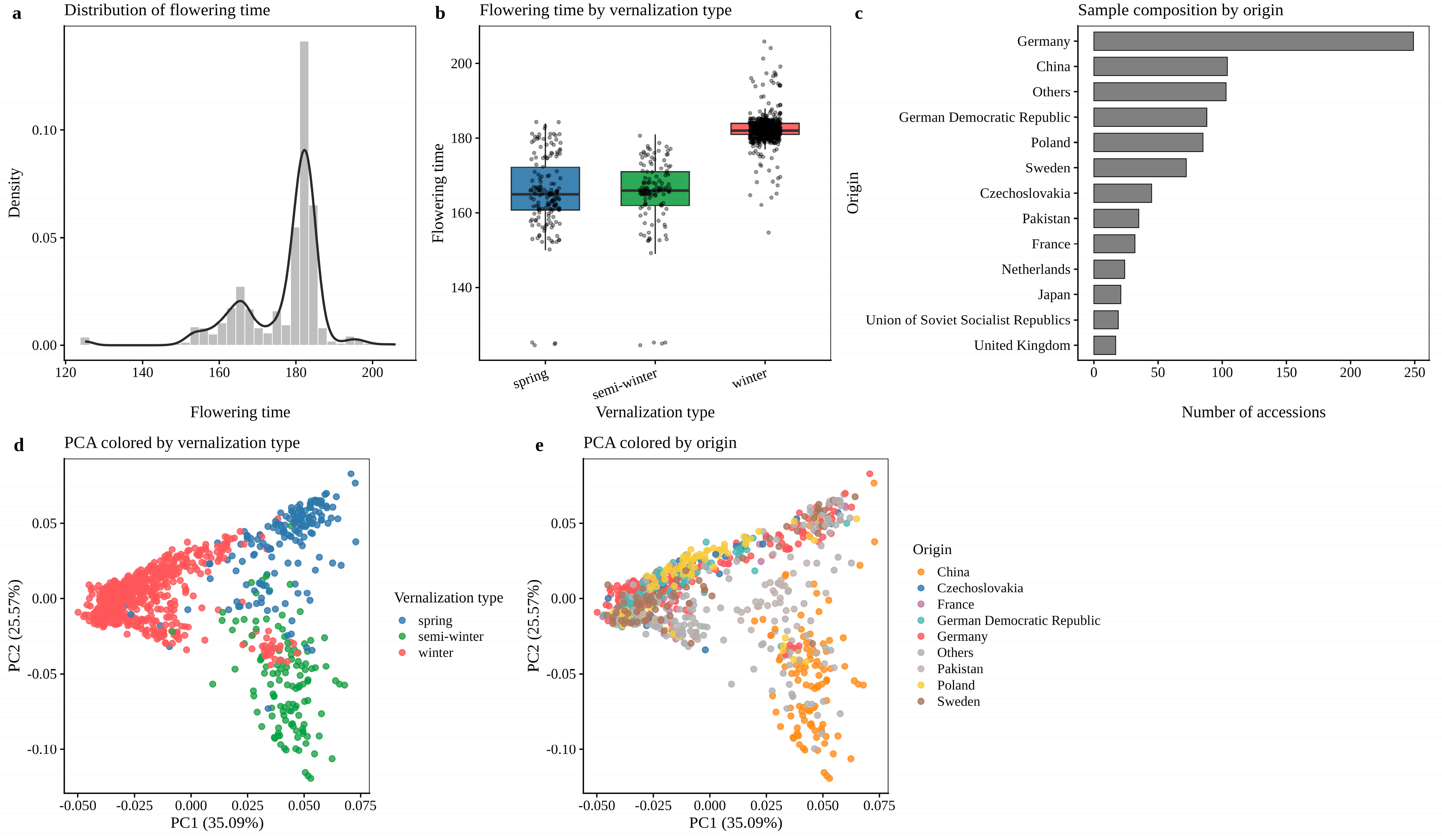
A natural population of B. napus was used in this study to investigate the genetic basis of flowering time. Flowering-time phenotypes, vernalization types, and geographic origin information were collected for each accession. The vernalization types were classified into three categories: spring, semi-winter, and winter types. These data were obtained from the study of Wu et al. (2018) [22]. Thus, the present study represents an integrative reanalysis of publicly available phenotypic and genomic resources rather than the generation of a new experimental population. To ensure consistency in downstream analyses, only accessions with both flowering-time records and genotypic data were retained. In total, 894 accessions were included in the final analysis. Descriptive statistics were then performed for flowering time to characterize its distribution across the whole population. In addition, flowering-time differences among accessions with different vernalization types were compared. This analysis was conducted to evaluate whether variation in flowering time was associated with differentiation among vernalization ecotypes, thereby providing a phenotypic basis for subsequent genome-wide association study and machine learning analyses.

2.2. Sequencing Data and SNP Calling

The whole-genome resequencing data used in this study were obtained from the NCBI database under the accession number SRP155312 (https://www.ncbi.nlm.nih.gov/sra/SRP155312) (accessed on 6 May 2026). Raw paired-end sequencing reads for each accession were downloaded according to the sample correspondence information. Quality control of the raw reads was performed using fastp to remove adapter sequences, low-quality bases, and low-quality reads. The resulting clean reads were used for subsequent read alignment. The clean reads were aligned to the chromosome-level Brassica napus reference genome Da-Ae (RefSeq assembly accession: GCF_020379485.1) (https://www.ncbi.nlm.nih.gov/datasets/genome/GCF_020379485.1/) (accessed on 6 May 2026), which contains 19 chromosomes corresponding to the A and C subgenomes of B. napus. Read alignment was performed using BWA-MEM (v0.7.17) [23]. SAMtools (v1.23.1) was then used to convert, sort, and index the alignment files, generating sorted BAM files for each sample [24]. To ensure the reliability of variant detection, basic quality checks were performed on the BAM files, and poorly aligned reads were removed. The high-quality alignment results were retained for genome-wide variant calling. Multi-sample variant calling was conducted using bcftools (v1.23.1) [25]. Briefly, bcftools mpileup was first used to generate sequencing-depth and base-support information across genomic sites based on the BAM files of all samples, followed by variant calling using bcftools call to obtain the raw VCF file. To improve the reliability of the SNP dataset, stringent filtering was applied to the raw variants. Low-quality variants, variants with a high missing rate, sites with insufficient or abnormal sequencing depth, and variants with low minor allele frequency were removed. Subsequently, only biallelic SNPs were retained, whereas InDels, multiallelic variants, and variants located on non-standard chromosomes were excluded.

The final high-quality SNP dataset was used for population structure analysis, genome-wide association study, machine learning-based feature importance analysis, and genotype-effect analysis. The filtered SNP dataset was further converted into PLINK format, including binary genotype files, BIM/FAM files, and an additive dosage matrix according to the requirements of different downstream analyses [26]. After quality control and sample matching, a total of 8,387,529 high-quality SNPs were retained for the genetic analysis of flowering time.

2.3. Population Structure Analysis

To evaluate the potential influence of population structure on flowering-time variation, principal component analysis (PCA) was performed based on genome-wide SNPs [27]. Prior to PCA, linkage disequilibrium pruning was conducted to reduce the effect of highly correlated markers. The pruned SNP dataset was then used to calculate principal component scores for each accession. A PCA scatter plot was generated using the first two principal components, with accessions colored according to vernalization type and geographic origin, respectively. This visualization was used to examine the genetic relationships among accessions and the overall pattern of population differentiation. Based on the PCA results, the top principal components were selected as covariates in subsequent genome-wide association analyses to correct for population structure.

2.4. Genome-Wide Association Analysis

Genome-wide association analysis of flowering time was performed using the FarmCPU model [28]. To evaluate the influence of vernalization type on flowering-time association signals, two covariate models were constructed. In the first model, principal components were included as covariates in FarmCPU to correct for the effect of population structure. This model was referred to as the FarmCPU-PC model. In the second model, vernalization type was further incorporated as an additional covariate together with the principal components. This model was designed to identify genetic loci that remained associated with flowering time after accounting for differentiation among vernalization ecotypes and was referred to as the FarmCPU-PC-Type model.

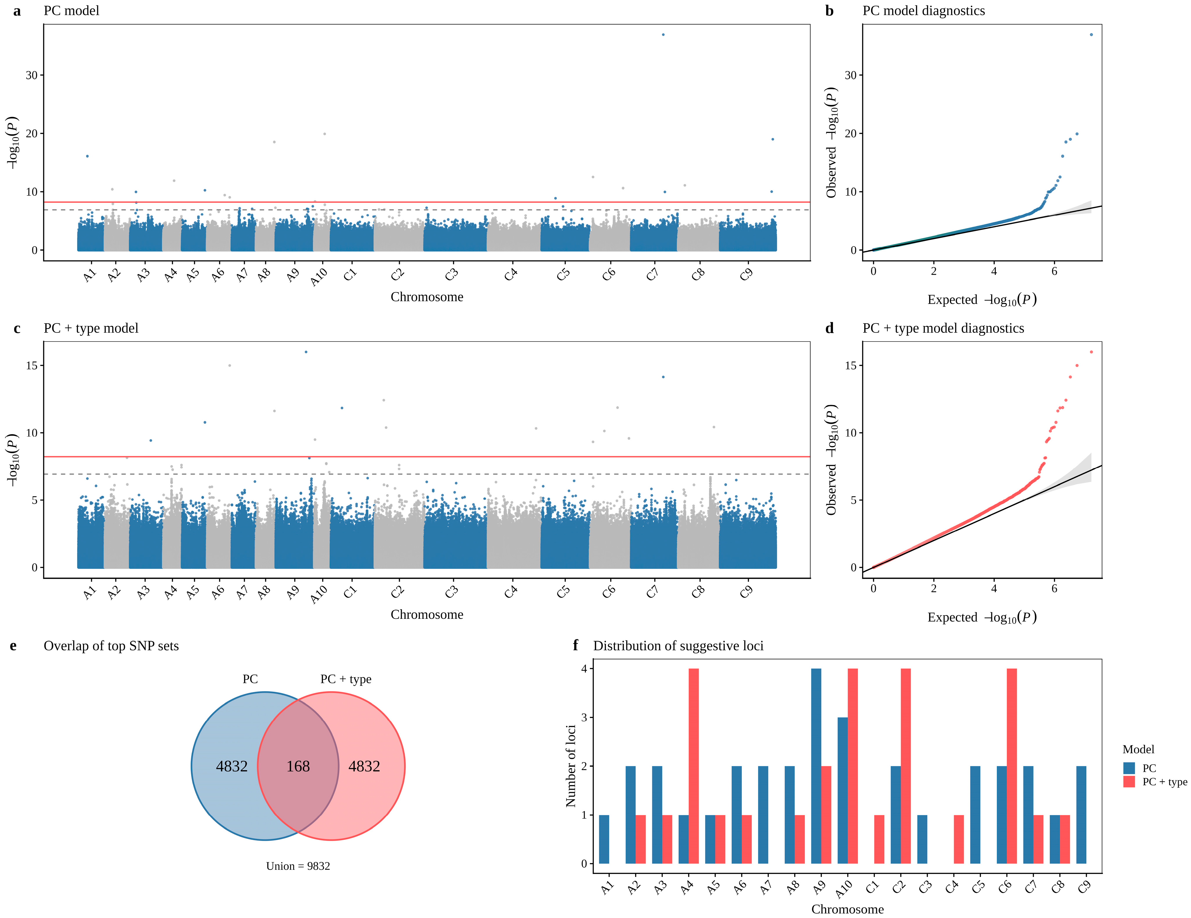
For each SNP, the FarmCPU model estimated the statistical significance of its association with flowering time. The Bonferroni-corrected significance threshold was defined as 0.05 divided by the total number of SNPs tested across the genome, whereas the suggestive threshold was defined as 1 divided by the total number of SNPs tested. In this study, approximately 8,387,529 SNPs were used for genome-wide testing; therefore, the Bonferroni-corrected significance threshold was 5.96 × 10⁻⁹, and the suggestive threshold was 1.19 × 10⁻⁷. SNPs reaching the suggestive threshold were used for the subsequent construction of GWAS-derived QTLs.

2.5. Machine Learning-Based Analysis of SNP Feature Contribution

To complement the GWAS results from a predictive perspective, machine learning models were further constructed to evaluate the contribution of genome-wide SNPs to flowering-time variation. In this analysis, flowering time was used as the response variable, and the SNP additive dosage matrix was used as the explanatory variable. Because of the large number of genome-wide SNPs, it was computationally infeasible to include all markers in a single model. Therefore, a block-wise ExtraTreesRegressor strategy was adopted. Specifically, genome-wide SNPs were first ordered by chromosome and physical position and then divided into multiple consecutive SNP blocks with a fixed block size of 50,000 SNPs [29,30]. For each block, an ExtraTreesRegressor model was trained independently. The model parameters were set as follows: n_estimators = 200, max_features = “sqrt”, min_samples_leaf = 2, and random_state = 2026 + chunk index to ensure reproducibility. After model training, the feature importance value of each SNP was extracted and used as its machine learning-based feature contribution score. The SNP importance results from all blocks were then merged to obtain the genome-wide distribution of ML_importance values. Because feature importance values were estimated independently within each SNP block, importance values across blocks may not be strictly comparable to global importance values estimated from a single whole-genome model. Therefore, this analysis was interpreted as block-wise ML-based SNP contribution screening rather than a formal statistical significance test. Accordingly, SNPs identified by the machine learning analysis were referred to as ML high-contribution SNPs rather than ML significant SNPs.

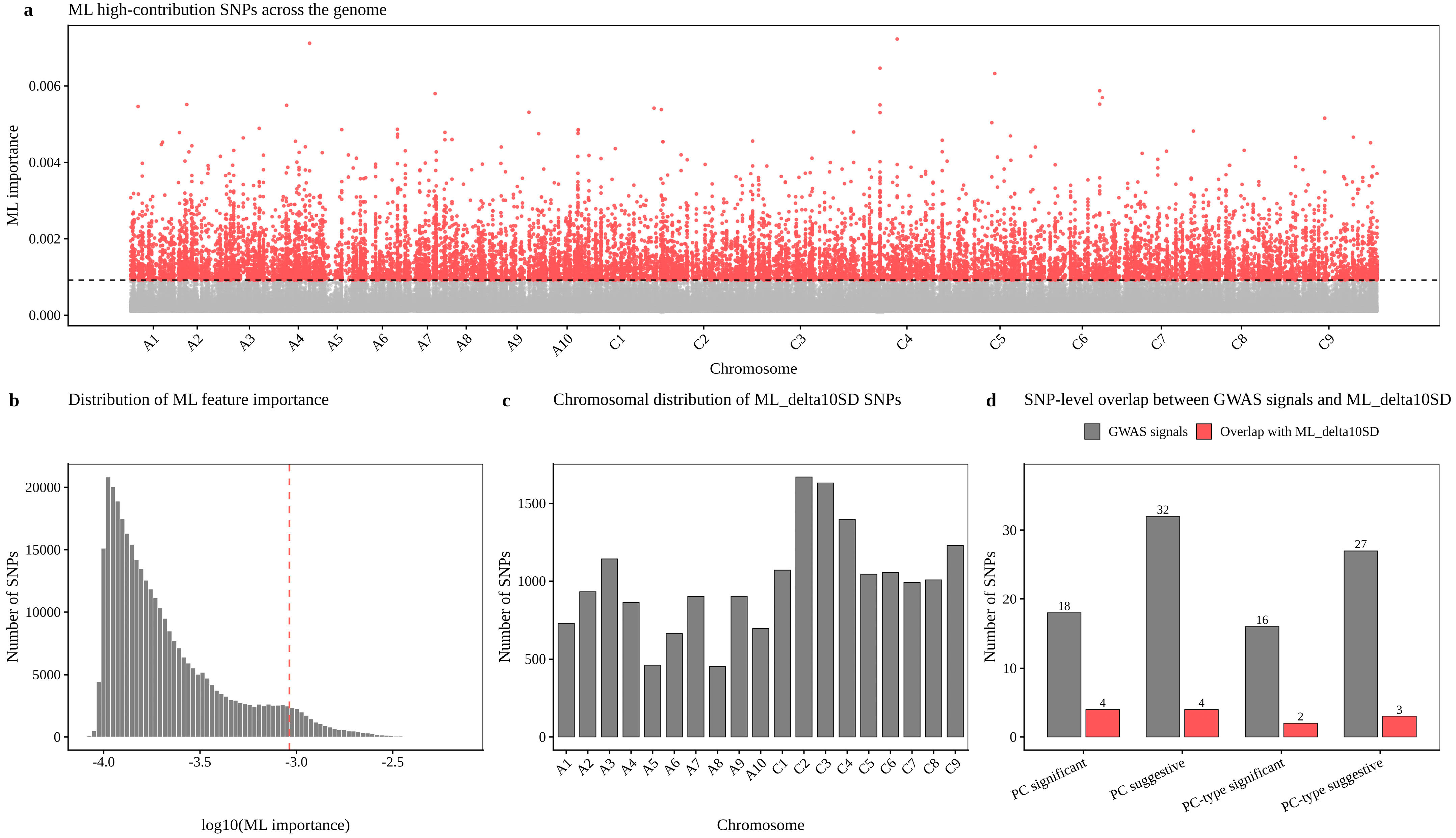
Following the rationale of previous ML-QTL studies that identify candidate markers based on the degree of deviation in feature contribution, the mean and standard deviation of genome-wide SNP importance values were calculated. SNPs with importance values greater than the mean plus 10 standard deviations were defined as ML_delta10SD high-contribution SNPs: ML_importance > mean(ML_importance) + 10 × SD(ML_importance). These ML_delta10SD high-contribution SNPs were subsequently used to construct ML-derived ML-QTLs.

2.6. Identification of GWAS-Derived QTLs and ML-Derived ML-QTLs

Both GWAS and machine learning analyses initially identify individual SNPs. However, a single SNP usually serves as a representative marker of an underlying genetic-effect region and is not necessarily the causal variant itself. Considering the presence of linkage disequilibrium among neighboring SNPs, multiple associated SNPs or high-contribution SNPs located within the same genomic region may collectively indicate the same genetic-effect locus. Therefore, candidate SNPs were further merged into QTL intervals based on their physical positions, allowing the analysis to be extended from the single-SNP level to the genomic-interval level.

For GWAS-derived QTLs, SNPs reaching the suggestive threshold were extracted separately from the FarmCPU-PC and FarmCPU-PC-Type models. These candidate SNPs were mapped according to their chromosome and physical position. Each candidate SNP was extended by 250 kb upstream and downstream, and overlapping windows on the same chromosome were merged into a single GWAS-derived QTL interval. For ML-derived ML-QTLs, ML_delta10SD high-contribution SNPs were first mapped to chromosomes and physical positions based on the PLINK BIM file. The same physical window merging strategy used for GWAS-derived QTLs was then applied to combine adjacent or overlapping high-contribution SNP intervals into ML-derived ML-QTLs. The resulting ML-QTLs represent machine learning-derived candidate genomic intervals formed by clusters of ML high-contribution SNPs, rather than classical QTLs identified through linkage mapping.

2.7. Genotypic Effect Analysis of Candidate QTLs

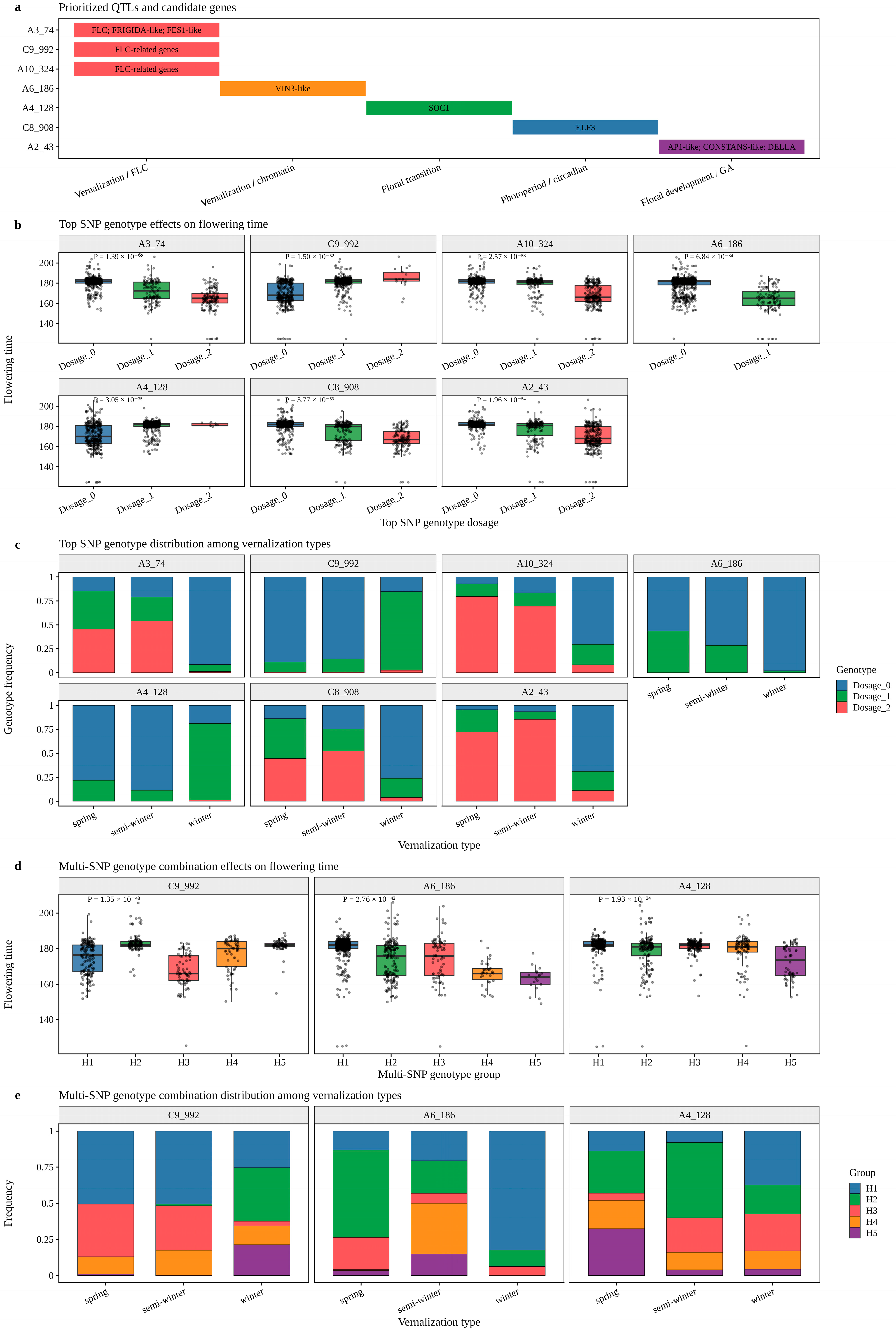
To further evaluate the relationship between representative GWAS- and ML-supported candidate regions and flowering-time variation, representative QTLs containing typical flowering-related candidate genes were selected for genotypic effect analysis. For each candidate QTL, the most representative top SNP within the interval was selected for analysis based on the highest overall priority. The genotype of each top SNP was encoded as an allelic dosage of 0, 1, or 2. Flowering-time differences among the different dosage genotypes were then compared, and nonparametric tests were used to evaluate the statistical significance of these differences. In addition, the frequency distribution of different dosage genotypes of the top SNP was calculated across accessions with different vernalization types. This analysis was performed to examine the relationship between candidate loci and differentiation among vernalization ecotypes.

Furthermore, multi-SNP genotype combination analysis was conducted for selected representative candidate gene regions. For each candidate region, genotype combinations of multiple SNPs within the interval were extracted, and major combination types with sufficient sample sizes were retained. Within each region, the different combinations were labeled as H1, H2, H3, H4, and H5. Flowering-time differences among these multi-SNP genotype combinations were then compared, and their distribution patterns among spring, semi-winter, and winter accessions were analyzed. It should be noted that the labels H1, H2, and so on only represent the major genotype combinations within a specific QTL region. Therefore, the same label in different regions does not indicate the same genotype combination.

2.8. Evaluation of the Predictive Potential of Different Marker Sets

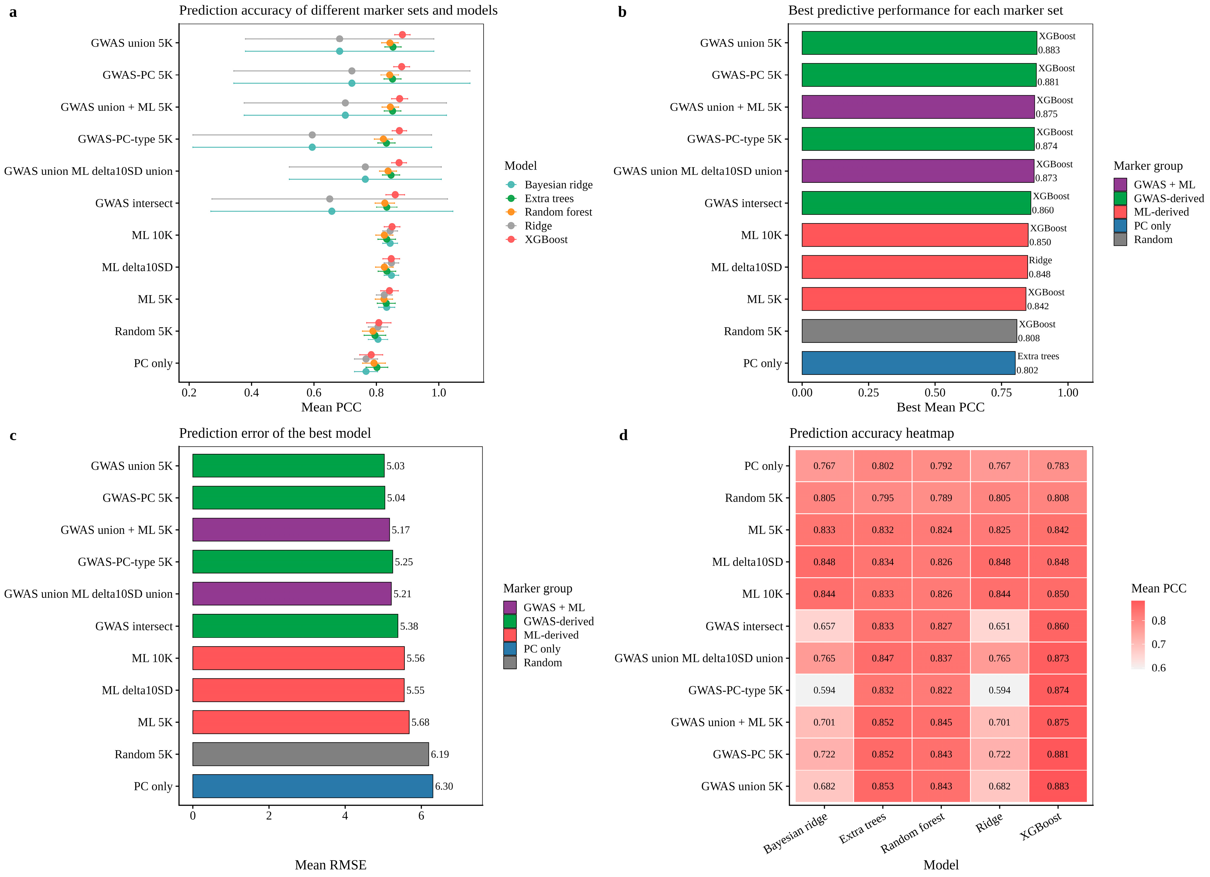
To evaluate the predictive potential of GWAS- and machine learning-selected markers for flowering-time prediction within the present population, different marker sets were constructed and subjected to predictive modeling. These marker sets included a PC-only baseline, random SNP sets, GWAS-derived SNP sets, ML-derived SNP sets, and combined GWAS + ML SNP sets. All SNPs were encoded as additive dosages of 0, 1, and 2 and were matched with the flowering-time phenotypic data.

Multiple prediction models were compared, including Ridge regression, Bayesian Ridge regression, ExtraTrees, Random Forest, and XGBoost. Model performance was evaluated using repeated five-fold cross-validation [31,32,33,34]. The evaluation metrics included Pearson’s correlation coefficient, coefficient of determination (R²), root mean square error, and mean absolute error. Because flowering time was strongly associated with population structure and vernalization-type differentiation, prediction results were interpreted as marker-set predictive potential in the current population rather than as direct evidence of broad breeding utility in independent populations.

To facilitate reader understanding and ensure consistent use of terminology throughout the manuscript, abbreviations related to GWAS models, ML-derived marker sets, candidate intervals, and prediction baselines are summarized in

Table 1. Summary of abbreviations and marker-selection strategies used in this study.

Abbreviation	Full Name/Meaning	Description
FarmCPU-PC	FarmCPU model corrected by principal components	GWAS model using PCs as covariates
FarmCPU-PC-Type	FarmCPU model corrected by principal components and vernalization type	GWAS model using PCs and vernalization type as covariates
GWAS-PC	SNPs or QTLs derived from the FarmCPU-PC model	Association signals detected without vernalization-type correction
GWAS-PC-Type	SNPs or QTLs derived from the FarmCPU-PC-Type model	Association signals detected after vernalization-type correction
ML_delta10SD	ML importance > mean + 10SD	Empirical threshold for ML high-contribution SNPs
ML high-contribution SNPs	SNPs prioritized by ML feature importance	SNPs selected from ExtraTreesRegressor feature contribution scores
ML-QTL	Machine learning-derived candidate QTL interval	Candidate interval formed by merging ML high-contribution SNPs
GWAS-derived QTL	QTL interval derived from GWAS-suggestive SNPs	SNPs were extended and merged according to physical position
GWAS- and ML-supported candidate region	Candidate region supported by both GWAS-derived QTLs and ML-QTLs	Prioritized candidate region used for downstream gene annotation
PC-only	Principal-component-only baseline	Prediction model using population structure only
Random 5K	Randomly selected 5000 SNPs	Random marker-set baseline for prediction

.

3. Results

3.1. Phenotypic Variation in Flowering Time and Population Structure Analysis

To characterize phenotypic variation in flowering time within the Brassica napus population, flowering-time phenotypes, vernalization types, and geographic origins were first summarized. Flowering time showed a continuous distribution across the population, indicating that this trait exhibits typical quantitative variation (Figure 1a). Clear differences in flowering-time distribution were observed among accessions with different vernalization types. Spring, semi-winter, and winter accessions displayed distinct flowering-time ranges and distribution patterns, suggesting that vernalization type is closely associated with flowering-time variation (Figure 1b). Analysis of geographic origin showed that the population consisted of accessions from diverse regions, with a relatively high proportion originating from China, as well as accessions from Europe and other regions (Figure 1c).

Principal component analysis based on genome-wide SNPs further revealed the population structure of the panel. When accessions were colored by vernalization type, spring, semi-winter, and winter accessions showed a certain degree of differentiation in the principal component space, indicating genetic background differences among vernalization types (Figure 1d). When accessions were colored by geographic origin, some accessions also exhibited origin-related clustering patterns, suggesting that geographic origin contributed to population structure to some extent (Figure 1e). Taken together, these results indicate that flowering-time variation in B. napus is closely associated with vernalization type and population structure. Therefore, both population structure and vernalization type should be considered in subsequent association analyses.

3.2. Identification of Flowering-Time-Associated Loci by FarmCPU-GWAS

To identify genetic loci associated with flowering time in Brassica napus, genome-wide association analysis was performed using the FarmCPU model. Considering the substantial influence of vernalization type on flowering time, two models were constructed: the FarmCPU-PC model and the FarmCPU-PC-Type model. In the FarmCPU-PC model, principal components were included as covariates to correct for population structure. In the FarmCPU-PC-Type model, vernalization type was further included as an additional covariate to detect loci that remained associated with flowering time after accounting for vernalization type.

In the FarmCPU-PC model, 32 SNPs reached the suggestive threshold, including 18 SNPs that exceeded the Bonferroni-corrected significance threshold (Figure 2a). The corresponding QQ plot showed that most observed p-values were largely consistent with the expected distribution, with clear deviation only in the tail. This pattern suggests that the model effectively controlled the overall false-positive rate while detecting strong association signals (Figure 2b). In the FarmCPU-PC-Type model, 27 SNPs reached the suggestive threshold, including 16 Bonferroni-significant SNPs (Figure 2c). The QQ plot also showed a clear tail deviation, indicating that genetic signals associated with flowering time remained detectable after correction for vernalization type (Figure 2d).

A further comparison of the top-ranked SNPs from the two models revealed limited overlap between their top 5000 SNP sets. Only 168 SNPs were shared between the FarmCPU-PC and FarmCPU-PC-Type models, whereas 4832 SNPs were specific to each model, resulting in a union of 9832 SNPs (Figure 2e). This result indicates that inclusion of vernalization type as a covariate substantially affected the ranking and selection of GWAS signals for flowering time. The distribution of suggestive loci across chromosomes also differed between the two models, suggesting that flowering-time-associated signals are distributed across multiple genomic regions (Figure 2f).

3.3. Identification of ML High-Contribution SNPs for Flowering Time Using Machine Learning

To complement the GWAS results from a predictive perspective, a block-wise ExtraTreesRegressor strategy was further applied to evaluate the feature contribution of genome-wide SNPs. By calculating the feature importance of each SNP, the relative contribution of individual SNPs to flowering-time prediction was estimated as ML-based contribution scores rather than statistical significance values. The genome-wide distribution of ML importance values showed that most SNPs had low contribution scores, whereas only a small proportion of SNPs exhibited relatively high contributions (Figure 3a,b). Based on the mean and standard deviation of genome-wide feature importance values, SNPs with ML_importance greater than the mean plus 10 standard deviations were selected as high-contribution SNPs. Using this criterion, a total of 18,854 ML_delta10SD high-contribution SNPs were identified. These high-contribution SNPs were distributed across multiple chromosomes, suggesting that flowering time in Brassica napus may be jointly regulated by multiple genomic regions (Figure 3c).

Further comparison between GWAS signals and ML_delta10SD SNPs revealed limited overlap at the single-SNP level between GWAS significant/suggestive SNPs and ML-derived high-contribution SNPs (Figure 3d). This result indicates that GWAS and machine learning did not capture completely identical signals. Instead, they may reflect flowering-time-related genetic variation from two complementary perspectives: statistical association and predictive contribution.

To evaluate whether the ML_delta10SD threshold affected the main results, a threshold sensitivity analysis was further performed using alternative cutoffs, including mean + 5SD, mean + 8SD, mean + 10SD, and mean + 12SD. As the threshold became more stringent, the number of ML high-contribution SNPs decreased, whereas the major GWAS-overlapping ML-QTLs and representative flowering-related candidate regions were largely retained. These results indicate that the main candidate regions were not solely dependent on the ML_delta10SD cutoff (Supplementary Table S2).

3.4. Interval-Level Integration of GWAS-Derived QTLs and ML-Derived ML-QTLs

Because GWAS and machine learning may identify different representative SNPs within the same genetic region, comparison based solely on SNP-level overlap may underestimate the concordance between the two approaches. Therefore, candidate SNPs were further merged into QTL intervals according to their physical positions, and GWAS and machine learning results were integrated at the QTL-interval level. The 32 suggestive SNPs identified by the FarmCPU-PC model were merged into 30 GWAS-derived QTLs, whereas the 27 suggestive SNPs identified by the FarmCPU-PC-Type model were merged into 24 GWAS-derived QTLs. In parallel, the 18,854 ML_delta10SD high-contribution SNPs were merged into 997 ML-derived candidate QTL intervals, hereafter referred to as ML-QTLs. The number of different types of QTLs are summarized in Figure 4a. By comparing the interval overlap between GWAS-derived QTLs and ML-derived ML-QTLs, 34 GWAS- and ML-supported candidate regions were prioritized for subsequent analyses.

These 34 high-confidence candidate QTLs were distributed across multiple chromosomes of the A and C subgenomes, indicating that flowering time in Brassica napus is influenced by multiple genomic regions (Figure 4b). According to their sources of support, six QTLs were jointly supported by the FarmCPU-PC model, the FarmCPU-PC-Type model, and machine learning; 16 QTLs were supported by both the FarmCPU-PC model and machine learning; and 12 QTLs were supported by both the FarmCPU-PC-Type model and machine learning (Figure 4c). These results suggest that integrating GWAS-based statistical association signals and machine learning-based predictive contribution signals at the QTL-interval level can effectively prioritize high-confidence candidate regions for flowering time.

3.5. Candidate Gene Annotation Within GWAS- and ML-Supported Candidate Regions

To further prioritize putative candidate genes within the GWAS- and ML-supported candidate regions, these candidate intervals were compared with the Brassica napus reference genome annotation. Genes located within each candidate interval were extracted, and flowering-related candidate genes were further prioritized based on functional annotations. The results show that different high-confidence QTL intervals contained varying numbers of annotated genes, and several QTLs harbored genes with clear flowering-related functional annotations (Figure 4d).

Based on functional annotations and keyword-based screening, multiple GWAS- and ML-supported candidate regions were found to contain genes potentially involved in flowering regulation. These genes were associated with several functional categories, including vernalization regulation, floral repression, photoperiod response, circadian rhythm, flowering pathway integration, floral meristem formation, and gibberellin signaling (Figure 4e). Representative candidate regions contained genes annotated as FLC, FRIGIDA-like, VIN3-like, SOC1, ELF3, CONSTANS-like, APETALA1-like, and gibberellin pathway-related genes. These results suggest that the GWAS- and ML-supported candidate regions identified through the integration of GWAS and machine learning contain biologically plausible putative candidate genes related to flowering-time regulation.

Detailed annotations of the 34 GWAS- and ML-supported candidate regions, flowering-related putative candidate genes, and all annotated genes located within these regions are provided in Supplementary Table S3.

3.6. Genotypic Effects of Representative GWAS- and ML-Supported Candidate Regions on Flowering Time

To further evaluate the relationship between high-confidence candidate QTLs and flowering-time variation, seven representative QTLs containing flowering-related candidate genes were selected for genotypic effect analysis. These QTLs included A3_74, C9_992, A10_324, A6_186, A4_128, C8_908, and A2_43. The candidate genes within these regions were associated with multiple flowering-related pathways, including FLC/FRIGIDA-like regulation, VIN3-like vernalization response, SOC1-mediated floral transition, ELF3-related circadian regulation, APETALA1-like floral meristem identity, CONSTANS-like photoperiod response, and gibberellin-related pathways (Figure 5a;

Table 2. Representative GWAS- and ML-supported candidate regions selected for genotypic effect analysis.

QTL	Candidate Gene	Pathway	No. of Accessions	No. of Genotype Combinations	Kruskal–Wallis p
A10_324	FLC-related genes	Vernalization/FLC	658	18	6.35 × 10−56
A2_43	AP1-like; CONSTANS-like; DELLA	Floral development/GA	730	20	3.65 × 10−53
C9_992	FLC-related genes	Vernalization/FLC	823	22	1.35 × 10−48
A3_74	FLC; FRIGIDA-like; FES1-like	Vernalization/FLC	777	16	7.46 × 10−48
A6_186	VIN3-like	Vernalization/chromatin	861	9	2.76 × 10−42
C8_908	ELF3	Photoperiod/circadian	768	24	1.12 × 10−41
A4_128	SOC1	Floral transition	806	11	1.93 × 10−34

).

For each representative QTL, one top SNP was selected, and its genotype was classified into Dosage_0, Dosage_1, and Dosage_2 according to allelic dosage. Most representative QTLs showed clear differences in flowering time among top-SNP dosage classes, suggesting that these loci, or the genomic intervals in which they are located, are closely associated with flowering-time variation (Figure 5b). Further analysis of the frequency distribution of top-SNP dosage classes among spring, semi-winter, and winter accessions showed that some dosage classes were unevenly distributed among vernalization types (Figure 5c). These results indicate that the representative candidate QTLs may be associated not only with flowering-time variation but also with vernalization-type differentiation.

In addition to single top-SNP analysis, multi-SNP genotype combination analysis was performed for representative candidate-gene regions. For each QTL region, multi-SNP genotype combinations with sufficient sample sizes were retained for statistical analysis. Across the seven representative QTLs, the number of accessions included in the analysis ranged from 658 to 861, and the number of multi-SNP genotype combinations ranged from 9 to 24 (Table 1). Kruskal–Wallis tests showed highly significant flowering-time differences among multi-SNP genotype combinations in all seven QTL regions, with p-values ranging from 1.93 × 10⁻³⁴ to 6.35 × 10⁻⁵⁶ (Table 1). These results indicate that combined variation across multiple SNPs within candidate regions could effectively distinguish flowering-time phenotypes.

For visualization, three representative candidate-gene regions were further selected, and the major multi-SNP genotype combinations were labeled as H1, H2, H3, H4, and H5 within each region. It should be noted that these labels represent the major genotype combinations within each specific QTL region; therefore, the same label in different QTL regions does not indicate the same genotype combination. Clear flowering-time differences were observed among these multi-SNP genotype groups (Figure 5d). In addition, the distribution of genotype combinations differed among spring, semi-winter, and winter accessions (Figure 5e). Taken together, both the top-SNP dosage analysis and the multi-SNP genotype combination analysis support the association between genetic variation within high-confidence candidate QTLs and flowering-time variation, as well as their potential contribution to vernalization-type differentiation.

3.7. Predictive Potential of Different Candidate Marker Sets for Flowering Time

To evaluate the potential application value of GWAS- and machine learning-selected markers in flowering-time prediction, different marker sets were constructed and compared across multiple prediction models. These marker sets included PC-only, Random 5K, GWAS-derived SNP sets, ML-derived SNP sets, and combined GWAS + ML SNP sets. The prediction models included Bayesian Ridge, ExtraTrees, Random Forest, Ridge, and XGBoost.

The predictive performance of different marker sets and models is shown in Figure 6a. Overall, GWAS-derived marker sets showed relatively high predictive ability. Among them, the best-performing model for GWAS union 5K was XGBoost, with a mean Pearson correlation coefficient (PCC) of 0.883 and an RMSE of 5.03. Similarly, the best-performing model for GWAS-PC 5K was XGBoost, with a mean PCC of 0.881 and an RMSE of 5.04. For GWAS union + ML 5K, the best-performing model was also XGBoost, with a mean PCC of 0.875 and an RMSE of 5.17. For GWAS-PC-Type 5K, XGBoost achieved the best performance, with a mean PCC of 0.874 and an RMSE of 5.25. For GWAS union + ML_delta10SD union, the best-performing model was XGBoost, with a mean PCC of 0.873 and an RMSE of 5.21 (Figure 6b,c).

ML-derived marker sets also showed good predictive performance. The best-performing model for ML 10K was XGBoost, with a mean PCC of 0.850 and an RMSE of 5.56. For ML_delta10SD, Ridge achieved the best performance, with a mean PCC of 0.848 and an RMSE of 5.55. For ML 5K, the best-performing model was XGBoost, with a mean PCC of 0.842 and an RMSE of 5.68 (Figure 6b,c). The prediction-accuracy heatmap further showed that XGBoost, ExtraTrees, and Random Forest performed well across multiple marker sets, and that GWAS-derived and GWAS + ML marker sets generally exhibited higher predictive accuracy (Figure 6d).

Notably, the Random 5K and PC-only marker sets also showed relatively high predictive ability, with best mean PCC values of 0.808 and 0.802, respectively (Figure 6b). This result suggests that flowering-time prediction in Brassica napus is strongly influenced by population structure and differentiation among vernalization types. Therefore, these results mainly reflect the predictive potential of different candidate marker sets within the present population and should not be interpreted as evidence that candidate markers would necessarily outperform random markers in independent populations. Overall, the candidate markers identified by GWAS and machine learning contain abundant flowering-time-related genetic information and may have potential value for breeding applications.

4. Discussion

4.1. Flowering-Time Variation Is Closely Associated with Vernalization-Type Differentiation

Flowering time is an important agronomic trait that affects regional adaptation, maturity arrangement, and yield stability in B. napus [35]. In this study, flowering time showed continuous variation in the natural population, indicating that this trait has typical quantitative characteristics. Meanwhile, significant differences in flowering time were observed among spring, semi-winter, and winter accessions, suggesting that vernalization ecotype differentiation is an important factor contributing to flowering-time variation in B. napus. Previous studies have shown that different growth types of B. napus differ markedly in vernalization requirement, flowering time, and adaptation region, and that these differences are closely associated with genetic variation in genes involved in the vernalization pathway [6,13]. Consistently, the PCA results in the present study also revealed a certain degree of genetic differentiation among accessions with different vernalization types. Therefore, in the genetic dissection of flowering time in B. napus, correction for population structure alone may not be sufficient to fully distinguish flowering-time-associated signals from signals related to vernalization-type differentiation.

In this study, two GWAS models, FarmCPU-PC and FarmCPU-PC-Type, were used in parallel. The FarmCPU-PC model was designed to capture overall association signals related to flowering-time variation, whereas the FarmCPU-PC-Type model further accounted for vernalization type and was used to identify genetic effects that remained detectable after correction for vernalization-type differentiation. This dual-model strategy provides a more comprehensive framework for interpreting flowering-time association signals under the background of strong ecotype differentiation.

4.2. FarmCPU-GWAS Revealed Association Signals Related to Flowering Time

GWAS has been widely used to dissect the genetic basis of complex agronomic traits in B. napus, including flowering time, yield, oil content, and quality-related traits [36,37,38]. In the present study, the FarmCPU model was used to conduct GWAS for flowering time. By iteratively fitting fixed-effect and random-effect models, FarmCPU can improve the detection power for complex trait-associated loci while controlling the influence of population structure. The FarmCPU-PC model identified 32 suggestive SNPs, including 18 SNPs that reached the Bonferroni-corrected significance threshold. In comparison, the FarmCPU-PC-Type model detected 27 suggestive SNPs, including 16 Bonferroni-significant SNPs. Both models identified flowering-time-associated signals, but some association signals changed after vernalization type was included as an additional covariate. This result indicates that flowering-time-associated loci in B. napus include both genetic signals related to vernalization-type differentiation and loci that remain associated with flowering time after accounting for vernalization type [10].

These findings are consistent with the complex genetic architecture of flowering time in B. napus, which is shaped by both ecotype differentiation and environmental adaptation. Therefore, comparing GWAS results from models with and without vernalization-type correction provides a useful strategy for distinguishing broad flowering-time association signals from signals that remain detectable after vernalization-type correction.

4.3. Machine Learning Provides a Predictive Contribution Perspective Complementary to GWAS

Traditional GWAS is mainly based on single-SNP statistical testing and focuses on identifying loci that show significant linear associations with phenotypes. However, for complex traits, GWAS may have limited ability to capture nonlinear effects, multi-locus combination effects, and markers that contribute substantially to prediction but do not reach statistical significance in single-marker association tests. Machine learning methods can handle high-dimensional genotype data and evaluate the contribution of SNPs to phenotypic prediction through feature importance, making them a useful complement to GWAS.

In this study, a block-wise ExtraTreesRegressor strategy was used to perform feature contribution analysis for genome-wide SNPs, and 18,854 ML_delta10SD high-contribution SNPs were identified. It should be emphasized that machine learning-derived feature importance is not equivalent to statistical significance in GWAS. Therefore, these loci were defined as ML high-contribution SNPs rather than ML significant SNPs. The limited overlap between GWAS-derived SNPs and ML_delta10SD SNPs at the single-marker level indicates that the two approaches did not capture completely identical genetic signals.

GWAS places greater emphasis on statistical association at individual loci, whereas machine learning focuses on the contribution of markers to model prediction. Thus, the two approaches are complementary rather than interchangeable. Integrating GWAS-based association signals with machine learning-based predictive contribution signals can provide a broader view of the genetic architecture of flowering time and help prioritize candidate regions that may be missed by either method alone.

However, the block-wise machine learning strategy also has limitations. Because feature importance values were estimated independently within each SNP block, importance scores across different blocks are not strictly equivalent to global feature importance values estimated from a single whole-genome model. In addition, block size and random seed may affect the feature importance and ranking of individual SNPs. Therefore, ML high-contribution SNPs should be interpreted as markers prioritized by block-wise ML-based SNP contribution screening rather than as statistically significant loci. To reduce the influence of single-SNP ranking fluctuations, ML high-contribution SNPs were further merged into ML-QTLs, and only regions overlapping GWAS-derived QTLs were prioritized as GWAS- and ML-supported candidate regions.

4.4. Interval-Level Integration of GWAS and Machine Learning Improves the Reliability of Candidate Region Prioritization

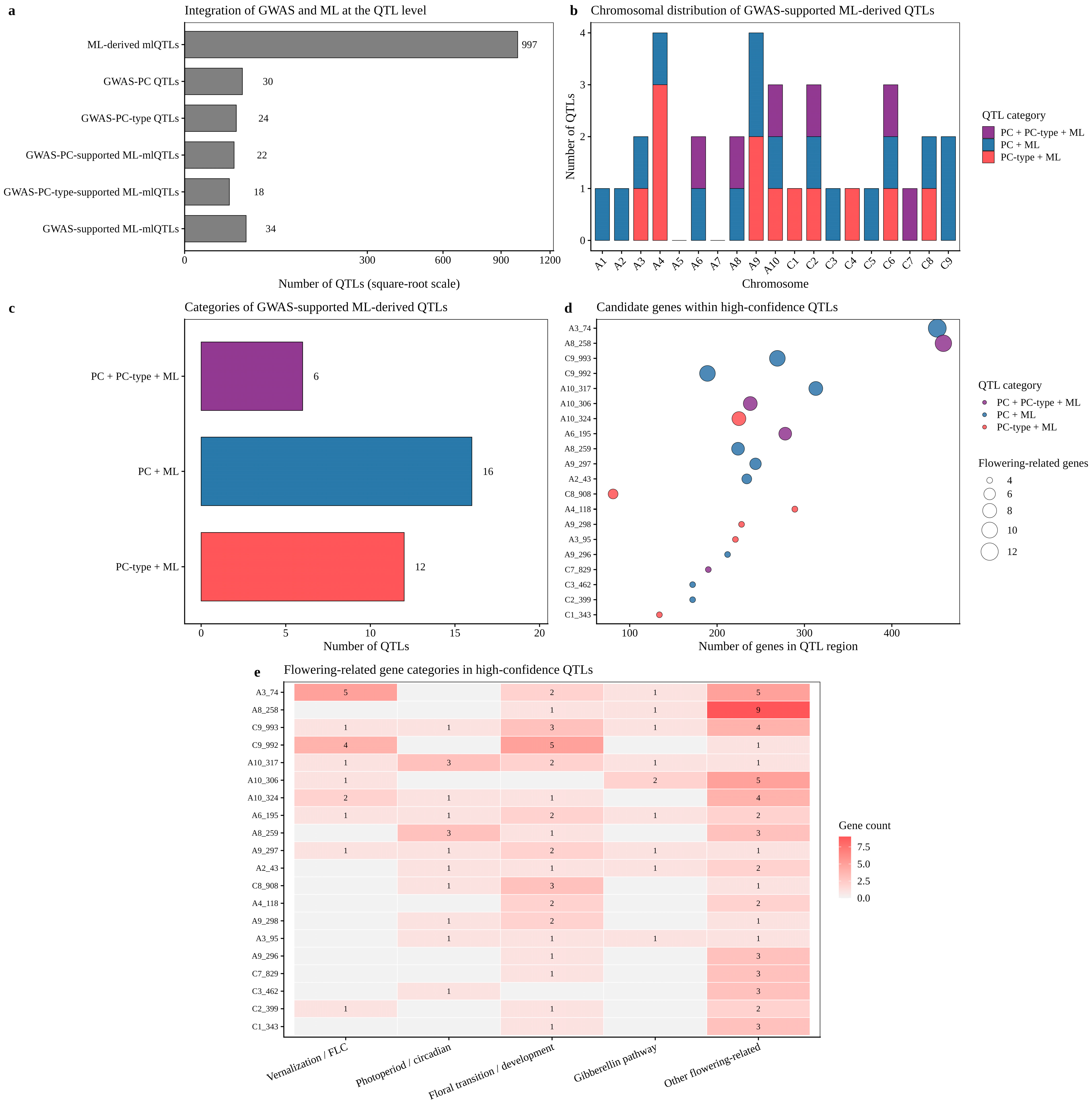
Because GWAS and machine learning may identify different representative SNPs within the same genetic region, direct comparison based on SNP-level overlap may underestimate the concordance between the two approaches. A single SNP often serves only as a linked marker for an underlying functional variant, and neighboring SNPs may collectively represent the same genetic-effect interval. Therefore, in this study, GWAS-suggestive SNPs and ML_delta10SD high-contribution SNPs were further merged into GWAS-derived QTLs and ML-derived ML-QTLs according to their physical positions, and the two types of intervals were integrated at the QTL level. The 32 suggestive SNPs identified by the FarmCPU-PC model were merged into 30 GWAS-derived QTLs, whereas the 27 suggestive SNPs identified by the FarmCPU-PC-Type model were merged into 24 GWAS-derived QTLs. In parallel, the 18,854 ML_delta10SD SNPs were merged into 997 ML-derived ML-QTLs. Through interval-level overlap comparison, 34 GWAS-supported ML-derived QTLs were finally identified. Among them, six QTLs were jointly supported by both GWAS models and machine learning, suggesting that these regions had relatively strong multi-source support.

These results indicate that integrating GWAS-based statistical association evidence with machine learning-based predictive contribution evidence at the QTL-interval level can more effectively prioritize high-confidence candidate regions. Compared with single-SNP overlap analysis, interval-level integration better reflects the regional nature of genetic signals and provides a more biologically meaningful framework for candidate QTL identification in complex traits such as flowering time. Nevertheless, these candidate regions should be regarded as prioritized genomic intervals rather than validated causal QTLs, and further validation is required to confirm their functional relevance.

4.5. Candidate Genes Within GWAS- and ML-Supported Candidate Regions Are Consistent with Known Flowering Regulatory Pathways

Candidate gene annotation showed that multiple GWAS-supported ML-derived QTL intervals contained genes known or predicted to be involved in flowering-time regulation, including FLC, FRIGIDA-like, VIN3-like, SOC1, ELF3, CONSTANS-like, APETALA1-like, and genes related to the gibberellin pathway. These genes are involved in several flowering regulatory pathways, such as vernalization, photoperiod response, circadian rhythm, flowering pathway integration, floral meristem formation, and hormone signaling. Among these genes, FLC is a central floral repressor in the vernalization pathway, and FRIGIDA can influence FLC expression and thereby regulate vernalization requirement and flowering time [12]. VIN3 is associated with vernalization-induced silencing of FLC, whereas SOC1 acts as an integrator of multiple flowering pathways [39,40]. In addition, ELF3 and CONSTANS-like genes are closely related to circadian rhythm and photoperiod response [41]. The detection of these flowering-related genes within high-confidence candidate regions indicates that the QTLs prioritized by integrating GWAS and machine learning have a plausible biological basis.

Furthermore, top-SNP genotypic effect analysis and multi-SNP genotype combination analysis showed that different genotypes in representative candidate QTLs were closely associated with flowering-time differences and the distribution of vernalization types. These results provide further support for the association between these candidate regions and flowering-time variation in B. napus. However, because independent population validation and functional experiments were not included in this study, these genes should be considered putative candidate genes rather than confirmed causal genes.

4.6. Limitations and Future Perspectives

Although this study integrated GWAS and machine learning to prioritize candidate regions associated with flowering time and vernalization-type differentiation in B. napus, several limitations should be acknowledged. First, the identified candidate regions and putative candidate genes were not validated using independent populations or functional experiments. Therefore, they should not be interpreted as confirmed causal loci. Second, the block-wise ExtraTreesRegressor strategy enabled genome-wide feature contribution screening under a large SNP matrix, but feature importance values across different SNP blocks may not be strictly comparable. Third, the prediction analysis was conducted within the present population, and its performance may be partly influenced by population structure and vernalization-type differentiation.

Future studies should validate these GWAS- and ML-supported candidate regions using independent populations, multi-environment field trials, transcriptomic data, eQTL analysis, gene editing, and other functional experiments. Such validation will be necessary to confirm causal genes, clarify regulatory mechanisms, and evaluate the breeding utility of candidate markers for flowering-time improvement and regional adaptation in rapeseed.

5. Conclusions

In this study, flowering time in B. napus was investigated by integrating genome-wide SNPs, phenotypic data, vernalization type, and geographic origin information. A genetic dissection framework combining FarmCPU-GWAS and machine learning-based feature contribution analysis was established. The results show that flowering time exhibited continuous variation in the natural B. napus population and was closely associated with differentiation among spring, semi-winter, and winter vernalization types. Differences in association signals detected by the two FarmCPU covariate models indicated that correction for vernalization type affected the identification of flowering-time-associated loci. Machine learning analysis identified 18,854 ML_delta10SD high-contribution SNPs. By integrating GWAS-derived QTLs and ML-derived ML-QTLs at the interval level, 34 GWAS-supported ML-derived QTLs were identified. Several high-confidence regions contained flowering-related candidate genes, including FLC, FRIGIDA-like, VIN3-like, SOC1, ELF3, CONSTANS-like, APETALA1-like, and genes related to the gibberellin pathway. These genes are involved in multiple flowering regulatory pathways, including vernalization, photoperiod response, circadian rhythm, flowering pathway integration, and hormone signaling. Further top-SNP genotypic effect analysis and multi-SNP genotype combination analysis supported the association of these candidate regions with flowering-time variation and vernalization-type differentiation. Overall, this study supports the complementary value of GWAS and machine learning for prioritizing candidate genomic regions associated with complex traits and provides candidate regions, putative candidate genes, and marker resources for future marker development, independent validation, functional characterization, and adaptive improvement in B. napus. However, these candidate regions and genes should not be interpreted as confirmed causal loci, and their biological functions and breeding utility require further validation using independent populations, multi-environment trials, and functional experiments.