Coupled Simulation of Greenhouse Crop Growth and Soil CO₂ Emissions Under Variable Irrigation Levels

Abstract

How to achieve the goal of water–carbon synergistic optimization in greenhouse crop production under water-saving irrigation strategies constitutes a key pathway for the development of protected agriculture. Our study takes muskmelon and tomato with drip irrigation in greenhouses as an example and establishes different irrigation levels based on cumulative surface evaporation (E_p) from a 20 cm pan. Here, four irrigation amounts (0.6 E_p, 0.8 E_p, 1.0 E_p, and 1.2 E_p) were set for muskmelon, and three irrigation amounts (0.5 E_p, 0.7 E_p, and 0.9 E_p) were set for tomato, and then a two-year fixed-site field experiment was conducted. The growth rates of both crops were significantly higher under full-water-supply treatments (M1.0 and M1.2 for muskmelon, T0.9 for tomato) than under water-deficient treatments (M0.8 and M0.6 for muskmelon, T0.5 for tomato) (p < 0.05) at the flowering stage, while the opposite was true at the harvesting stage. More than 85% of root systems were distributed in the soil layer, ranging from 0 to 40 cm, and the average RLD under M1.0 and T0.9 was significantly higher than that under other treatments by 14.3%~27.6% (p < 0.05). Muskmelon yields at 1.0 E_p were 22.9%~45.7% higher than those at 0.6 E_p and 0.8 E_p, while tomato yields peaked at 0.9 E_p and were 17.0%~19.4% higher than those under the other two treatments. Daily average soil CO₂ emission fluxes of muskmelon under M1.2 were 9.2%~32.2% higher than those of other treatments respectively, and that of tomato under T0.9 was more than 20% higher than under T0.7 and T0.5 treatments, respectively. The WHCNS-Veg model demonstrated excellent performance in simulating SWC, LAI, and soil CO₂ emission fluxes. The RMSE for SWC simulation ranged from 0.013 to 0.022 cm³·cm⁻³, for LAI simulation, it varied from 0.103 to 0.210 cm²·cm⁻², and for soil CO₂ emission flux simulation, it changed from 1.057 to 2.188 kg·hm⁻². It should be noted that the performance was higher under high irrigation levels than under water deficit levels. These results can provide a scientific basis for optimizing greenhouse irrigation schedules and regulating water–carbon synergy under different water resource conditions.

1. Introduction

Under the dual constraints of intensified global climate change and scarce cultivated land resources, greenhouses, as the core carrier of controlled agriculture, can effectively break through natural constraints by precisely regulating indoor environmental factors [1]. This significantly improves crop yield and quality, providing an important guarantee for the safe production of grains and vegetables [2]. Irrigation is a key regulatory measure in greenhouse crop production, and reasonable water supply serves as the core prerequisite for increasing crop yield and improving quality, while imbalanced irrigation amounts can indirectly regulate soil CO₂ emission intensity by altering key processes such as soil organic matter mineralization rates, microbial activity, root biomass, and gas diffusion efficiency in soil pores [3,4]. Currently, with the increasingly prominent contradictions between global warming and water resource supply and demand, how to achieve the goals of water conservation and emission reduction while ensuring greenhouse crop yield has become an important issue for alleviating global warming and promoting the sustainable development of protected agriculture.

As is well known, irrigation is the sole pathway of water input for greenhouse crops [5]. As a core carrier for photosynthesis and nutrient absorption, water supply levels directly regulate crop growth and development through soil moisture status [6]. On the one hand, soil water can significantly affect morphological indicators such as crop root density and distribution depth, thereby regulating photosynthetic efficiency and dry matter accumulation and ultimately acting on yield formation and quality characteristics (e.g., fruit sugar content and vitamin C content) [7]. On the other hand, soil water is also a key regulatory factor of the crop rhizosphere environment. Existing studies have confirmed that excessively high soil water content (SWC) inhibits root growth and reduces root physiological vitality, while excessively low SWC accelerates root senescence, impairs water absorption efficiency, and ultimately hinders root proliferation [6,8,9]. Hu et al. [7] also pointed out that deficit irrigation inhibits tomato root systems by reducing soil water availability, while over-irrigation deteriorates rhizosphere aeration conditions and restricts root expansion. Additional studies have shown that mild water stress promotes deep root growth, which is conducive to enhancing crop resource acquisition capacity [10]. Soil water is also a core environmental factor regulating crop photosynthesis, which acts on the photosynthetic process through multiple dimensions such as stomatal behavior, physiological metabolism, and morphological structure. Moreover, the influence mechanisms and effects of different irrigation levels (deficit, suitable, excessive) vary significantly [11]. Specifically, under mild water deficit (relative SWC 60%~70%), photosynthesis is mainly limited by leaf stoma, where stomatal conductance decreases by 10%~30% and net photosynthetic rate decreases by 5%~20% [12]. However, mild stress may improve WUE by regulating photosynthate distribution. Under moderate water deficit (relative SWC 45%~60%), photosynthesis is jointly affected by stomatal and non-stomatal limitations, where net photosynthetic rate decreases by 20%~50% [13]. Under severe water deficit (relative SWC < 45%), photosynthesis is dominated by non-stoma limitations, and net photosynthetic rate decreases by more than 50% or even approaches 0 [14]. The photosynthetic and growth responses ultimately affect yield components and quality indicators by regulating crop development, metabolism, and resource allocation processes. Studies have shown that when the lower limit of suitable SWC for greenhouse muskmelon is set at 65%~70% field capacity (θ_f), the fruit yield and quality are optimal [15]. When using the cumulative evaporation of the evaporating pan (E_p) as the basis for an irrigation plan, irrigation amounts of greenhouse cucumber during the developmental stage and mid-late growth stage should be controlled at 0.8 E_p and 1.2 E_p, respectively [16]. The lower limit of SWC for greenhouse pepper is 70% θ_f, and the lower limits of SWC for greenhouse tomato at the flowering and fruiting stages are 89.5% θ_f and 77.0% θ_f, respectively, to obtain the maximum yields and WUE [17]. Considering the fruit morphological indicators (e.g., single fruit weight, harvest index) and commercial yield of greenhouse tomato comprehensively, the optimal irrigation amount is 85.0% ET [18]. Although existing studies have clarified the regulatory effects of water on greenhouse crop growth, photosynthesis, and production efficiency, the differences in the effects of SWC on crop physiological growth and yields under different types of crops still need further in-depth research.

Agricultural soil is the primary source of global greenhouse gas emissions. Previous studies estimated that approximately 20% of atmospheric CO₂ comes from soils each year [19]. As an important part of the farmland ecosystem, protected vegetable fields have considerable contributions to greenhouse gas emissions due to characteristics such as large fertilizer applications and synchronous applications of water and fertilizer during cultivation. Therefore, the study of soil CO₂ emissions from protected vegetable fields has become a core content of energy conservation and emission reduction in the farmland ecosystem. Existing studies generally believe that SWC is a key driving factor of greenhouse gas emissions and carbon cycles, and within a certain range, SWC has a significant correlation with greenhouse gas emissions [20,21,22]. Studies by Liu et al. [23] and Wang et al. [24] have shown that different irrigation amounts increase soil respiration, but the relationship between soil respiration and irrigation amounts is not linear. Generally, under water-deficit conditions, soil respiration is positively correlated with irrigation amount, while excessive irrigation inhibits soil respiration. Studies by Muhr et al. [25], Jabro et al. [26], and Sänger et al. [3] have also confirmed that high SWC reduces soil oxygen availability, thereby inhibiting soil respiration or having no significant impact. Furthermore, Ouma [4] conducted a pot experiment on the effects of different irrigation frequencies on soil respiration of mango rootstock seedlings in Kenya, and the results showed that higher irrigation frequencies lead to higher soil respiration. While Morugάn-Coronado et al. [27] studied farmland soil in Spain and pointed out that prolonged drought periods between two irrigations cause microbial death and nutrient accumulation. However, greenhouses are semi-enclosed structures where the internal environment has higher temperature and humidity, and no natural rainfall occurs, which renders soil CO₂ emissions controllable. First, elevated temperatures enhance the growth and activity of greenhouse crop roots, increasing the contribution ratio of rhizospheric autotrophic respiration. Second, higher temperatures boost the photosynthetic capacity of greenhouse crops, prompting them to secrete more easily decomposable organic matter into the rhizosphere. This provides sufficient carbon sources for soil microorganisms and forms a positive feedback loop of enhanced photosynthesis increased rhizospheric carbon sources—elevated microbial respiration [19]. Finally, the water supply for greenhouse crops is mainly dependent on irrigation, which reduces the abruptness of soil moisture increase [11]. This allows the “Birch effect” to be triggered at a predetermined level of water deficit, and the intensity and duration of this effect can be regulated by adjusting the irrigation amount and rehydration rate. In summary, the significant changes in SWC and their distribution caused by varying irrigation amounts are bound to exert a significant impact on soil CO₂ emissions, and the characteristics of CO₂ emissions inside greenhouses are distinctly different from those in outdoor fields. However, current research has mostly focused on the emission reduction effects of agricultural practices such as straw return, no-tillage and organic fertilizer applications [28], while few studies have investigated the characteristics of CO₂ emissions under different water conditions in greenhouses.

Soil–crop system models can effectively predict SWC dynamics and crop growth processes, and they have been widely applied to water and fertilizer optimization management of field crops [29,30]. However, models suitable for water–carbon synergistic management of protected vegetables are still relatively scarce. Currently models such as CENTURY, DAISY, and DNDC are widely used, but their applicability under different water conditions in greenhouses has not been verified, and they have obvious limitations [31]. Firstly, DNDC and DAISY were originally developed for field crop ecosystems, with their microclimate response functions calibrated for open-field conditions, and they fail to consider the effects of the semi-enclosed greenhouse environment (stable high temperature, high humidity, no natural rainfall) on the coupling of soil carbon cycles and crop growth. Secondly, the CENTURY model has an oversimplified organic carbon pool division and lacks a specialized root respiration simulation module adapted to the multi-growth stage characteristics of protected vegetable crops. (3) Finally, none of the three models incorporates a simulation sub-module for the Birch effect induced by drip irrigation rehydration, which is a key process of pulsed soil CO₂ emissions in greenhouses, leading to large errors in simulating soil CO₂ emission dynamics under different irrigation regimes [32]. Protected vegetables have the characteristics of multiple harvests, and the vegetable growth and development module in the EU_Rotate-N model can effectively adapt to this feature [33,34,35]. Therefore, our study draws on the vegetable growth and development module of the EU_Rotate-N model and couples it with the soil water movement and carbon cycles modules of the WHCNS model to construct a water–carbon management model suitable for protected vegetable fields in greenhouse environments.

Based on the aforementioned research results, our paper puts forward the following hypotheses: moderate-water-deficit irrigation can maintain a relatively high crop yields while reducing water consumptions and improving WUE; irrigation amounts can regulate the characteristics of greenhouse soil CO₂ emissions by altering the dynamics of SWC; and calibration of the parameters for the semi-enclosed greenhouse environment can enhance the performance of the WHCNS-Veg model. To address these issues, the objectives were to: (1) investigate the growth rates, root length density, yields, and water consumption of greenhouse muskmelons and tomatoes under different irrigation levels; (2) calibrate the model parameters of WHCNS-Veg to make it more suitable for the greenhouse environment; and (3) simulate the LAI, SWC, and soil CO₂ emissions using the improved WHCNS-Veg model.

2. Materials and Methods

2.1. Experiment Site

The experiment was conducted in greenhouses at the Agricultural High-Efficiency Water Use Experimental Base in Henan Province (34°47′ N, 113°47′ E, elevation 81.2 m) from February to June in 2023 and 2024. The experimental area belongs to a warm temperate continental monsoon climate zone, with an average annual rainfall of 551 mm, an average annual evaporation of 1911 mm, a multi-year average temperature of 14.1 °C, an annual sunshine duration of 2401 h, and a frost-free period of 201 days. The soil in the greenhouses is loam. The average bulk density, field capacity, and wilting point SWC of the 0–60 cm soil layer are 1.51 g·cm⁻³, 0.366 cm³·cm⁻³, and 0.09 cm³·cm⁻³, respectively. Detailed soil physical and chemical properties can be found in

Table 1. Soil physical and hydraulic properties for soil profile in the greenhouse.

Depth/cm	BD/(g·cm−3)	θr/(cm3·cm−3)	θs/(cm3·cm−3)	α/(cm−1)	n	Ks/(cm·d−1)
0–20	1.49	0.032	0.373	0.0079	1.282	3.5
20–40	1.51	0.025	0.430	0.0094	1.294	4.1
40–60	1.48	0.029	0.366	0.0072	1.280	3.4

BD is the soil bulk density; θ_r is the residual water content; θ_s is the saturated water content; α is the inverse of the air-entry value; n is a pore size distribution index; K_s is the saturated hydraulic conductivity.

.

2.2. Experiment Design

This experiment was conducted in two identical greenhouses using muskmelon (cv. Hongmi 17) and tomato (cv. Jinpeng M6). Each greenhouse had the same type and area (340 m², 40 m × 8.5 m), oriented east–west, with a steel frame structure. The roof of each greenhouse was covered with a 0.2 mm thick polyethylene film, over which a quilt layer was laid primarily for heat preservation, particularly during the seedling stage. Each greenhouse was equipped with three vents (top, south, and north) for temperature regulation and air circulation.

Muskmelons were transplanted on 15 April 2023 and 12 April 2024. A wide–narrow row planting pattern was adopted, with wide rows of 70 cm, narrow rows of 40 cm, and a plant spacing of 30 cm. Harvesting started on 18 June and concluded on 25 June. Tomatoes were transplanted on 10 March 2023 and 12 March 2024. Harvesting began on 1 June and ended on 28 June. The same planting pattern was used, with wide rows of 65 cm, narrow rows of 45 cm, and a plant spacing of 30 cm.

The drip irrigation method was employed for water supply. Rotary water meters with an accuracy of 0.001 m³ were installed on the pipelines of each plot. Netafim pressure-compensating drip tapes were laid along the crop rows in each plot, with a dripper spacing of 30 cm, a rated dripper flow rate of 1.1 L·h⁻¹, and an operating pressure of 0.1 MPa. Entering the fruiting stage, 16 kg·hm⁻² urea and 24 kg·hm⁻² potassium sulfate was topdressed. During the whole growth period, muskmelons and tomatoes were topdressed three and four times, respectively. Irrigation frequency and amount were determined with reference to the cumulative water surface evaporation (E_p) of a 20 cm standard evaporation pan. The evaporation pan was placed 30 cm above the crop canopy and adjusted with plant height. Water surface evaporation of the previous day was measured at 7:00 am daily using a rain gauge. After measurement, the interior of the evaporation pan was cleaned, and tap water was added to a depth of 20 mm. For loam soil with a bulk density ranging from 1.45 to 1.55 g·cm⁻³, an irrigation schedule can be adopted where irrigation is implemented when the cumulative surface evaporation reaches 18 ± 2 mm. In this study, four evaporation pan coefficients were set (0.6, 0.8, 1.0, and 1.2) for muskmelons and three evaporation pan coefficients were set (0.5, 0.7, and 0.9) for tomatoes. Each treatment had three replicates and was arranged in a randomized block design. Detailed experimental treatments are shown in

Table 2. Watering standards for muskmelon and tomato under different treatments.

Crops	Treatments	Seedling	From Flowering to Harvesting
Muskmelon	M0.6	25 mm + 1.0 Ep	0.6 Ep
	M0.8	25 mm + 1.0 Ep	0.8 Ep
	M1.0	25 mm + 1.0 Ep	1.0 Ep
	M1.2	25 mm + 1.0 Ep	1.2 Ep
Tomato	T0.5	20 mm + 1.0 Ep	0.5 Ep
	T0.7	20 mm + 1.0 Ep	0.7 Ep
	T0.9	20 mm + 1.0 Ep	0.9 Ep

The seedling period of muskmelon was from 15 April 2023 to 4 May 2023 and from 12 April 2024 to 1 May 2024. The flowering and fruiting period was from 5 May 2023 to 17 June 2023 and from 2 May 2024 to 17 June 2024. The harvest period was from 18 June 2023 to 28 June 2023 and from 18 June 2024 to 25 June 2024. The seedling period of tomato was from 10 March 2023 to 5 April 2023 and from 12 March 2024 to 7 April 2024. The flowering and fruiting period was from 6 April 2023 to 31 May 2023 and from 8 April 2024 to 31 May 2024. The harvest period was from 1 June 2023 to 28 June 2023 and from 1 June 2024 to 30 June 2024.

.

2.3. Measurements

2.3.1. Meteorological Factors in the Greenhouse

An automatic meteorological monitoring system was installed in the center of each greenhouse, including sensors for solar radiation (R_s), relative humidity (RH), air temperature (T_a), and wind speed (u), which were placed at a height of 2 m above the ground surface. R_s was measured using a radiometer (LI200X, Campbell Scientific, Inc., Logan, UT, USA) with an accuracy of 0.2 kW m⁻²(mV)⁻¹. T_a and RH were determined by a temperature and humidity recorder (CS215, Campbell Scientific, Inc., Logan, UT, USA). Wind speed was measured with an anemometer (Wind Sonic, Gill, UK) with an accuracy of 0.02 m s⁻¹. All data were recorded every 10 s, averaged every 30 min, and stored in a CR1000 data logger (Campbell Scientific Inc., Logan, UT, USA).

A 20 cm standard evaporation pan (ADM 7) was used to measure the water surface evaporation at 30 cm above the crop canopy. Water surface evaporation of the previous day was measured at 7:00 am daily using a rain gauge with an accuracy of 0.1 mm. After each measurement, the pan was refilled with 20 mm of clean water.

2.3.2. Soil Water Content and Temperature in the Root Zone

Soil water content (SWC) in the 0–60 cm layer was measured by using the oven-drying method. Before each irrigation, soil samples were collected at 10 cm intervals using a soil auger, then placed in aluminum boxes, and immediately weighed for wet mass. After all samples were collected, they were dried in an oven at 105 °C to reach constant mass. Sampling points were selected at the midpoint between two drippers of the drip tape, with three replicates per plot.

Soil temperatures at 0, 5, 10, and 20 cm in the root zone were measured using soil temperature meters with an accuracy of 0.2 °C. Data were automatically collected every hour and stored in JL–04 data loggers.

2.3.3. Plant Growth and Root Length Density

Plant height and leaf area were observed every 5–10 days. Plant height was measured with a ruler, and leaf area was calculated as follows: a leaf area conversion coefficient was obtained through multiple fittings between CAD technology and direct measurement results. Leaf area = maximum leaf length × maximum leaf width × conversion coefficient. Leaf area index (LAI) is the ratio of total leaf area to the unit surface area. Through CAD fitting, the leaf area conversion coefficients for muskmelon and tomato were 0.728 and 0.685, respectively.

Root length density (RLD) in the 0–60 cm root zone was measured using the layered sampling method with a root auger at 10 cm intervals down to the maximum root penetration depth. Collected root samples were cleaned using water, and root images were acquired using an EPSON scanner. RLD was calculated using the WinRHIZO root analysis system (WinRHIZO Pro2004b, Régent Instruments Inc., Guelph, ON, Canada).

2.3.4. Yield, Water Consumption, and Water Use Efficiency

For muskmelon management, only one fruit was retained per plant, and the final yield was the total yield from all harvest. For each treatment, 20 plants at the middle position of the plot were marked for measurement. The single fruit weight in each plot was weighed using an electronic balance with an accuracy of 5 g, and the final yield of each plot was calculated. For tomato management, 20 plants were also fixed at the middle position of each replicate plot, and the yield of 60 plants per treatment was measured. Yield was determined individually using an electronic balance with an accuracy of 5 g, and single fruit weight was measured with an electronic balance with an accuracy of 0.01 g.

Water consumption (ET) of each plot was calculated using the water balance method, and the formula is as follows:

ET = P + I + U − D + (W₀ − W_t)

(1)

where ET is the water consumption (mm); P is the precipitation (mm); I_r is the total irrigation amount (mm); U is the groundwater recharge (mm); D is the deep percolation (mm); and W₀ and W_t are the soil water storage in the 0–60 cm soil layer at the beginning and end of the growth period (mm), respectively. In the greenhouse, there was no precipitation (P = 0). In addition, the groundwater level was below 5.0 m, which was unavailable for crop absorption, so groundwater recharge was negligible (U = 0). The drip irrigation amount was small, resulting in no deep percolation (D = 0).

Water use efficiency (WUE) refers to the dry matter produced per unit mass of water consumed by crop transpiration in the field. Irrigation water use efficiency (IWUE) denotes the percentage of total irrigation water introduced to the field that is effectively absorbed and utilized by crops. They can be calculated using the following formula:

WUE = Y/ET × 100

(2)

IWUE = Y/I_r × 100

(3)

where Y is the total fruit yield (kg·hm⁻²); I_r is the total irrigation amount (mm); and ET is the total water consumption (mm).

2.3.5. Soil CO₂ Emission Flux

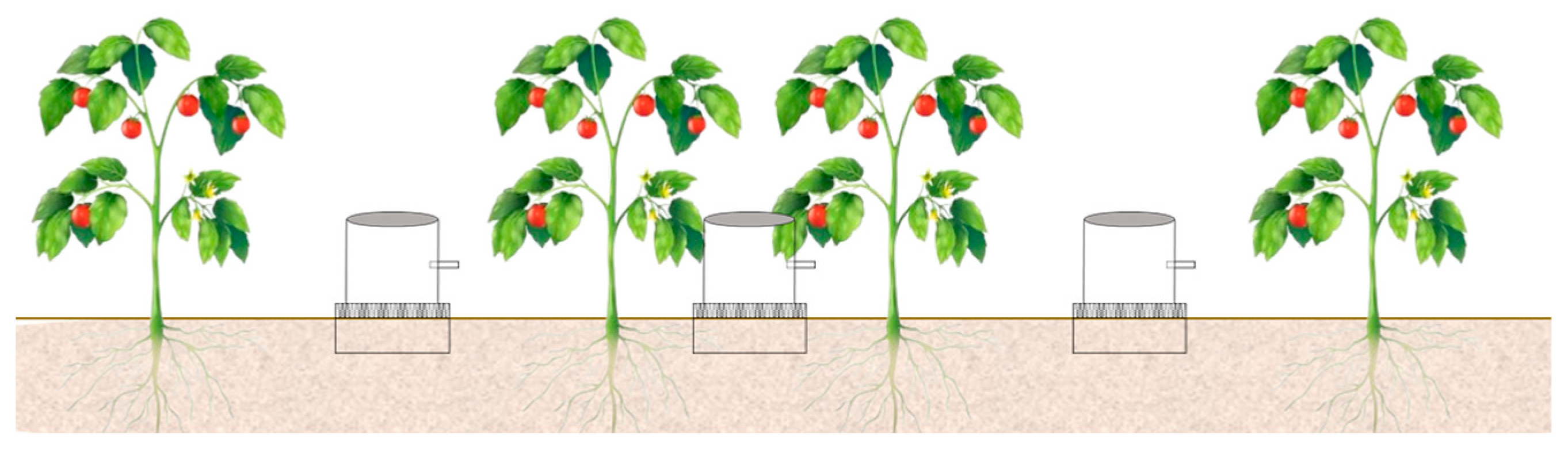
Soil CO₂ emission fluxes in the different treatments were measured using an SC8000 portable soil CO₂ analyzer, which consisted of an ELO105 data logger (LSI Lastem, Milan, Italy) and a GMM220 series CO₂ sensor (Vaisala, Vantaa, Finland). This system collected data every 30 min. Sampling chambers were made of large PVC pipes, with a diameter of 20 cm and a height of 40 cm. A 2.5 cm diameter PVC pipe extended outward from one side of the chamber (Figure 1). The chamber was wrapped with a reflective thermal insulation material (double-sided aluminum film composite bubble pad, aluminum film + EPE material) to prevent interference from the external temperature on the gas inside the chamber. Bases were buried at two positions (narrow and wide rows) and fixed during the experiment. For measurement, the sampling chamber was vertically placed in the groove of the base and sealed with water to ensure no gas exchange between the inside of the chamber and the atmosphere. Then, the probe was inserted into the chamber through the 2.5 cm PVC pipe and sealed with clay. Specifically, to ensure the consistency of measurement conditions and reduce the interference of diurnal air temperature variations on manual operations, on-site measurements were performed daily during two time windows: 8:00–10:00 and 15:00–17:00. Meanwhile, the ELO105 data logger equipped with the analyzer was set to automatically collect real-time data of CO₂ emission fluxes at 30 min intervals throughout the entire experimental period. This continuous and automatic data acquisition mode allowed for a complete recording of the dynamic changes in soil CO₂ emissions, including the short-term pulsed CO₂ emission peaks induced by the “Birch effect” after drip irrigation rehydration, effectively avoiding the underestimation of total emissions that would result from discontinuous weekly measurements.

2.4. WHCNS-Veg Model

The WHCNS-Veg coupled model mainly includes modules such as meteorological data, soil water movement, soil heat conduction, organic matter turnover, crop growth, carbon emission, and field management. The model adopts C++ object-oriented programming technology to organically integrate these modules, and each module can run independently or as a whole. In this study, the WHCNS-Veg model was calibrated by using field-measured data of SWC, LAI, and soil CO₂ emissions from M1.2 (muskmelon) and T0.9 (tomato) in 2023. Subsequently, the model was validated with measured data from other treatments in 2023 and all treatments in 2024.

2.4.1. Simulation of Soil Water Content

Surface runoff was calculated using the runoff curve number equation recommended by the United States Department of Agriculture (USDA) [36], and soil water infiltration was simulated using the Green-Ampt model [37]:

$$f=K_s\left(1+{\displaystyle \frac{h_f\Delta \theta }{F}}\right)$$

(4)

where f is the infiltration rate (cm·d⁻¹); K_s is the saturated hydraulic conductivity of soil (cm·d⁻¹); F is the cumulative infiltration (cm); h_f is the matric potential at the wetting front (cm); and Δθ is the difference between saturated SWC and initial SWC (cm³·cm⁻³).

The re-distribution of SWC also employed the Richards equation.

$${\displaystyle \frac{\mathsf{\partial }\theta }{\mathsf{\partial }t}}={\displaystyle \frac{\mathsf{\partial }}{\mathsf{\partial }z}}\left[k\left(h\right)\left({\displaystyle \frac{\mathsf{\partial }h}{\mathsf{\partial }z}}+1\right)\right]-S_w$$

(5)

$$h\left(z,t\right)=h_i\left(z\right)t=0,0\le z\le L$$

(6)

$$\left|-k\left(h\right){\displaystyle \frac{\mathsf{\partial }h}{\mathsf{\partial }z}}-k\left(h\right)\right|\le E_{p}t>0, z=L, h_A\le h\le 0$$

(7)

where h is the soil matric potential (cm); θ is the volumetric SWC (cm³·cm⁻³); t is the time (d); z is the spatial coordinate (positive upward), (cm); L is the distance from the lower boundary to the upper boundary (cm); k(h) is the unsaturated hydraulic conductivity (cm·d⁻¹); S_w is the root water uptake term (cm³·cm⁻³·d); h_i is the initial soil matric potential at different positions (cm); E_p is the potential evaporation under current atmospheric conditions (cm·d⁻¹); and h_A is the minimum allowable matric potential at the soil surface (cm). When the groundwater table in the study area was deeply buried, the lower boundary was set as a free drainage boundary:

$${\displaystyle \frac{\mathsf{\partial }h}{\mathsf{\partial }z}}=0t\ge 0,z=0$$

(8)

The reference crop evapotranspiration (ET₀, cm·d⁻¹) was calculated by using the Penman–Monteith equation recommended by the Food and Agriculture Organization of the United Nations (FAO) [38]. Subsequently, the crop evapotranspiration (ET, cm·d⁻¹) was computed by using the crop coefficient (K_c). Furthermore, combined with LAI, the potential evaporation (E_p, cm·d⁻¹) and potential transpiration (T_p, cm·d⁻¹) of actual crops were derived [39], as detailed below:

$$ET=E{T}_0\times K_c$$

(9)

$$E_p=\left\{\begin{array}{l}ET\times \exp \left(-0.4\times LAI\right)/1.1LAI>1.0\\ ET\times \left(1-0.43\times LAI\right) 0<LAI\le 1.0\end{array}\right.$$

(10)

$$T_p=ET-E_p$$

(11)

2.4.2. Simulation of Leaf Area Index

The Dutch PS123 model was incorporated into the WHCNS-Veg model for simulating crop LAI [40]. LAI is related to temperature, light intensity, and the crop’s Relative Development Stage (RDS). Many scholars have used specific leaf area (SLA, m²·kg⁻¹) to calculate LAI, arguing that SLA is maximum at emergence (SLA_max), then decreases linearly, and reaches a minimum at crop maturity (SLA_min). The calculation formula is as follows:

$$SLA=\left\{\begin{array}{c}SL{A}_{min}-\left(SL{A}_{max}-SL{A}_{min}\right)\times \ln \left(RDS\right) SLA\le SL{A}_{max}\hfill \\ \hfill SL{A}_{max} SLA>SL{A}_{max}\end{array}\right.$$

(12)

$$LAI=livS\left(leaf\right)\times SLA\times {10}^{-4}$$

(13)

where livS(leaf) is the live leaf dry matter weight.

2.4.3. Simulation of Soil CO₂ Emissions

The WHCNS-Veg model explicitly distinguishes between root respiration (autotrophic respiration) and microbial respiration (heterotrophic respiration) in its soil carbon cycle module and quantifies these two components independently before integrating them to simulate the total ground respiration of the greenhouse soil–crop system. This total ground respiration is the core object of soil CO₂ emission simulation in our study. The WHCNS-Veg model embeds the Dutch Daisy module, which classifies organic matter into three main pools: added organic matter (AOM) pool, soil organic matter (SOM) pool, and soil microbial biomass (SMB) pool. Each main pool is further divided into two sub-pools: a slowly decomposable pool (AOM₁, BOM₁, and SOM₁) and a rapidly decomposable pool (AOM₂, BOM₂, and SOM₂), with each sub-pool having a specific carbon-to-nitrogen (C/N) ratio. The decomposition of each organic matter pool or microbial mortality is described by a first-order kinetic equation:

$${\xi }_p=k_p\cdot C_p$$

(14)

where ζ_p is the decomposition amount of the p_-th organic matter pool or microbial mortality per unit time (kg·m⁻³·s⁻¹, based on C); C_p is the carbon content of the p_-th organic matter pool (kg·m⁻³, based on C); and k_p is the decomposition rate constant of the p_-th organic matter pool or microbial mortality rate constant (d⁻¹). The AOM pool in soil can be calculated by using the following equation [32]:

$$k_{AOM}={k^{*}}_{AOM}{F}_m\left(T\right)F_m\left(h\right)$$

(15)

$$F_m\left(T\right)=\left\{\begin{array}{c}\hfill 0 T\le 20 \\ \hfill 0.1T 0<T\le 20\\ \exp \left(0.47-0.027T+0.00193T^2\right) T>20 \hfill \end{array}\right.$$

(16)

$$F_m\left(h\right)=\left\{\begin{array}{c}\hfill 0.6 h\ge -\left({10}^{-2}\right) \\ 0.6+0.4\log \left(-100h\right)/1.5 -\left({10}^{-2}\right)>h\ge -\left({10}^{-0.5}\right)\hfill \\ \hfill 1.0 -\left({10}^{-0.5}\right)>h\ge -\left({10}^{0.5}\right)\\ 1.0-\log \left(-100h\right)/4.0 -\left({10}^{0.5}\right)>h\ge -\left({10}^{4.5}\right)\hfill \\ \hfill 0 -\left({10}^{4.5}\right)>h \end{array}\right.$$

(17)

where k*_AOM is the maximum decomposition rate constant of exogenous organic matter by microorganisms under optimal moisture and temperature conditions (d⁻¹); T is the soil temperature (℃); h is the soil matric potential (cm); and F_m(T) and F_m(h) are temperature and moisture calibration functions, respectively.

For the SOM₁ and SOM₂ pools, the effect of clay content is considered in addition to moisture and temperature calibration:

$$K_{SOM}={k^{*}}_{SOM}{F}_m\left(Clay\right)F_m\left(T\right)F_m\left(h\right)$$

(18)

$$F_m\left(Clay\right)=\left\{\begin{array}{l}1.0-a{C}_c{ 0<C}_c\le C_c’\\ 1.0-a{C}_c’{ C}_c>C_c’\end{array}\right.$$

(19)

where k*_SOM is the maximum decomposition rate constant of organic matter by microorganisms under optimal moisture and temperature conditions (d⁻¹); F_m(Clay) is the soil clay content calibration function; C_c is the soil clay content (kg·kg⁻¹); and C_c’ and a are the empirical parameters, with values of 0.25 kg·kg⁻¹ and 0.02, respectively.

The decomposition process of the SMB pool consists of two parts: microbial mortality and microbial maintenance respiration, both of which are closely related to soil moisture and temperature:

$${k^{*}}_{SMB}=d^{*}+m^{*}$$

(20)

$$k_{SMB}={k^{*}}_{SMB}{F}_m\left(T\right)F_m\left(h\right)$$

(21)

where k*_SMB is the microbial mortality and maintenance respiration rate under optimal moisture and temperature conditions (d⁻¹); d* is the microbial mortality rate under optimal moisture and temperature conditions (d⁻¹); and m* is the microbial maintenance respiration rate under optimal moisture and temperature conditions (d⁻¹). After decomposition by microorganisms, AOM can be converted into SMB; upon SMB mortality, it can be further transformed into SOM, which can also be utilized by microorganisms and incorporated into the microbial biomass.

Hansen et al. [41] indicated that soil greenhouse gas emissions are closely related to nitrogen mineralization and immobilization processes and soil microbial activity, soil CO₂ emission directly originates from the decomposition of the SMB pool, there is a linear relationship between potential denitrification and soil CO₂ emission, and the mineralization and immobilization process is closely associated with the C/N ratio of soil organic matter:

$$S_{min}=-{\displaystyle \sum _{p=1}^6\frac{d{C}_p/dt}{{\left[C/N\right]}_p}}$$

(22)

where S_min is the organic matter mineralization rate (μg·cm⁻³·d⁻¹); C_p is the nitrogen content of the p_-th organic matter pool (kg·hm⁻², based on C); and [C/N]_p is the C/N ratio of the p_-th organic matter pool.

In this study, the WHCNS-Veg model not only distinguishes the two components of root respiration and microbial respiration and quantifies them separately, but also takes their sum as the simulation object of total ground respiration, which is consistent with the experimental measurement system and the research objective of exploring the response of greenhouse soil CO₂ emissions to different irrigation regimes in this study.

2.5. Model Evaluation

Two statistical indicators were used to evaluate the performance of the WHCNS-Veg model, namely the root mean square error (RMSE) and modeling efficiency (EF). The RMSE can describe the variance in errors in model estimation results, and the EF represents the ratio of the mean square error to the variance in the observed data. The calculation formulas are as follows:

$$RMSE={\left[{\displaystyle \frac{{\displaystyle {\sum }_{i=1}^n{\left(O_i-P_i\right)}^2}}{n}}\right]}^{0.5}$$

(23)

$$EF=1.0-{\displaystyle \frac{{\displaystyle {\sum }_{i=1}^n{\left(O_i-P_i\right)}^2}}{{\displaystyle {\sum }_{i=1}^n{\left(O_i-\overline{O}\right)}^2}}}$$

(24)

where O_i and P_i (i = 1, 2, …, n) are the measured and calculated values, $\overline{O}$ are the respective mean values, and n is the number of measurement values. A better model performance will have RMSE ≈ 0 and EF ≈ 1.0.

2.6. Statistical Analysis

All statistical analyses were conducted using SPSS 26.0 (IBM, Armonk, NY, USA). Before conducting the statistical analysis, the original data were preprocessed. The structure of this statistical model was designed based on the experimental design (randomized block design, including various drip irrigation treatments and repeated measurements), where fixed effects, random effects, and repeated factors were clearly distinguished. For different types of indicators, targeted statistical methods were adopted to ensure the rationality and reliability of the analysis results. Two-way analysis of variance (ANOVA) (treatment factor × year factor) was used to test the main effects of the treatment factor and the year factor on yield, WUE, and RLD, as well as their interaction effects.

For all parameter statistical analyses, strict hypothesis testing was conducted. After conducting the variance analysis, multiple comparisons were performed to test the pairwise differences among treatments. Duncan’s new multiple range test was used to evaluate yield and water use efficiency. The exact p-values of all statistical tests were reported (p < 0.05 was considered statistically significant, p < 0.01 was considered highly statistically significant).

3. Results

3.1. Meteorological Factors in the Greenhouse

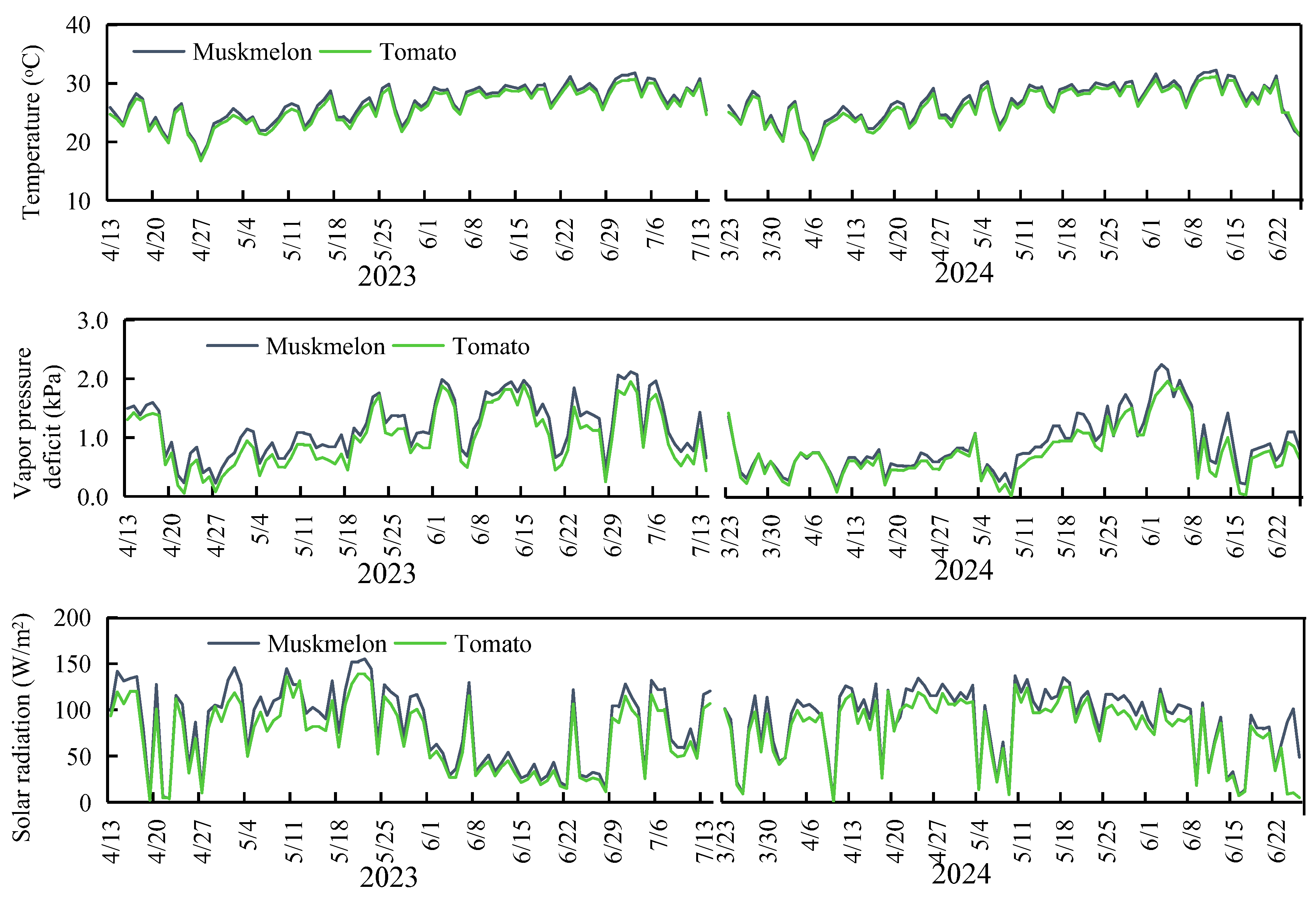
The dynamics of T_a, vapor pressure deficit (VPD), and R_s during the growth periods of muskmelon and tomato in 2023 and 2024 are presented in Figure 2. Notably, T_a exhibited minimal variability across the two study years, ranging from 12.0 to 32.7 °C, with average values of 25.4 °C (muskmelon) and 24.9 °C (tomato). The temperature difference between the two greenhouses was merely 0.5 ± 0.2 °C. In contrast, VPD and R_s displayed substantial fluctuations. Here, VPD varied from 0.02 to 2.20 kPa, with average values of 1.02 kPa (muskmelon) and 0.86 kPa (tomato), respectively; R_s ranged from 0.42 to 155.1 W·m⁻², with average values of 86.2 W·m⁻² (muskmelon) and 74.9 W·m⁻² (tomato), respectively. However, the inter-greenhouse differences in VPD and R_s were relatively small, at 0.16 ± 0.04 kPa and 11.3 ± 5.95 W·m⁻², respectively.

Furthermore, the mean values and standard deviations of meteorological factors at the seedling, flowering–fruiting, and harvesting stages of the two crops are summarized in

Table 3. The mean values and standard deviations of temperature (T_a), vapor pressure deficit (VPD), and solar radiation (R_s) at seedling, flowering–fruiting, and harvesting growth stages.

Stages	Factors	2023			2024
		Muskmelon	Tomato	Difference	Muskmelon	Tomato	Difference
Seedling	Ta	23.6 ± 2.7	23.0 ± 2.6	0.6 ± 0.2	19.2 ± 1.9	19.6 ± 2.1	0.4 ± 0.4
	VPD	0.89 ± 0.45	0.71 ± 0.46	0.18 ± 0.05	0.61 ± 0.25	0.58 ± 0.29	0.04 ± 0.03
	Rs	90.3 ± 47.5	77.2 ± 40.8	13.1 ± 9.1	77.9 ± 32.0	69.2 ± 27.7	8.8 ± 5.8
Flowering –fruiting	Ta	26.5 ± 2.4	25.8 ± 2.4	0.7 ± 0.2	23.5 ± 3.2	23.2 ± 3.1	0.4 ± 0.3
	VPD	1.26 ± 0.42	1.09 ± 0.45	0.17 ± 0.06	0.79 ± 0.36	0.68 ± 0.33	0.11 ± 0.08
	Rs	88.6 ± 41.2	76.5 ± 36.9	12.3 ± 6.4	99.6 ± 32.2	90.0 ± 29.4	10.0 ± 5.3
Harvesting	Ta	29.1 ± 1.8	28.4 ± 1.7	0.7 ± 0.3	28.4 ± 2.2	27.7 ± 2.2	0.7 ± 0.2
	VPD	1.31 ± 0.50	1.08 ± 0.48	0.23 ± 0.04	1.12 ± 0.57	0.93 ± 0.56	0.20 ± 0.09
	Rs	70.5 ± 41.6	60.4 ± 36.5	10.2 ± 6.2	70.5 ± 32.1	56.7 ± 33.4	13.9 ± 21.6
Whole stages	Ta	26.6 ± 2.5	25.9 ± 2.6	0.7 ± 0.2	24.1 ± 2.0	23.8 ± 2.2	0.3 ± 0.2
	VPD	1.19 ± 0.32	1.0 ± 0.41	0.19 ± 0.04	0.85 ± 0.35	0.73 ± 0.31	0.12 ± 0.03
	Rs	83.8 ± 38.5	72.0 ± 41.2	11.8 ± 7.2	88.7 ± 35.4	77.9 ± 33.6	10.8 ± 4.7

. It is evident that the average T_a inside the greenhouses was relatively low at the seedling stage, slightly increased at the flowering–fruiting stage, and peaked at the harvesting stage, with negligible T_a differences between the two crops across the two greenhouses. Similarly, VPD was smaller at the seedling stage but showed no significant disparity between the flowering–fruiting stages and the harvesting stages. This phenomenon is attributed to the low outdoor T_a during the seedling stage, where ventilation vents were closed to elevate the greenhouse internal temperature, leading to increased relative humidity and thus a subsequent decrease in VPD. Unlike T_a and VPD, although the outdoor R_s was relatively high in June, the internal R_s of the greenhouses did not follow this trend. This discrepancy may be ascribed to shading measures implemented to reduce the internal greenhouse temperature. It is worth noting that R_s exhibited a large amplitude of variation, with the inter-greenhouse difference fluctuating around 10 W·m⁻², indicating that R_s exhibited lower controllability relative to T_a and VPD in greenhouse environments.

3.2. Plant Growth Rate and Root Length Density

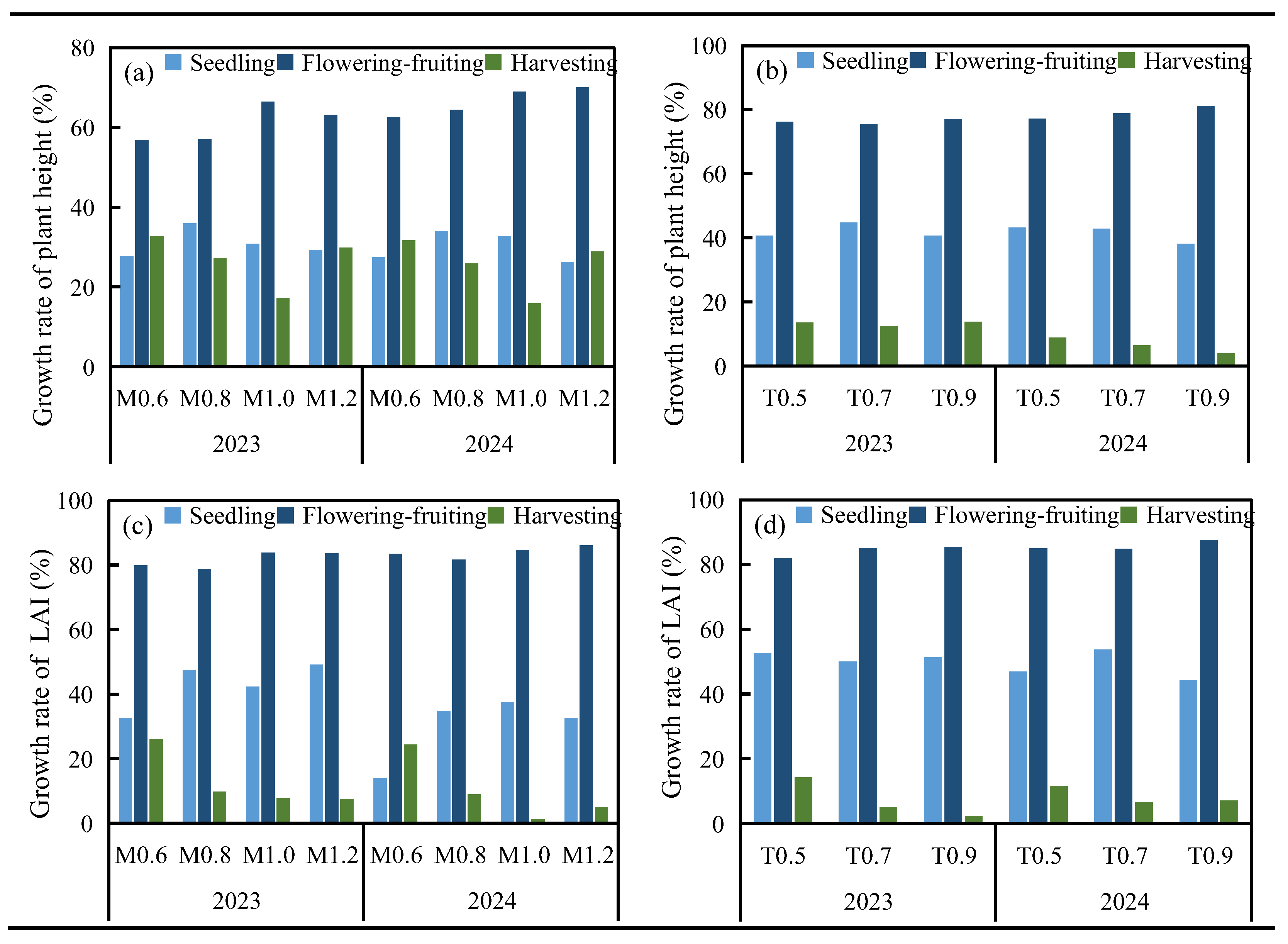
Figure 3 illustrates the growth rates of muskmelon and tomato at different growth stages under varying water conditions. The growth rate showed little difference at the seedling stage, peaked at the flowering–fruiting stage, and was lowest (even approaching zero) at the harvesting stage. This phenomenon is attributed to the similar water conditions at the seedling stage and the topping of the crops at the harvesting stage. For muskmelon, at the flowering–fruiting stage, the growth rates of plant height and LAI in M1.0 and M1.2 were significantly higher than those in M0.6 and M0.8. Specifically, growth rates of plant height and LAI in M1.0 were 11.3% and 4.7% higher than those in M0.6 and M0.8, respectively. In contrast, the trend at the harvesting stage was distinctly opposite. Growth rates of plant height and LAI in M1.0 and M1.2 were significantly lower than those in M0.6 and M0.8, with M1.0 showing decreases of 48.5% and 82.5% compared to those in M0.6 and M0.8, respectively. It is evident that the high-water treatments did not necessarily promote muskmelon growth in the greenhouse. For greenhouse-grown tomato, there was no significant difference in growth rates among the different water treatments at the flowering–fruiting stage. Plant height growth rate ranged from 75.6% to 81.2%, with a maximum difference of only 4.9% in plant height growth rate (between T0.5 and T0.9 in 2024). LAI growth rate varied from 81.9% to 87.6%, with a maximum difference of merely 4.2% in LAI growth rate (between T0.5 and T0.9 in 2023). At the harvesting stage, growth rate of T0.5 was significantly higher than in T0.9. Growth rates of plant height and LAI in T0.5 were 27.3% and 61.4% higher than those in T0.9, respectively. Although the T0.9 water treatment did not substantially enhance the plant growth rates, it facilitated plant reproductive growth by increasing the number of flowers, which was prominently reflected in the final yield.

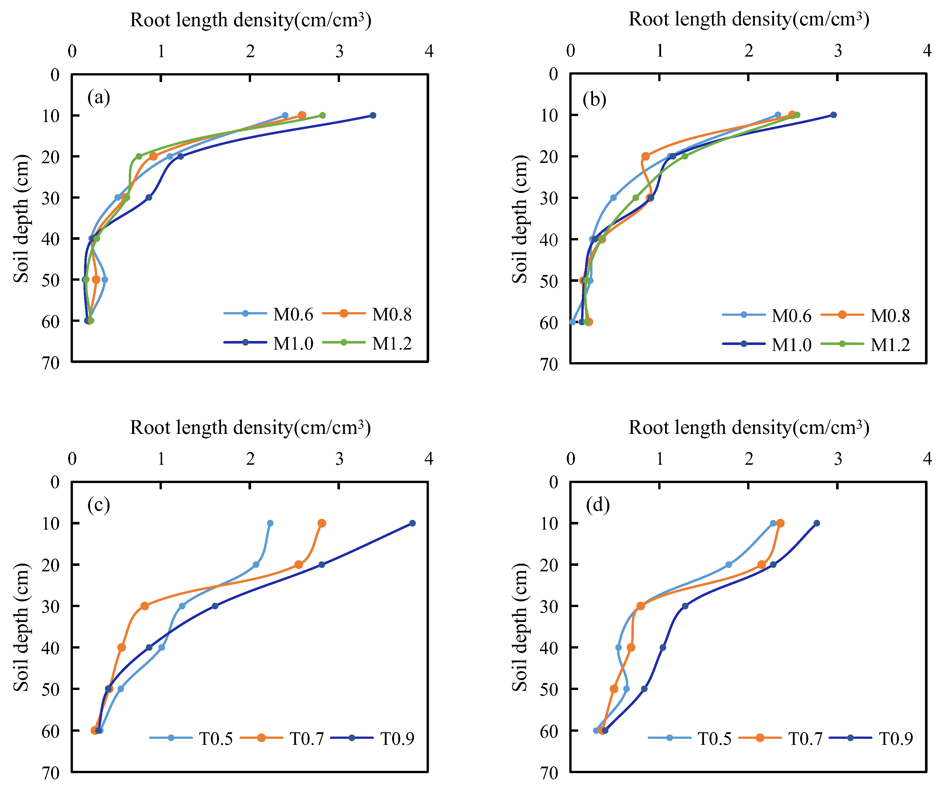
Figure 4 presents the RLD of muskmelon and tomato under varying water conditions. It can be observed that the RLD in the 0–40 cm soil layer accounted for more than 85% of the total. The RLD was the highest in the topsoil (0–10 cm) and gradually decreased with increasing soil depth. For muskmelon, the maximum RLD occurred at the 10 cm depth under the M1.0 treatment, with the maximum values of 3.38 and 2.96 cm·cm⁻³ in the two experimental years, respectively. The minimum RLD was recorded at the 60 cm depth under the M0.6 treatment, which was less than 0.2 cm·cm⁻³. For tomato, the maximum RLD also appeared at the 10 cm depth under the high-water treatment (T0.9), with maximum values of 3.83 and 2.77 cm·cm⁻³ in the two years, respectively. The minimum RLD was observed at the 60 cm depth under the T0.5 treatment, which was less than 0.3 cm·cm⁻³. A comparison of the average RLD in the 0–40 cm soil layer across different water treatments revealed that the average RLD was the highest under the M1.0 (muskmelon) and T0.9 (tomato) treatments. Specifically, the average RLD under M1.0 was 23.3%, 18.5%, and 14.3% higher than that under M0.6, M0.8, and M1.2, respectively. For tomato, the average RLD under T0.9 was 27.6% and 22.5% higher than that under T0.7 and T0.5, respectively. It is worth noting that under the severe-water-deficit treatments (M0.6 for muskmelon and T0.5 for tomato), the RLD showed a slight increasing trend at depths below 50 cm. This phenomenon may be attributed to the hydrotropic characteristics of roots induced by water stress.

3.3. Yield, Water Consumption and Water Use Efficiency

Water regulation is crucial for fruit yield, water consumption (ET), water use efficiency (WUE), and irrigation water use efficiency (IWUE), particularly for crops grown in greenhouses.

Table 4. Irrigation amount (I_r), water consumption (ET), yield, water use efficiency (WUE) and irrigation water use efficiency (IWUE) of muskmelon and tomato grown in the greenhouse under different irrigation amounts.

Year	Crops	Treatments	Ir/mm	ET/mm	Yield/(t·hm−2)	WUE/(kg·m−3)	IWUE/(kg·m−3)
2023	Muskmelon	M0.6	55.4	67.5 d	15.4 c	22.81 b	27.80 bc
		M0.8	60.8	83.1 c	19.5 bc	23.47 a	32.07 a
		M1.0	85.7	105.5 b	25.3 ab	23.98 a	29.52 b
		M1.2	110.6	124.2 a	28.5 a	22.95 ab	25.77 c
	Tomato	T0.5	177.6	256.2 c	123.3 b	48.13 a	69.43 a
		T0.7	224.4	286.4 b	128.5 b	44.87 b	57.26 b
		T0.9	286.8	322.7 a	148.6 a	46.05 ab	51.81 b
2024	Muskmelon	M0.6	51.2	65.3 c	14.6 c	22.36 ab	28.52 b
		M0.8	64.5	86.9 b	18.9 b	21.75 b	29.30 ab
		M1.0	87.8	112.2 ab	26.9 a	23.98 a	30.64 a
		M1.2	116.6	133.7 a	25.4 a	19.00 c	21.78 c
	Tomato	T0.5	175.4	172.6 c	127.6 c	73.93 a	72.75 a
		T0.7	291.2	291.2 b	132.7 b	45.57 b	45.57 b
		T09	340.6	341.3 a	158.4 a	46.41 b	46.51 b

Values with different lowercase letters (a–d) differ significantly at the 0.05 probability level.

presents the irrigation amount (I_r), ET, yield, WUE, and IWUE of muskmelon and tomato under different water treatments in 2023 and 2024. It can be observed that ET was positively proportional to I_r, with ET gradually increasing as I_r increased. ET of tomato was higher than that of muskmelon, with the maximum ET reaching 341.3 mm (T0.9), which was more than 60% higher than the maximum ET of muskmelon. The yield of muskmelon showed no significant difference between M1.0 and M1.2 but was significantly higher than that of M0.6 and M0.8. Specifically, the yield of M1.0 was 39.1–45.7% higher than that in M0.6 (Table 4). For tomato, significant differences in yield were observed among the three water treatments, except in 2023, when no significant differences were found. The yield of T0.9 was 13.5–16.2% and 17.0–19.4% higher than T0.7 and T0.5, respectively (Table 4).

With the increase in irrigation amount, WUE and IWUE of muskmelon first increased and then decreased, while tomatoes showed a gradual decreasing trend in WUE and IWUE. For muskmelon, the maximum WUE and IWUE were observed in M0.8 (2023) and M1.0 (2024), respectively, and there were no significant difference in WUE and IWUE between the two treatments. Both treatments had significantly higher WUE and IWUE than those in M0.6 and M1.2. Specifically, WUE of muskmelon in these two optimal treatments was 3.0% and 10.0% higher than that in M0.6 and M1.2, respectively, while IWUE was 7.3% and 21.8% higher (Table 4). For tomato, WUE and IWUE of T0.5 were significantly higher than those in T0.7 and T0.9. Specifically, WUE of T0.5 was 25.9% and 24.2% higher than T0.7 and T0.9, respectively, and IWUE was 27.7% and 30.8% higher, respectively (Table 4).

These results indicated that a moderate increase in irrigation amount was indeed conducive to an increase in yield for both muskmelon and tomato, but it might not necessarily result in the maximum WUE and IWUE. Therefore, it is recommended that mild deficit irrigation may be adopted in water-scarce areas to improve water use efficiency, while full irrigation may be adopted in water-abundant areas to maximize fruit yield.

3.4. Simulation of LAI, SWC and Soil CO₂ Emission Using the WHCNS-Veg Model

The WHCNS-Veg model was calibrated by using field-measured data of SWC, LAI, and soil CO₂ emissions from M1.2 (muskmelon) and T0.9 (tomato) in 2023. Subsequently, the model was validated with measured data from other treatments in 2023 and all treatments in 2024. The soil hydraulic parameters for two greenhouses were set as the measured values, while other parameters were adjusted via the trial-and-error method to ensure that the simulated values matched the measurements as closely as possible. The adjusted parameters are presented in

Table 5. Range and estimated values of the optimized WHCNS-Veg input parameters.

Groups	Parameters	Descriptions	Optimized Values
			Muskmelon	Tomato
Soil hydraulic parameters	Ks1, Ks2, Ks3, Ks4	Saturated hydraulic conductivity (cm·d−1)	25.1, 6.3, 27.5, 25.3	4.5, 4.1, 3.0, 2.8
	θs1, θs2, θs3, θs4	Saturated soil water content (cm3·cm−3)	0.355, 0.337, 0.394, 0.402	0.395, 0.391, 0.366, 0.367
	α1, α2, α3, α4	The inverse of the air-entry value	0.058, 0.059, 0.024, 0.024	0.0026, 0.0022, 0.0015, 0.0031
	n1, n2, n3, n4	Pore size distribution index	1.66, 1.382, 1.424, 1.263	1.493, 1.471, 1.423, 1.432
Crop parameters	Kini	Crop coefficient in initial stage	0.58	0.49
	Kmid	Crop coefficient in middle stage	0.82	0.81
	Kend	Crop coefficient in end stage	0.71	0.69
	Tsum	Accumulated temperature (°C)	1495	1487
	aDM	Dry matter accumulation empirical parameter (t·ha−1)	0.53 (0.36–4)	1.51 (0.36−4)
	σy	Standard deviation of the harvested parts (t·ha−1)	0.4 (0.3–0.5)	0.41 (0.3–0.5)
	Rmax	Maximum root depth (cm)	50.0	59.8
	Ncrit	The critical N concentration of plant (%)	1.98 (0.3–2.8)	2.06 (0.3–2.8)
	Nmax	The maximum N concentration of plant (%)	2.38 (0.3–5.6)	2.55 (0.3–5.6)
Organic parameters	AOM1:AOM2	Ratio of the slow storage pool to the fast storage pool of the added organic matter	23	23
	SMB1:SMB2	Ratio of the slow pool to the fast pool of microbial organic matter	1	1
	SOM1:SOM2	Ratio of the slow reservoir to the fast reservoir of soil organic matter	3	3
	AOM1 to SMB1	Ratio of the added organic matter slow pool to the microbial organic matter slow pool	0.5	0.5
	AOM1 to SMB2	Ratio of the slow storage pool of added organic matter to the fast storage pool of microbial organic matter	0.5	0.5
	SMB1 to SOM 2	Ratio of the slow storage pool of microbial organic matter to the fast storage pool of soil organic matter	0.6	0.6
	SMB2 to SOM2	Ratio of microbial organic matter fast pool to soil organic matter fast pool	0.6	0.6
	SOM2 to SOM1	Ratio of the fast pool to the slow pool of soil organic matter	0.1	0.1
	Vn	Potential nitrification rate (mg·L−1·d−1·N)	50	49
	Kn	Saturation constant (mg·L−1·N)	110	100
	Kd	Zero-order denitrification rate constant	1	1
	Ad	Denitrification experience proportion parameter (mg·mg−1)	0.1	0.15
	Kv	First-order kinetic parameters of ammonia volatilization (day−1)	0.02	0.02

.

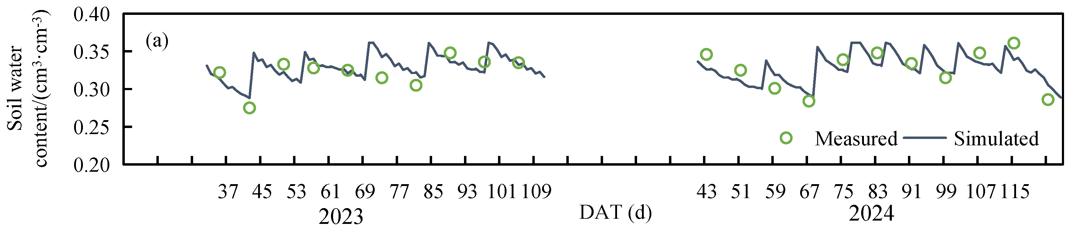
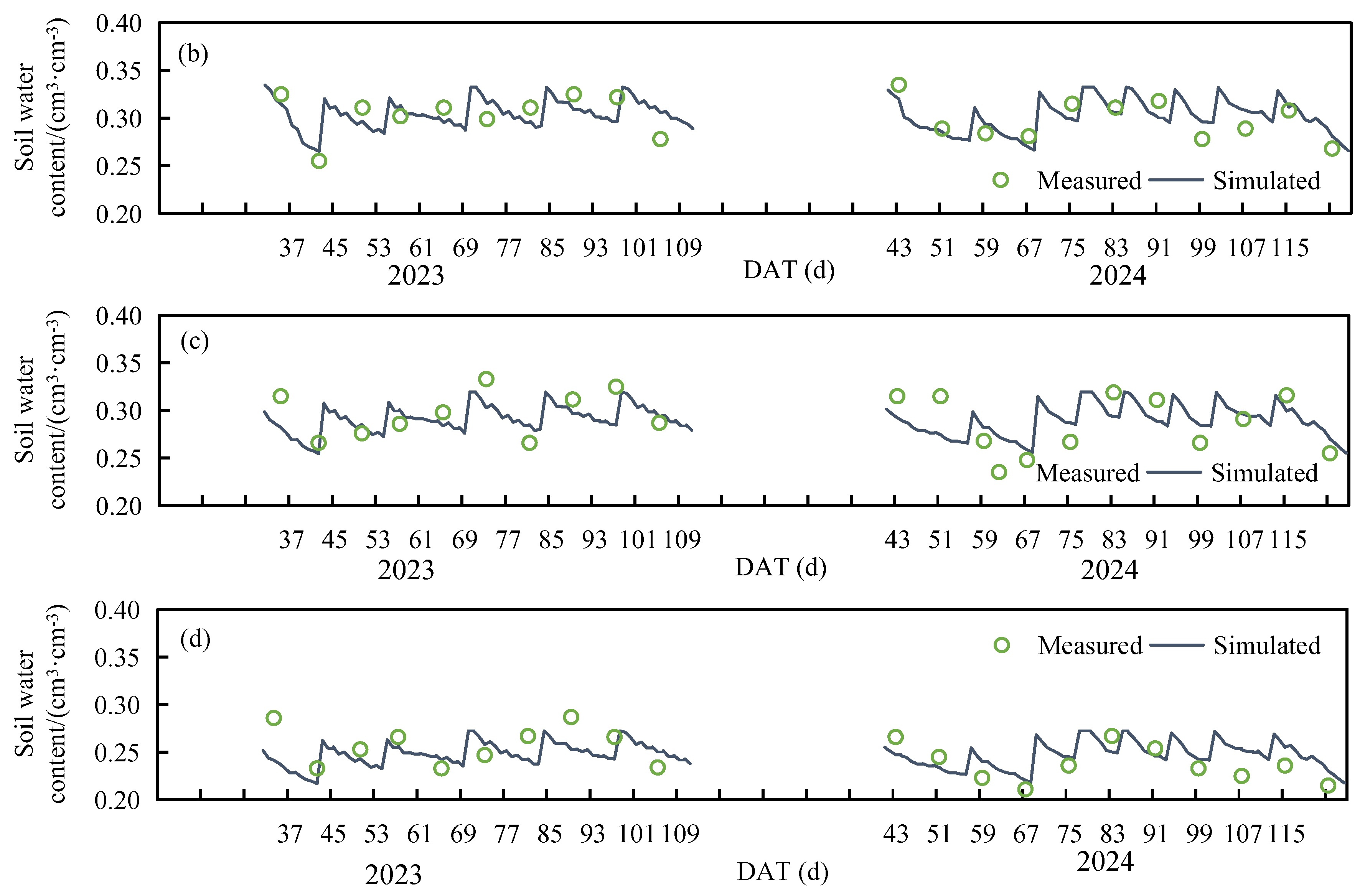
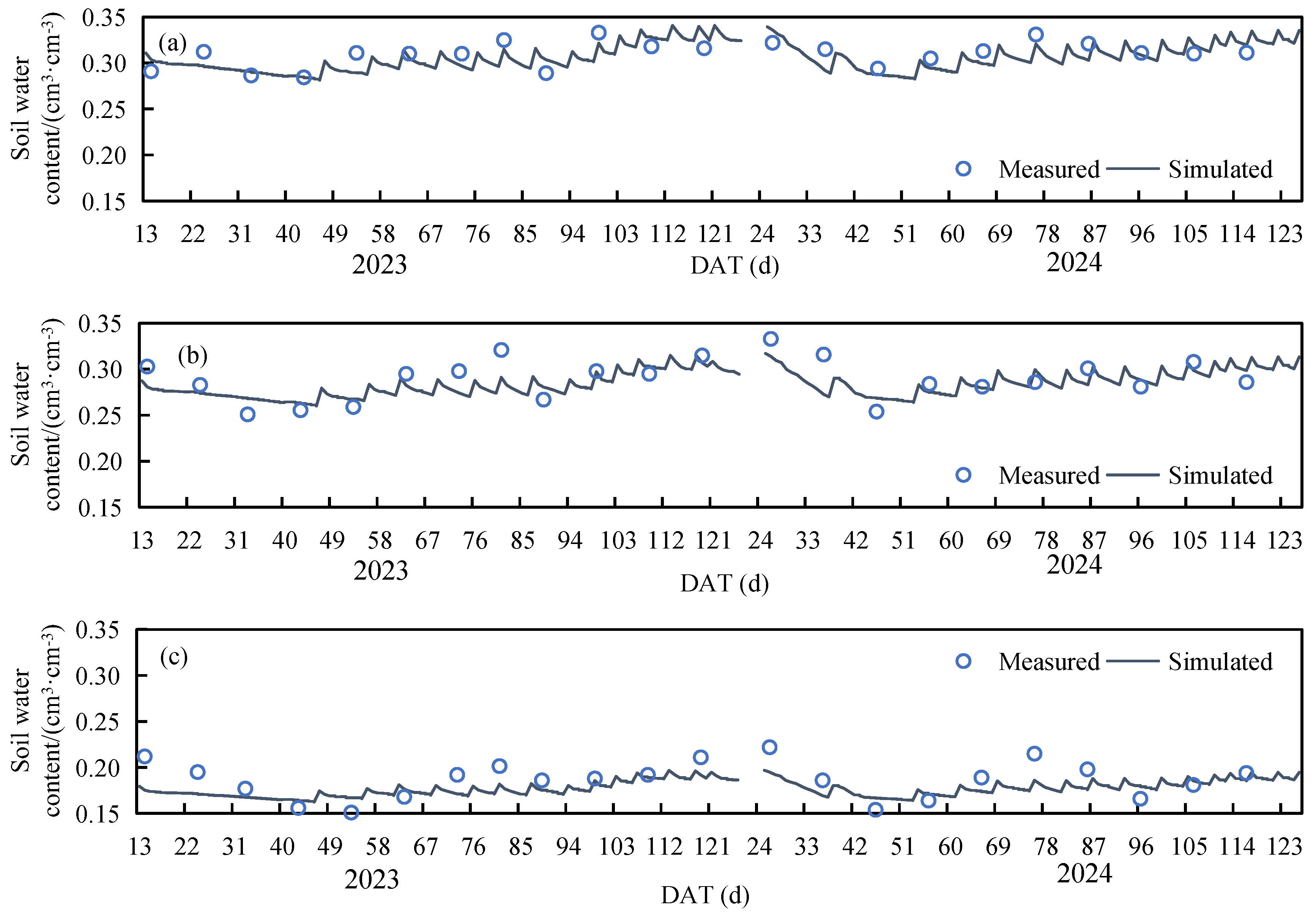
Figure 5 and Figure 6 respectively display the dynamics of measured and simulated average SWC values in the 0–60 cm soil layer for muskmelon and tomato under different water levels. We found that SWC under high-water treatments was higher than that under low-water treatments. In terms of the average value across the entire growth period, SWC of muskmelon under M1.2 was 7.4%, 11.5%, and 24.6% higher than that under M1.0, M0.8, and M0.6, respectively. For tomato, SWC under T0.9 was 7.6% and 4.3% higher than that under T0.7 and T0.5, respectively. For SWC calibration using the WHCNS-Veg model, the RMSE and EF yielded were 0.014 cm³·cm⁻³ and 0.578, respectively. During the model validation process, RMSE ranged from 0.013 to 0.022 cm³·cm⁻³, and EF varied from 0.533 to 0.789 (

Table 6. Statistical indicators comparing estimated soil water content (SWC), leaf area index (LAI), and soil CO₂ emission volume by the WHCNS-Veg model and measurements of muskmelon and tomato grown in the greenhouse in two study years. The data for the two years are the pooled data for SWC and soil CO₂ emissions.

Crops	Treatments	SWC		Soil CO2 Emission Flux		LAI
						2023		2024
		RMSE/ (cm3·cm−3)	EF	RMSE/ (kg·hm−2)	EF	RMSE/ (cm2·cm−2)	EF	RMSE/ (cm2·cm−2)	EF
Muskmelon	M1.2	0.014	0.578	1.934	0.880	0.132	0.983	0.103	0.985
	M1.0	0.015	0.533	1.057	0.916	0.131	0.989	0.125	0.988
	M0.8	0.022	0.552	1.799	0.853	0.141	0.972	0.155	0.976
	M0.6	0.017	0.607	1.910	0.863	0.146	0.971	0.155	0.975
Tomato	T0.9	0.013	0.591	1.701	0.936	0.163	0.971	0.146	0.962
	T0.7	0.017	0.545	2.188	0.804	0.147	0.964	0.147	0.96,3
	T0.5	0.018	0.789	1.860	0.893	0.210	0.888	0.152	0.944

). Overall, these indicators met the corresponding criteria (RMSE < 0.05 cm³·cm⁻³, EF > 0.5). Therefore, the WHCNS-Veg model can effectively simulate SWC of muskmelon and tomato in the 0–60 cm soil layer under varying water conditions.

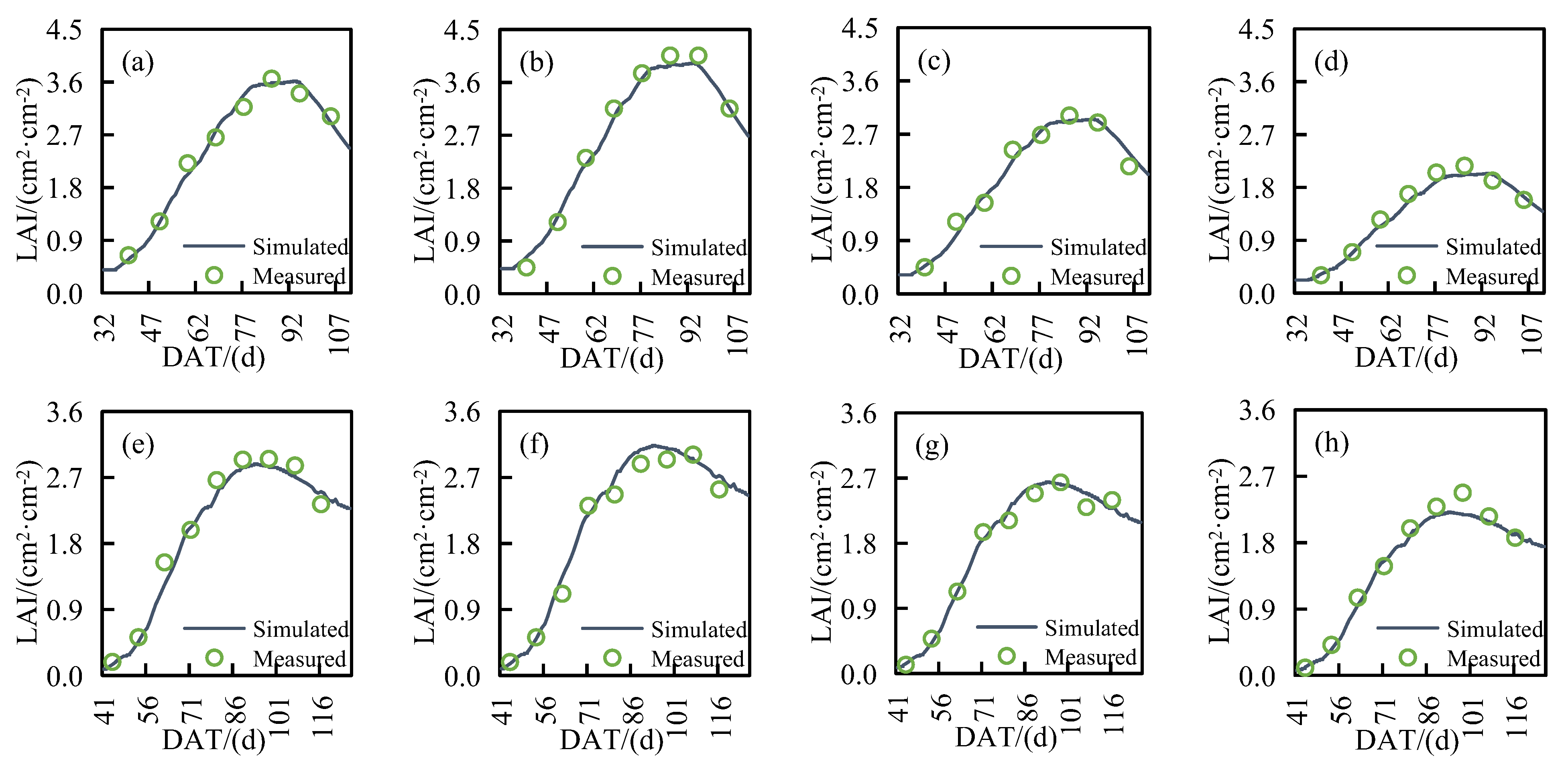
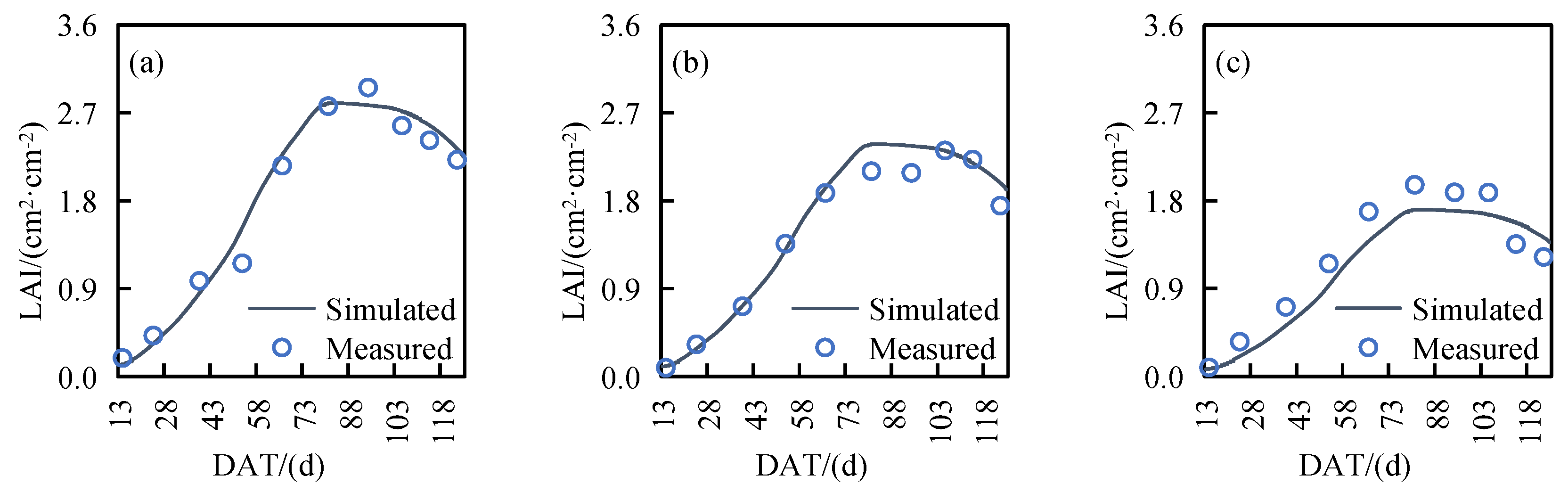
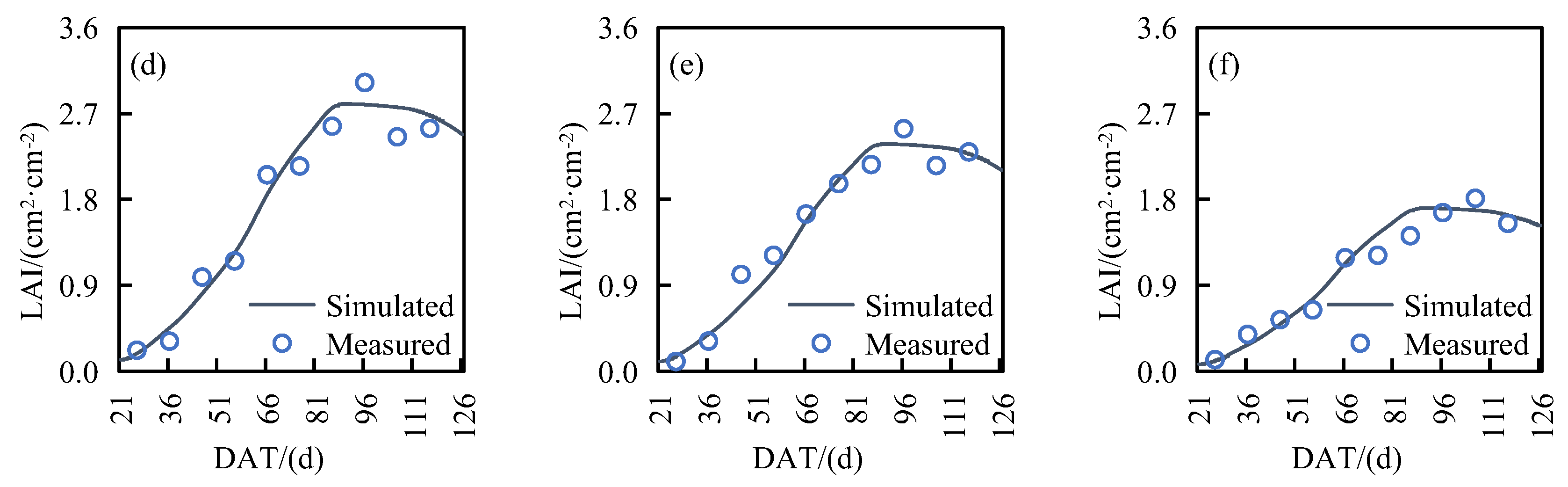
Figure 7 and Figure 8 respectively present the comparisons between measured and simulated LAI values for muskmelon and tomato under different water levels. We found that the dynamics of LAI across all treatments were similar over the two study years. Furthermore, the WHCNS-Veg model could effectively capture the LAI developmental trends of all treatments, with relatively low RMSE values (0.10 cm²·cm⁻² < RMSE < 0.21 cm²·cm⁻²) and high EF values (0.88 < EF < 0.99) (Table 6). Specifically, for muskmelon, the performance of the model simulation under high-water treatments (M1.2 and M1.0) was superior to those under low-water treatments (M0.8 and M0.6). Among the high-water levels, the accuracy in 2024 was better than that in 2023, whereas the opposite trend was observed for the low-water levels across the two years. Similarly, for tomato, the performance of the model simulation under the high-water treatment (T0.9) was superior to that under moderate deficit (T0.7) and severe deficit (T0.5) treatments, with consistent simulation results between the two years. In addition, for the severe-water-deficit treatments (M0.6 for muskmelon and T0.5 for tomato), the simulated LAI values underestimated the measurements of LAI. The main reasons for these phenomena were that those droughts shortened the plant growth cycle, thereby affecting LAI development. The WHCNS-Veg model simulated LAI based on temperature, light, and RDS parameter factors, thus being able to capture the LAI growth characteristics well.

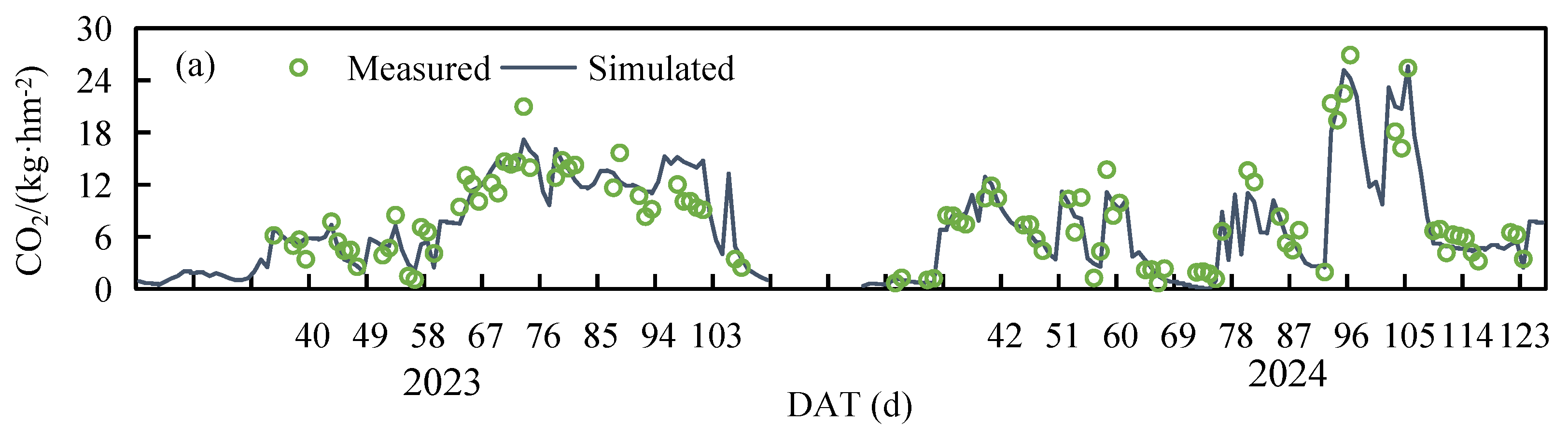
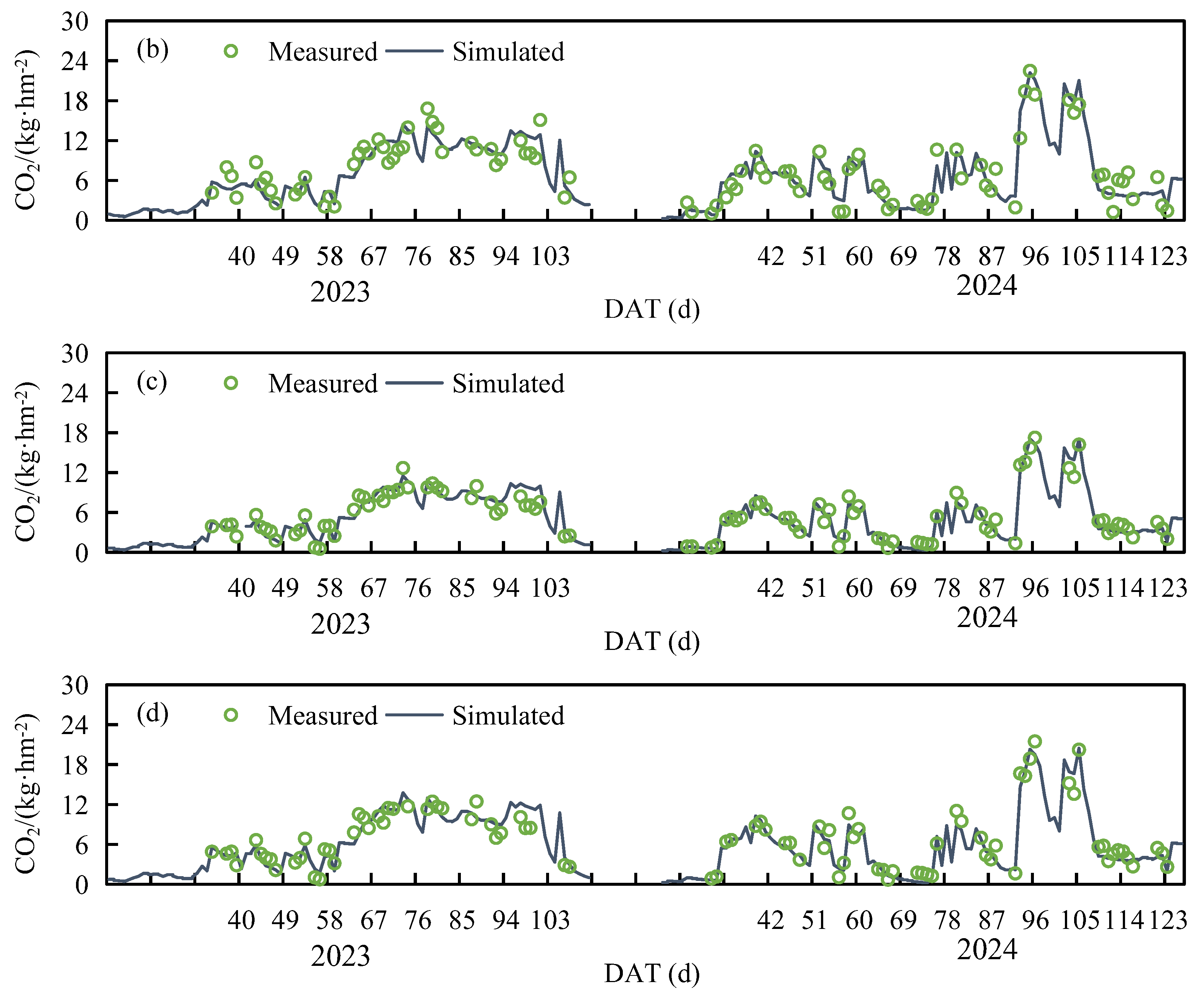
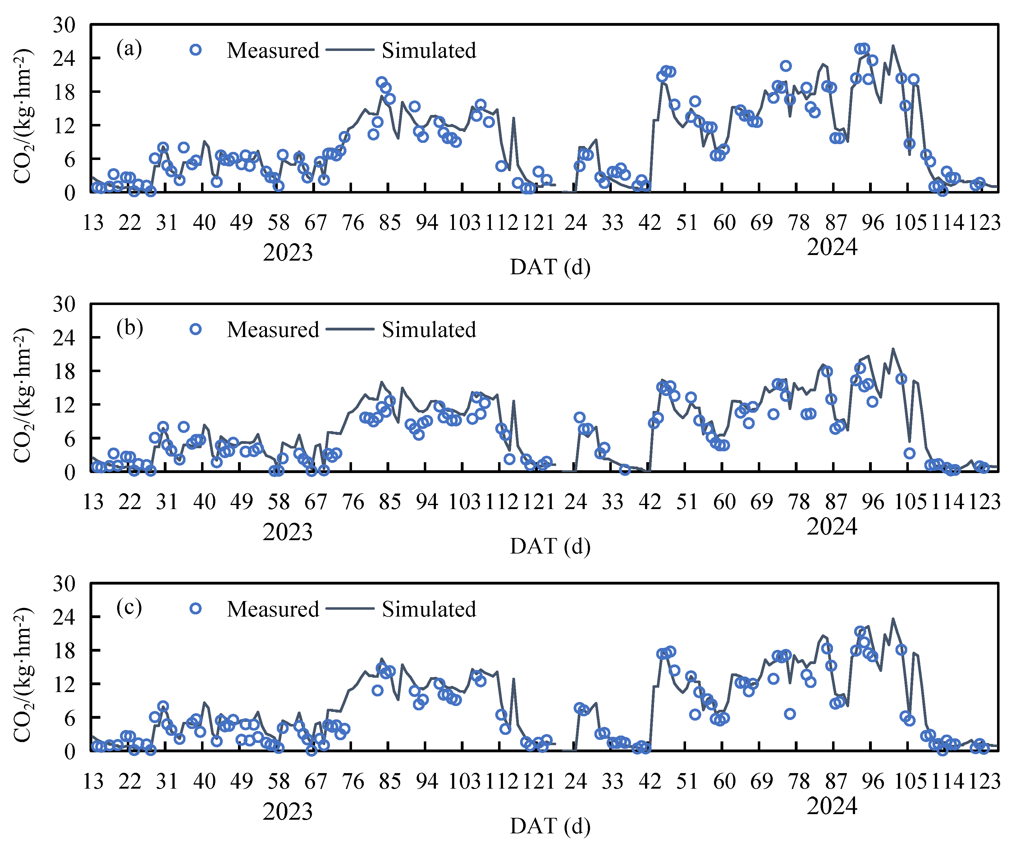
Figure 9 and Figure 10 respectively display the dynamics of measured and simulated soil CO₂ emission fluxes for muskmelon and tomato under different water levels. We found that the variations in soil CO₂ emission fluxes were relatively similar for both crops across all water treatments, showing a trend of first increasing and then decreasing during the entire growth period. Furthermore, the soil CO₂ emission fluxes under high-water treatments were higher than the low-water treatments. Specifically, the daily average soil CO₂ emission flux of muskmelon under M1.2 over the two years was 8.31 kg·hm⁻², which increased by 9.2%, 32.2%, and 17.8% compared with that under M1.0, M0.8, and M0.6, respectively. Notably, the daily average soil CO₂ emission flux under M0.8 was lower than that under M0.6. The main reason may be that M0.6 severely restricted plant growth, leading to the accumulation of organic matter and microorganisms in the root zone. Meanwhile, severe water deficit increased soil temperature, thereby accelerating soil CO₂ emissions. For tomato, the daily average soil CO₂ emission flux under T0.9 over the two years was 8.67 kg·hm⁻², which was 24.6% and 22.4% higher than that under T0.7 and T0.5, respectively. In contrast, the daily average soil CO₂ emission fluxes between the T0.7 and T0.5 were relatively similar in magnitude.

The WHCNS-Veg model effectively captured the variations in daily average soil CO₂ emission fluxes across all treatments, with RMSE ranging from 1.05 to 2.19 kg·hm⁻² and EF varying from 0.80 to 0.94 (Table 6). For muskmelon, the model exhibited the best performance under M1.0, while the performance of the model simulation was relatively poor under M0.6. For tomato, the model exhibited the optimal performance under T0.9. The main reason for these results was that the WHCNS_Veg model employs the nested Daisy model to simulate soil CO₂ emissions, and the equations involved in this model are mainly related to nitrogen mineralization and immobilization processes and soil microbial activity. Moderate water levels are conducive to nitrogen mineralization, immobilization, and soil microbial activity. However, the model does not yet consider the impact of water stress, consequently reducing its accuracy.

4. Discussion

4.1. Effects of Irrigation Levels on Crop Growth and Water Use Efficiency in Greenhouses

Our study revealed significant differences in the optimal irrigation thresholds between muskmelon and tomato grown in greenhouses. For muskmelon, the highest yield was achieved under the 1.0 and 1.2 E_p levels, and there was no significant difference observed between these two treatments over the two study years. In contrast, tomato exhibited the maximum yield under the 0.9 E_p level, which was significantly higher than that under water-stressed treatments (0.7 E_p and 0.5 E_p). This discrepancy essentially arises from the heterogeneity in physio-ecological characteristics and water requirements across growth stages of the two crops. As a shallow-rooted crop, muskmelon has roots primarily distributed in the 0–20 cm soil layer and is highly sensitive to topsoil moisture [15]. A moderately sufficient water supply (1.0 E_p or 1.2 E_p) can ensure root elongation and nutrient uptake, facilitate photosynthate translocation to fruits, and thereby enhance yield. However, no significant yield increase was detected when the irrigation amount exceeded 1.0 E_p. This may be attributed to excessive water reducing soil porosity and inducing root hypoxia, which inhibits root respiration and nutrient uptake and transport and instead triggers excessive vegetative growth and nutrient competition with reproductive growth [42]. Compared with muskmelon, tomato possesses relatively well-developed deep roots and exhibits slightly stronger drought resistance. A moderate water supply of 0.9 E_p can regulate stomatal conductance and photosynthetic rate, optimize source–sink relationships, and promote dry matter accumulation during the fruit expansion stage. In contrast, water stress below 0.7 E_p leads to premature leaf senescence, reduced photosynthetic area, and suppressed pollen viability and fruit set rate, ultimately resulting in a significant yield reduction [43]. The inhibitory effect of water stress on crop reproductive growth is more pronounced in muskmelon. Our study found that when the irrigation amount was below 0.8 E_p, muskmelon RLD was significantly reduced. This is consistent with previous research conclusions that crops prioritize vegetative growth while inhibiting reproductive growth under water stress [7]. Previous studies have also found that water deficiency increased the content of abscisic acid (ABA) in plants, which, in turn, inhibited the synthesis of gibberellic acid and indole-3-acetic acid, leading to a reduced fruit set rate and increased fruit malformation rate [44]. In contrast, under mild water stress, tomato can reduce transpiration water loss by closing some stomata while maintaining a relatively high photosynthetic rate, thereby achieving a balance between WUE and yield [18].

The trade-off between maximizing yield and optimizing WUE is one of the core contradictions in water-saving irrigation research. Our study found that for muskmelon, the treatments with the highest yield (1.0 E_p) had a significantly lower WUE than that under 0.6 E_p. Similarly, the WUE of the optimal yield treatment (0.9 E_p) was also lower than that under 0.5 E_p for tomato. This result is consistent with the conclusions of most studies on greenhouse crop irrigation [6,7,16,45,46], indicating that sufficient water can ensure yield but reduces WUE due to increased transpiration consumption. Our study further clarified the balance thresholds between yield and WUE for greenhouse crops. The optimal balance threshold for muskmelon was 1.0 E_p, at which the yield decreased by approximately 2.7% compared with that under 1.2 E_p, but WUE and IWUE increased by 12.5% and 20.8%, respectively. For tomato, the balance threshold was 0.9 E_p, which ensures the maximum yield while also preventing a significant decline in WUE and IWUE. The determination of these balance thresholds provides key parameters for achieving the synergistic goals of water conservation and yield increase in greenhouse crops. In-depth analysis revealed that muskmelon experienced heat stress and strong radiation during the late growth stage in 2023. To mitigate the damage to plants caused by heat stress, a 5 mm mist cooling treatment was applied to the M0.8 treatment. This practice did not induce instability in the internal greenhouse microclimate, and all experimental data of the M0.8 treatment in this study were analyzed under this measure, with the corresponding water volume fully incorporated into the total irrigation amount. The 5 mm mist cooling only alleviated the high-temperature stress inside the greenhouse and did not interfere with the normal water demand of crops [1,11]. The conclusions of our study regarding the optimal irrigation thresholds for crops differ somewhat from those of some previous studies. For example, Gao et al. [46] reported that the maximum yield of autumn muskmelon was achieved at SWC lower and upper limits of 65% θ_f to 100% θ_f, which is slightly different from the optimal irrigation levels (1.0 E_p, corresponding to SWC of 75% θ_f to 90% θ_f). This discrepancy is mainly attributed to differences in light, T_a, and moisture conditions caused by varying growth seasons. Excessively high SWC (exceeding 90% θ_f) is prone to causing root hypoxia, which, in turn, inhibits growth [17]. Mahajan et al. [47]. indicated that tomatoes grown in greenhouses under drip irrigation could achieve the maximum yield at 0.5 E_p, but this required the application of 100% recommended nitrogen fertilizer. This conclusion differs significantly from our study, where the optimal yield of tomato was at 0.9 E_p. The key factor contributing to this difference is the water–nitrogen coupling effect. High nitrogen supply alleviated the inhibitory effect of severe water stress on tomato growth, whereas, in our study, a uniform recommended nitrogen application rate was adopted, and under severe water stress (0.5 E_p), nitrogen uptake was hindered, leading to restricted plant growth [44]. In addition, Li et al. [43] found that 0.8 E_p was conducive to increasing the yield of greenhouse tomatoes under alternate furrow irrigation conditions, which is consistent with the balance threshold identified in our study. Nevertheless, the absolute value of the optimal irrigation amount differs due to the variation in irrigation methods. In addition, differences in regional climate and soil texture also affect crop water requirement thresholds. Li et al. [15] suggested that the water deficit threshold for muskmelon is approximately 55% θ_f, and below this threshold, yield, WUE, and IWUE all decrease significantly. This threshold differs from that identified in our study. The main reason is that the above study was conducted in a semi-arid region with sandy loam soil, which has a poor water retention capacity.

4.2. Effects of Irrigation Levels on Soil CO₂ Emissions in Greenhouses

In our study, in situ observations revealed that the daily average soil CO₂ emission fluxes of muskmelon and tomato ranged from 5.63 to 8.67 kg·hm⁻², which falls within the range of the soil CO₂ emissions from protected vegetable fields reported in previous studies [28,48,49,50] but is significantly higher than those from field crops (e.g., maize and wheat) [51,52]. Compared with open-field cultivation, T_a and RH in closed greenhouse environments are significantly higher than those in field conditions, providing suitable environmental conditions for soil microbial activity. Meanwhile, mature organic fertilizers are commonly applied in protected vegetable cultivation, resulting in high organic carbon input that serves as sufficient substrates for microbial respiration, thereby significantly promoting heterotrophic respiration processes [48,49,51,53]. A study by Lin et al. [51] reported that the average soil CO₂ emission flux of greenhouse vegetable fields with three years of cultivation history was 1.39 times that of maize fields, which is consistent with the results of our study. Irrigation level is a key regulatory factor governing soil CO₂ emissions in greenhouses. Our study found that soil CO₂ emission fluxes significantly increased with increasing SWC, a finding consistent with the conclusion of Zeng et al. [54] that the soil respiration rate of greenhouse tomato is significantly positively correlated with SWC. Regulation of soil CO₂ emissions by water is primarily achieved through the following pathways. Firstly, water serves as an essential condition for microbial metabolism, and low SWC leads to a decrease in microbial activity and weakened metabolism, thereby inhibiting heterotrophic respiration. Secondly, SWC affects the diffusion rate of CO₂ in soil pores, and moderate moisture promotes the diffusion of CO₂ from the soil interior to the atmosphere; in contrast, insufficient moisture results in soil pores being filled with air, increasing CO₂ diffusion resistance and reducing emission fluxes. Thirdly, water indirectly regulates root respiration by influencing crop root growth, and sufficient moisture promotes root development, increases root biomass and respiration rate, and consequently enhances total soil respiration flux. Nevertheless, some studies have reported contrasting conclusions. Lin et al. [51] found that the relationship between soil CO₂ emission flux and SWC in greenhouse vegetable fields follows a logarithmic or parabolic pattern, whereas Chen et al. [28] argued that there is a negative correlation between soil CO₂ emission flux and SWC in greenhouse tomato fields. This discrepancy is primarily due to variations in the range of SWC investigated. When SWC is between 60% θ_f and 80% θ_f, the regulatory effect of water on soil respiration is not significant [54]. In our study, SWC under all irrigation treatments mainly ranged from 60% θ_f to 90% θ_f; thus, an overall trend of increasing emission fluxes with increasing moisture was observed. However, the rate of increase in emission flux under the 1.2 E_p treatment slowed down significantly, indicating that oxygen deficiency had begun to act as a limiting factor at this water level.

Soil CO₂ emission fluxes for the two crops exhibited a trend of first increasing, then decreasing, and finally stabilizing at a relatively high level throughout the entire growth period, with peak values both occurring during the flowering–fruiting stage. This dynamic characteristic is highly coupled with the crop growth process, and its core driving factor is the synergistic changes between root respiration and heterotrophic respiration [51]. From transplantation to the flowering–fruiting stage, crop root biomass continuously increased, root activity was significantly enhanced, and root respiration rate gradually rose, becoming one of the main sources of soil CO₂ emissions. After entering the fruit ripening stage, soil CO₂ emission flux showed a decreasing trend but remained at a relatively high level [51]. At this stage, crop root growth slowed or even degenerated, and root respiration rate decreased, which became the main reason for the decline in emission flux. However, the soil microbial biomass was still at a high level, and the increased decomposition of plant residues (e.g., senescent leaves and roots) during fruit ripening provided sufficient substrates for microorganisms, maintaining a stable heterotrophic respiration rate [22]. Thus, soil CO₂ emission flux did not decrease significantly. This result is consistent with the research conclusions of Sainju et al. [55]; thereby, the temporal dynamics of soil CO₂ emissions during the crop growth period are essentially the result of the trade-off between root respiration and heterotrophic respiration.

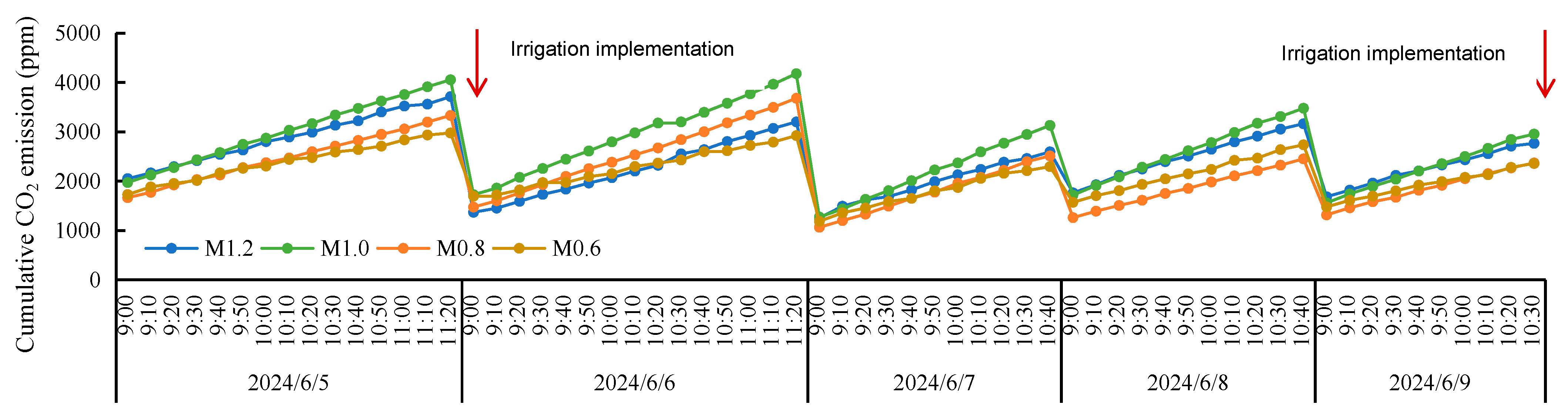
When the soil is under water-deficit conditions, soil microorganisms are rapidly reactivated after rehydration under drip irrigation, with a significant enhancement in their metabolic activity. This leads to the decomposition of soil organic matter and subsequent massive release of CO₂, thus inducing a significant short-term surge in soil CO₂ emission fluxes. For this reason, we focused on analyzing the ‘Birch effect’ under different water regimes in the context of drip irrigation and elaborated on this effect by taking the experimental data of greenhouse muskmelon as a case study. Figure 11 shows that the ‘Birch effect’ was observed in the deficit irrigation regimes for greenhouse muskmelon after irrigation in 2024. During a complete irrigation event, the cumulative CO₂ emissions in the M0.8 treatment increased after irrigation on June 6 and exceeded those in the M1.2 regime after 10:30. Similarly, measurements conducted on June 7 showed that the M0.6 and M0.8 treatments had relatively higher CO₂ emissions, with no significant difference from those in the M1.2 regime. However, the CO₂ emissions in the water-deficit M0.6 and M0.8 treatments declined after June 8. This ‘Birch effect’ fully illustrates that under drip irrigation conditions, the metabolic rate of the microbial community rebounded rapidly in a short period after localized soil rehydration, which acted as the biological basis for CO₂ release. Meanwhile, the pores between soil particles were moderately filled with water, which optimized soil aeration, further enhanced the respiratory activity of microorganisms, and thereby accelerated the production.

4.3. Performance of the WHCNS-Veg Model in Greenhouse

Based on the soil module of the WHCNS model, our study constructed a process-based model for water–carbon management in protected vegetable fields (WHCNS-Veg) by incorporating the vegetable growth simulation approach from the EU-Rotate_N model and improving the original crop growth module. The model was successfully applied to simulate SWC, LAI, and soil CO₂ emission fluxes for muskmelon and tomato grown in greenhouses. The results indicated that the WHCNS-Veg model exhibited high accuracy in greenhouse environments. For SWC, the RMSE ranged from 0.013 to 0.022 cm³·cm⁻³ and the EF from 0.533 to 0.789. For LAI, the RMSE varied between 0.103 and 0.210 cm²·cm⁻² and the EF between 0.888 and 0.989. For soil CO₂ emission fluxes, the RMSE was changed from 1.057 to 2.188 kg·hm⁻² and the EF from 0.804 to 0.936. Among these, the accuracy of LAI and CO₂ emission fluxes was relatively higher, indicating that the model can accurately simulate the coupled processes of crop growth and soil respiration. In contrast, the performance of the model in simulating SWC was relatively lower, which may be attributed to the following factors. Firstly, the model does not fully consider the spatial heterogeneity of SWC under drip irrigation. Secondly, the soil hydraulic parameters in the model are derived from laboratory experiments, which differ from the actual field soil conditions, resulting in simulation errors in soil water infiltration and evaporation processes.

Our study further verified the applicability of the WHCNS-Veg model in simulating soil CO₂ emissions in greenhouse environments. After calibrating the WHCNS-Veg model, Liang et al. [53] reported that it performed well in simulating the water–heat–carbon–nitrogen transport processes of greenhouse vegetables, with the normalized root mean square error of SWC, yield, and vegetable nitrogen uptake reduced to 5.7%, 2.7%, and 8.3%, respectively. Furthermore, Li et al. [56] evaluated the model’s performance in simulating N₂O and NH₃ emissions under different irrigation levels for greenhouse cucumber and tomato and found that the accuracy of N₂O and NH₃ emissions ranged from 0.011~0.037 kg·hm⁻² and 0.12~0.46 kg·hm⁻², respectively. The results of soil CO₂ emission fluxes in our study complement the data gap of the WHCNS-Veg model in greenhouse carbon cycle simulation, confirming that the model can effectively capture the dynamic changes in soil CO₂ emissions driven by irrigation levels. However, the model exhibited relatively larger simulation errors during the peak CO₂ emission period (RMSE up to 2.188 kg·hm⁻²). The main reason is that the calculation of root respiration in the model only considers root biomass and does not incorporate dynamic changes in root activity, while the sharp increase in root activity during the flowering and fruiting stage leads to higher actual respiration rates than the simulated values.

The construction and validation of the WHCNS-Veg model provide an effective tool for the water–carbon synergistic management for greenhouse crops. Nevertheless, studies on simulating soil CO₂ emission fluxes using the WHCNS-Veg model are still limited. Further practical validation under more greenhouse crops and different cultivation conditions is required to enhance the generality and stability of the WHCNS-Veg model.

5. Conclusions

Our study investigated the effects of different irrigation levels on muskmelon and tomato growth, RLD, yield, WUE, as well as soil CO₂ emissions while verifying the performance of the WHCNS-Veg model. The main conclusions are as follows: (1) Irrigation levels significantly regulate crop growth and yield, and the optimal yield of muskmelon was achieved at an irrigation level of 1.0 E_p, and that of tomato was achieved at 0.9 E_p. Moderate water deficit (0.8 E_p for muskmelon and 0.7 E_p for tomato) could significantly improve WUE and IWUE. (2) Soil CO₂ emission fluxes showed a trend of first increasing and then decreasing throughout the growth period. Overall, soil CO₂ emission fluxes were higher under high-water treatments. Under severe water stress, however, soil CO₂ emission fluxes increased slightly due to accelerated organic matter decomposition caused by elevated soil temperature. (3) The WHCNS-Veg model could accurately simulate SWC, LAI, and soil CO₂ emissions, with accuracy meeting research requirements. It could be applied to the simulation of water–carbon synergistic regulation for greenhouse crops.

References

1. Shamshiri, R.R.; Jones, J.W.; Thorp, K.R.; Ahmad, D.; Man, H.C.; Taheri, S. Review of optimum temperature, humidity, and vapour pressure deficit for microclimate evaluation and control in greenhouse cultivation of tomato: A review. Int. Agrophys. 2018, 32, 287–302. [Google Scholar] [CrossRef]
2. Zhao, Y.; Mao, X.M.; Shukla, M.K.; Tian, F.; Hou, M.J.; Zhang, T.; Li, S.E. How does film mulching modify available energy, evapotranspiration, and crop coeffcient during the seed–maize growing season in northwest China? Agric. Water Manag. 2021, 245, 106666. [Google Scholar] [CrossRef]
3. Sänger, A.; Geisseler, D.; Ludwig, B. Effects of rainfall pattern on carbon and nitrogen dynamics in soil amended with biogas slurry and composted cattle manure. J. Plant Nutr. Soil Sci. 2010, 173, 692–698. [Google Scholar] [CrossRef]
4. Ouma, G. Effect of different container sizes and irrigation frequency on the morphological and physiological characteristics of mango (Mangifera indica) rootstock seedlings. Int. J. Bot. 2007, 3, 260–268. [Google Scholar] [CrossRef]
5. Gong, X.; Li, X.; Qiu, R.; Bo, G.; Ping, Y.; Xin, Q.; Ge, J. Ventilation and irrigation management strategy for tomato cultivated in greenhouses. Agric. Water Manag. 2022, 273, 107908. [Google Scholar] [CrossRef]
6. Zhao, W.; Ma, F.; Cao, W.; Ma, F.; Han, L. Effects of water-fertilizer coupling on the yield and quality of tomato grown in substrate culture. Trans. Chin. Soc. Agric. Eng. 2022, 38, 95–101. [Google Scholar] [CrossRef]
7. Hu, J.; Gettel, G.; Fan, Z.; Lv, H.; Lin, S.; Zhao, Y.; Yu, Y.; Wang, J.; Butterbach-Bahl, K.; Li, G.; et al. Drip fertigation promotes water and nitrogen use efficiency and yield stability through improved root growth for tomatoes in plastic greenhouse production. Agric. Ecosyst. Environ. 2021, 313, 107379. [Google Scholar] [CrossRef]
8. Fang, Z.; Ma, F.; Cui, J.; Zheng, Z.; Feng, S.; Wang, J. Study on the root distribution pattern of processing tomato under mulched drip irrigation. Xinjiang Agric. Sci. 2008, 45, 15–20. [Google Scholar]
9. Guo, S.R. Effects of dissolved oxygen concentration in nutrient solution on respiratory intensity of cucumber and tomato roots. Acta Hortic. Sin. 2000, 27, 141–142. [Google Scholar] [CrossRef]
10. Xue, L.; Zhang, Y.; Duan, J.; Liu, N.; Wang, Z. Relationship between root distribution and water consumption of winter wheat under regulated deficit irrigation. J. Triticeae Crops 2010, 30, 693–697. [Google Scholar] [CrossRef]
11. Incrocci, L.; Thompson, R.B.; Fernandez-Fernandez, M.D.; Pascale, S.D.; Pardossi, A.; Stanghellini, C.; Rouphael, Y.; Gallardo, M. Irrigation management of european greenhouse vegetable crops. Agric. Water Manag. 2020, 242, 106393. [Google Scholar] [CrossRef]
12. Bambach, N.E.; Gilbert, M.E.; Paw U, K.T. Introducing a dynamic photosynthetic model of photoinhibition, heat, and water stress in the next-generation land surface model ACASA. Agric. For. Meteorol. 2022, 312, 108702. [Google Scholar] [CrossRef]
13. Yang, F.H.; Wu, P.T.; Zhang, L.; Wei, Y.Q.; Tong, X.Y.; Wang, Z.G. Effects of subsurface irrigation types on root distribution, leaf photosynthetic characteristics, and yield of greenhouse tomato. Sci. Hort. 2024, 112883. [Google Scholar] [CrossRef]
14. Korner, O.; Fanourakis, D.; Hwang, M.C.; Hyldgaard, B.; Tsaniklidis, G.; Nikoloudakis, N.; Larsen, D.H.; Ottosen, C.; Rosenqvist, E. Incorporating cultivar-specific stomatal traits into stomatal conductance models improves the estimation of evapotranspiration enhancing greenhouse climate management. Biosyst. Eng. 2021, 208, 131–151. [Google Scholar] [CrossRef]
15. Li, Y.J.; Yuan, B.Z.; Bie, Z.L.; Kang, Y.H. Effects of drip irrigation threshold on yield and quality of muskmelon in plastic greenhouse. Trans. Chin. Soc. Agric. Eng. 2012, 28, 132–138. [Google Scholar] [CrossRef]
16. Wu, H.M.; Yan, H.F.; Zhang, C.; Huang, S.; Joe, S.A. Responses of yield and water use efficiency of drip-irrigated greenhouse cucumber to water stress. Trans. Chin. Soc. Agric. Eng. 2020, 36, 84–93. [Google Scholar] [CrossRef]
17. Yang, H.; Du, T.S.; Qiu, R.J.; Chen, J.L.; Wang, F.; Li, Y.; Wang, C.X.; Gao, L.H.; Kang, S.Z. Improved water use efficiency and fruit quality of greenhouse crops under regulated deficit irrigation in northwest China. Agric. Water Manag. 2017, 179, 193–204. [Google Scholar] [CrossRef]
18. Hooshmand, M.; Albaji, M.; Nasab, S.B.; Ansari, N.A.Z. The effect of deficit irrigation on yield and yield components of greenhouse tomato (Solanum lycopersicum) in hydroponic culture in Ahvaz region, Iran. Sci. Hortic. 2019, 254, 84–90. [Google Scholar] [CrossRef]
19. Melillo, J.M.; Steudler, P.A.; Aber, J.D.; Newkirk, K.; Morrisseau, S. Soil warming and carbon-cycle feedbacks to the climate system. Science 2003, 298, 2173–2176. [Google Scholar] [CrossRef]
20. Davidson, E.A.; Belk, E.; Boone, R.D. Soil water content and temperature as independent or confounded factors controlling soil respiration in a temperate mixed hardwood forest. Glob. Change Biol. 2010, 4, 217–227. [Google Scholar] [CrossRef]
21. Norton, U.; Mosier, A.R.; Morgan, J.A.; Derner, J.D.; Ingram, L.J.; Stahl, P.D. Moisture pulses, trace gas emissions and soil C and N in cheatgrass and native grass-dominated sagebrush-steppe in Wyoming, USA. Soil Biol. Biochem. 2008, 40, 1421–1431. [Google Scholar] [CrossRef]
22. Flanagan, L.B.; Johnson, B.G. Interacting effects of temperature, soil moisture and plant biomass production on ecosystem respiration in a northern temperate grassland. Agric. For. Meteorol. 2005, 130, 237–253. [Google Scholar] [CrossRef]
23. Liu, X.Z.; Wan, S.Q.; Su, B.; Hui, D.F.; Luo, Y.Q. Response of soil CO2 efflux to water manipulation in a tall grass prairie ecosystem. Plant Soil 2002, 240, 213–223. [Google Scholar]
24. Wang, J.L.; Zhao, F.H.; Ouyang, Z. Effects of irrigation amount on soil respiration in wheat fields during the grain-filling stage. Acta Agric. Boreali-Sin. 2010, 25, 186–189. [Google Scholar] [CrossRef]
25. Muhr, J.; Franke, J.; Borken, W. Drying-rewetting events reduce C and N losses from a Norway spruce forest floor. Soil Biol. Biochem. 2010, 42, 1303–1312. [Google Scholar]
26. Jabro, J.D.; Sainju, U.; Stevens, W.B.; Evans, R.G. Carbon dioxide flux as affected by tillage and irrigation in soil converted from perennial forages to annual crops. J. Environ. Manag. 2008, 88, 1478–1484. [Google Scholar] [CrossRef]
27. Morugάn-Coronado, A.; García-Orenes, F.; Mataix-Solera, J.; Arcenegui, V.; Mataix-Beneyto, J. Short-term effects of treated wastewater irrigation on mediterranean calcareous soil. Soil Tillage Res. 2011, 112, 18–26. [Google Scholar] [CrossRef]
28. Chen, H.H.; Hui, J.; Cai, H.J.; Zhu, Y.; Wang, C. Regulation effects of aerated irrigation on soil CO2 emissions in tomato fields. Sci. Agric. Sin. 2016, 49, 3379–3389. [Google Scholar] [CrossRef]
29. Rahn, C.R.; Zhang, K.; Lillywhite, R.; Ramos, C.; Doltra, J.; de Paz, J.M.; Riley, H.; Fink, M.; Nendel, C.; Thorup-Kristensen, K.; et al. EU-ROTATE_N-a decision support system-to predict environmental and economic consequences of the management of nitrogen fertiliser in crop rotations. Eur. J. Hortic. Sci. 2010, 75, 20–32. [Google Scholar]
30. Nendel, C. Evaluation of best management practices for N fertilisation in regional field vegetable production with a small-scale simulation model. Eur. J. Agron. 2009, 30, 110–118. [Google Scholar] [CrossRef]
31. Liang, H.; Hu, K.L.; Sun, Y.; Lv, H.F.; Lin, S. WHCNS_Veg water and nitrogen management model for protected vegetable fields. Trans. Chin. Soc. Agric. Eng. 2020, 36, 96–105. [Google Scholar] [CrossRef]
32. Liang, H.; Hu, K.L.; Li, B.G.; Liu, H.T. Construction of a coupled model for water, heat, carbon and nitrogen processes in the soil-crop-atmosphere system. Trans. Chin. Soc. Agric. Eng. 2014, 30, 54–66. [Google Scholar] [CrossRef]
33. Sun, Y.; Hu, K.; Fan, Z.; Wei, Y.; Lin, S.; Wang, J. Simulating the fate of nitrogen and optimizing water and nitrogen management of greenhouse tomato in North China using the EU-ROTATE_N model. Agric. Water Manag. 2013, 128, 72–84. [Google Scholar] [CrossRef]
34. Sun, Y.; Hu, K.; Zhang, K.; Jiang, L.; Xu, Y. Simulation of nitrogen fate for greenhouse cucumber grown under different water and fertilizer management using the EU-ROTATE_N model. Agric. Water Manag. 2012, 112, 21–32. [Google Scholar] [CrossRef]
35. Guo, R.; Nendel, C.; Rahn, C.; Jiang, C.; Chen, Q. Tracking nitrogen losses in a greenhouse crop rotation experiment in North China using the EU-ROTATE_N simulation model. Environ. Pollut. 2010, 158, 2218–2229. [Google Scholar] [CrossRef] [PubMed]
36. Sabbagh, G.J.; Geleta, S.; Elliott, R.L.; Williams, J.R.; Griggs, R.H. Modification of epic to simulate pesticide activities: EPIC-PST. Trans. ASAE 1991, 34, 1683–1692. [Google Scholar] [CrossRef]
37. Green, W.H.; Ampt, G.A. Studies on soil physics, 1. The flow of air and water through soils. J. Agric. Sci. 1911, 4, 1–24. [Google Scholar] [CrossRef]
38. Allen, R.G.; Pereira, L.S.; Raes, D.; Smith, M. Crop Evapotranspiration: Guidelines for Computing Crop Water Requirements—FAO Irrigation and Drainage Paper No. 56; FAO: Rome, Italy, 1998.
39. Jones, C.A.; Kiniry, J.R. Ceres-Maize: A Simulation Model of Maize Growth and Development; Texas A & M University Press: College Station, TX, USA, 1987. [Google Scholar]
40. Driessen, P.M.; Konjin, N.T. Land Use System Analysis; Wageningen Agricultural University: Wageningen, The Netherlands, 1992. [Google Scholar]
41. Hansen, S.; Jensen, H.; Nielsen, N.E.; Svendsen, H. NPo-Research, A10: Daisy: Soil Plant Atmosphere System Model; The National Agency for Environmental Protection: Copenhagen, Danmark, 1990.
42. Gong, X.W.; Sun, J.S.; Liu, H.; Zhang, Y.Y.; Zhang, H.; Li, Y.; Zhou, X.F.; Lian, M.M.; Cui, J.X. Effects of different lower water limits on yield and quality of drip-irrigated greenhouse muskmelon during flowering and fruiting stages. J. Irrig. Drain. Eng. 2015, 34, 28–32. [Google Scholar] [CrossRef]
43. Li, H.Z.; Cao, H.X.; Guo, L.J.; Wu, X.Y. Effects of furrow irrigation methods and irrigation rates on comprehensive quality and yield of greenhouse tomatoes. Sci. Agric. Sin. 2016, 49, 4179–4191. [Google Scholar] [CrossRef]
44. Li, H.H.; Liu, H.; Gong, X.W.; Li, S.; Pang, J.; Chen, Z.F.; Sun, J.S. Optimizing irrigation and nitrogen management strategy to trade off yield, crop water productivity, nitrogen use efficiency and fruit quality of greenhouse grown tomato. Agric. Water Manag. 2021, 245, 106570. [Google Scholar] [CrossRef]
45. Chen, F.; Cui, N.B.; Jiang, S.Z.; Zhang, W.J.; Li, H.P.; Li, X.M.; Lv, M.; Liu, C.W.; Qiu, R.J.; Wang, Z.H. Effects of deficit drip irrigation at different growth stages on citrus leaf physiology, fruit growth, yield, and water productivity in South China. Agric. Water Manag. 2025, 307, 109206. [Google Scholar] [CrossRef]
46. Gao, S.; Wang, E.Y.; Zhu, C.W.; Yang, X.Z.; Fang, A.M.; Zhao, X.T.; Ma, H.Y.; Zhang, X. Effects of soil moisture content on growth, yield and quality of greenhouse muskmelon. J. Northwest A F Univ. (Nat. Sci. Ed.) 2021, 49, 89–96. [Google Scholar] [CrossRef]
47. Mahajan, G.; Singh, K.G. Response of greenhouse tomato to irrigation and fertigation. Agric. Water Manag. 2006, 84, 202–206. [Google Scholar] [CrossRef]
48. Mancinelli, R.; Marinari, S.; Brunetti, P.; Radicetti, E.; Campiglia, E. Organic mulching, irrigation and fertilization affect soil CO2 emission and C storage in tomato crop in the mediterranean environment. Soil Tillage Res. 2015, 152, 39–51. [Google Scholar] [CrossRef]
49. Jia, J.X.; Ma, Y.C.; Xiong, Z.Q. Net ecosystem carbon budget, net global warming potential and greenhouse gas intensity in intensive vegetable ecosystems in China. Agric. Ecosyst. Environ. 2012, 150, 27–37. [Google Scholar] [CrossRef]
50. Kallenbach, C.M.; Rolston, D.E.; Horwath, W.R. Cover cropping affects soil N2O and CO2 emissions differently depending on type of irrigation. Agric. Ecosyst. Environ. 2010, 137, 251–260. [Google Scholar] [CrossRef]
51. Lin, M.; Guo, L.P.; Xie, L.Y.; Lin, J.; Zhang, H.; Yan, H.L. Emission characteristics and regular patterns of soil CO2 and N2O in vegetable fields. Chin. J. Soil Sci. Fert. 2012, 38, 11–17. [Google Scholar]
52. Iqbal, J.; Hu, R.G.; Feng, M.L.; Lin, S.; Malghani, S.; Ali, I.M. Microbial biomass, and dissolved organic carbon and nitrogen strongly affect soil respiration in different land uses: A case study at three gorges reservoir area, South China. Agric. Ecosyst. Environ. 2010, 137, 294–307. [Google Scholar] [CrossRef]
53. Liang, H.; Lv, H.; Batchelor, W.D.; Lian, X.; Wang, Z.; Lin, S.; Hu, K. Simulating nitrate and don leaching to optimize water and N management practices for greenhouse vegetable production systems. Agric. Water Manag. 2020, 241, 106377. [Google Scholar] [CrossRef]
54. Zeng, R.; Liang, Y.L.; Yao, X.W.; Luo, A.R. Variability analysis of soil respiration in greenhouse tomato fields under different moisture conditions. J. Irrig. Drain. Eng. 2011, 30, 111–114. [Google Scholar]
55. Sainju, U.M.; Jabro, J.D.; Stevens, W.B. Soil carbon dioxide emission and carbon content as affected by irrigation, tillage, cropping system, and nitrogen fertilization. J. Environ. Qual. 2008, 37, 98–106. [Google Scholar] [CrossRef]
56. Li, G.; Xie, H.; Zhang, J.; Li, H. WHCNS-Veg modelling of N2O, NH3 and NO3− dynamics in a vegetable production system under different fertilization and irrigation regimes. Atmosphere 2022, 13, 1289. [Google Scholar] [CrossRef]
Figure 1. Diagram of soil CO2 collection device layout.
Horticulturae 12 00269 g001
Figure 2. Variations in the temperature, vapor pressure deficit, and solar radiation for muskmelon and tomato grown in the greenhouse.
Horticulturae 12 00269 g002
Figure 3. Growth rates of muskmelon and tomato under different irrigation levels at the seedling, flowering–fruiting, harvesting stages ((a,b) is muskmelon and tomato, respectively, in 2023, and (c,d) is in 2024).
Horticulturae 12 00269 g003
Figure 4. Variations in root length density of muskmelon and tomato with soil depth under different irrigation levels ((a,b) is muskmelon and tomato, respectively, in 2023, and (c,d) is in 2024).
Horticulturae 12 00269 g004
Figure 5. Comparison of simulated and measured soil water content at depths of 0–60 cm for greenhouse muskmelon. ((a), (b), (c), and (d) are M1.2, M1.0, M0.8, and M0.6, respectively; 1.2, 1.0, 0.8 and 0.6 represent different evaporation pan coefficients, the same below.).
Horticulturae 12 00269 g005aHorticulturae 12 00269 g005b
Figure 6. Comparison of simulated and measured soil water content at depths of 0–60 cm for greenhouse tomato. ((a), (b), and (c) are T0.9, T0.7, and T0.5, respectively; 0.9, 0.7, and 0.5 represent different evaporation pan coefficients, the same below.).
Horticulturae 12 00269 g006
Figure 7. Comparison of simulated and measured LAI for greenhouse muskmelon. ((ad) are M1.2, M1.0, M0.8 and M0.6 in 2023, respectively; (eh) are 2024).
Horticulturae 12 00269 g007
Figure 8. Comparison of simulated and measured LAI for greenhouse tomato. ((ac) are T0.9, T0.7, and T0.5 in 2023, respectively; (df) are 2024).
Horticulturae 12 00269 g008aHorticulturae 12 00269 g008b
Figure 9. Comparison of simulated and measured soil CO2 emission volume for greenhouse muskmelon. ((a), (b), (c) and (d) are M0.6, M0.8, M1.0 and M1.2, respectively.).
Horticulturae 12 00269 g009aHorticulturae 12 00269 g009b
Figure 10. Comparison of simulated and measured soil CO2 emission flux for greenhouse tomato. ((a), (b), and (c) are T0.9, T0.7, and T0.5, respectively.).
Horticulturae 12 00269 g010
Figure 11. The ‘Birch effect’ appeared in the deficit irrigation treatments after irrigation implementation for greenhouse muskmelon in 2024.
Horticulturae 12 00269 g011