Non-Destructive Drone-Based Multispectral and RGB Image Analyses for Regression Modeling to Assess Waterlogging Stress in Pseudolysimachion linariifolium

Abstract

Urban gardens play a vital role in enhancing the quality of the environment and biodiversity. However, irregular rainfall and poor soil drainage due to climate change have increased the exposure of garden plants to waterlogging stress. Pseudolysimachion linariifolium (Pall. ex Link) Holub, a perennial herbaceous plant native to Northeast Asia, is widely used for its ornamental value in urban landscaping. However, its physiological responses to excess moisture conditions remain understudied. In our study, we evaluated the stress responses of P. linariifolium to waterlogging by using non-destructive analysis with drone-based multispectral imagery. We used R (ver. 4.3.2) and the Quantum Geographical Information System (QGIS ver. 3.42.1) to calculate vegetation indices, including the Normalized Difference Vegetation Index (NDVI), Green Normalized Difference Vegetation Index (GNDVI), Green Leaf Index (GLI), Normalized Green Red Difference Index (NGRDI), Blue Green Pigment Index (BGI), and Visible Atmospherically Resistant Index (VARI). We analyzed the indices combined with the Cumulative volumetric Soil Moisture content (SM_Cum) measured by sensors. With waterlogging treatment, NDVI decreased by 21% and GNDVI by over 34% to indicate reduced photosynthetic activity and chlorophyll content. Correlation analysis, principal component analysis, and hierarchical clustering clearly distinguished stress responses over time. Regression models using NDVI and GNDVI explained 89.7% of the variance in SM_Cum. Our results demonstrate that drone-based vegetation index analysis can effectively quantify waterlogging stress in garden plants and can contribute to improved moisture management and growth monitoring in urban gardens.

1. Introduction

Urbanization and rapid industrialization have intensified environmental degradation, prompting a growing emphasis on introducing ornamental and native plants into urban areas with the aim of improving aesthetic environments and restoring ecosystems [1,2]. As urban gardens can be established even in relatively small spaces, they serve as an effective greening strategy in cities where it is challenging to expand green areas, also contributing to increased urban biodiversity [3].

Native herbaceous plants of Northeast Asia, such as Pseudolysimachion linariifolium (Pall. ex Link) Holub, are widely utilized in urban gardens due to their adaptability and ecological value [4,5]. However, recent research has primarily focused on the identification of bioactive compounds [6,7], while direct assessments of their responses to environmental stress remain limited. In contrast, physiological and morphological studies on closely related Veronica species and other herbaceous plants have yielded valuable insights into adaptation mechanisms under flood stress [8,9,10,11,12]. These findings highlight the necessity for targeted investigations on P. linariifolium to comprehensively evaluate its potential as a resilient species for urban greening and sustainable landscape management under changing climatic conditions.

In rapidly urbanized regions, such as South Korea, soil impermeability due to surface sealing reduces the drainage capacity, leading to unstable soil moisture conditions and increasing the risk of both droughts and floods [13]. Given South Korea’s climatic conditions, it is challenging to maintain the moisture of urban garden plants because of the frequent occurrence of intermittent droughts in spring and autumn, heavy summer rainfall, and flood damage caused by typhoons [14].

Water is one of the most critical environmental factors that influence plant growth, although it is often limited in availability. Throughout their growth, plants frequently encounter either an excess or deficiency of water [15]. Water stress caused by climate change has emerged as a significant challenge [16]. Initial responses to water stress are known to involve mechanisms that enhance the conservation of water and the plant’s efficient use of water, such as leaf expansion, stem elongation, and stomatal closure influenced by turgor pressure [17]. Under severe stress, photosynthetic activity decreases, osmotic regulation is lost, and metabolic dysfunction occurs, potentially causing permanent damage [18,19,20,21]. Prolonged soil waterlogging also drastically reduces soil oxygen levels [22] and impairs root respiration, which inhibits nutrient and water uptake [23,24]. This leads to stomatal closure and reduced stomatal conductance, which significantly reduces physiological processes such as photosynthesis [25,26,27]. Plants employ various survival strategies that involve the interaction of multiple physiological and morphological mechanisms to cope with water stress [12,23,28].

Recent advances in research on abiotic stress have led to the implementation of non-destructive vegetation index analysis using leaf spectral reflectance, as well as remote sensing techniques based on multispectral and hyperspectral imagery [29,30,31]. Vegetation indices, such as the Normalized Difference Vegetation Index (NDVI) and Green Normalized Difference Vegetation Index (GNDVI), indirectly reflect photosynthetic activity and chlorophyll content, making them valuable tools for assessing plant growth status and for diagnosing stress [32,33]. Accordingly, vegetation indices have been proposed as important indicators to monitor the effects of water stress on plant cover and growth conditions [34,35,36].

NDVI and GNDVI are widely used vegetation indices that effectively capture variations in chlorophyll content and photosynthetic activity. NDVI has been extensively validated as a robust indicator of plant health and biomass, while GNDVI offers improved sensitivity to changes in chlorophyll concentration under stress conditions [37,38,39,40]. In addition, BGI, VARI, GLI, and NGRDI were selected due to their sensitivity to specific vegetation traits or environmental variations, providing complementary insights into chlorophyll content, leaf coloration, and stress-induced changes, as supported by recent studies [41,42,43,44]. Collectively, these indices have demonstrated utility in detecting water stress across various plant species, making them especially suitable for evaluating the physiological responses of Pseudolysimachion linariifolium under waterlogging in this study.

The Fourth Industrial Revolution has spurred drone use tailored to user objectives to acquire high-spatial-resolution imagery of targeted small areas [45]. This technological progress has led to a surge in vegetation studies that employ drones, particularly those equipped with multispectral sensors [46,47]. By integrating drone-based multispectral imaging, monitoring techniques originally developed for satellite platforms have been directly applied to vegetation research at finer spatial scales [48,49,50]. The evolution of remote sensing technologies using multispectral drones and integrating diverse imaging types such as digital (RGB), thermal, and hyperspectral imagery has enabled comprehensive analytical approaches. UAVs combining these image types have become increasingly common in vegetation research; multi-sensor fusion now facilitates more comprehensive, real-time vegetation monitoring and analysis [46,51,52,53,54].

Despite these advances, little is known about the physiological response of P. linariifolium to waterlogging stress, especially in urban garden settings. Our study aims to evaluate these physiological responses using non-destructive UAV-based multispectral vegetation indices. This research seeks to provide foundational data to establish principles for water level maintenance and growth monitoring of garden plants in future urban greening projects.

2. Materials and Methods

2.1. Plant Materials and Pre-Treatment Conditions

We conducted a waterlogging stress experiment on P. linariifolium (Pall. ex Link) Holub in a greenhouse at the Hankyong National University Experimental Farm (37°0′42.31″ N, 127°19′12.48″ E). The plant materials were purchased from a nursery in June 2023 and subsequently were transplanted into pots in the university greenhouse. Figure 1 displays the site—the field compartment and the plant samples for the experiments—of the groups of P. linariifolium plants subject to treatment with waterlogging stress.

Rectangular pots measuring 143 × 143 × 160 mm were used for transplantation. After potting, the plants were acclimatized to a uniform mode of fertilization and irrigation conditions for 30 days before the waterlogging stress experiment was initiated. At the beginning of this period, each pot was fertilized once with Perfect All, a commercial fertilizer for floriculture, at a rate of 0.5 g per pot (corresponding to 15-15-15 N-P₂O₅-K₂O per 10 are). During the 30-day period, each pot was irrigated daily with 600 mL of water to maintain uniform conditions.

2.2. Experimental Plot Preparation

2.2.1. Experimental Soil

The soil used in this study was collected from the top 10 cm layer of the upland field at the Hankyong National University Experimental Farm. The collected soil was air-dried for one week to remove residual moisture. After air-drying, the soil samples were passed through a 2 mm soil sieve to separate particles larger than 2 mm, such as stones, minerals, and agricultural debris. The pre-treated soil was then mixed with sand in a ratio of 2:1 (soil:sand) to enhance permeability and aeration. This mixture was used as the experimental soil for the waterlogging stress treatments.

2.2.2. Physical Properties of Experimental Soil

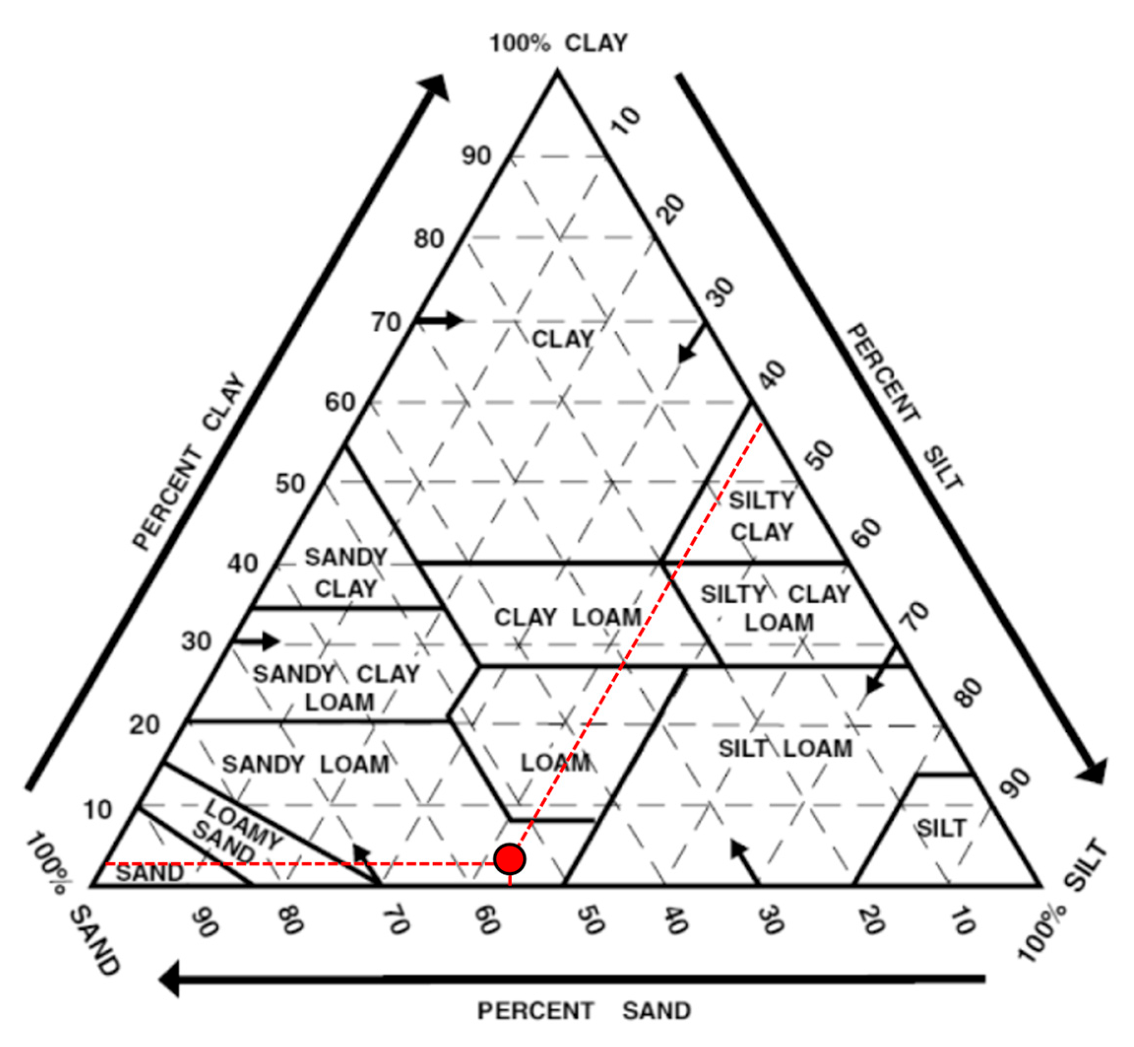
The soil texture of the samples used in this experiment was analyzed using the micro-pipette method and classified according to the USDA soil texture triangle [55]. The analysis indicates that the soil consists of 0.6% clay, 43% silt, and 56% sand.

As shown in Figure 2, the experimental soil falls in the sandy loam category on the USDA soil texture triangle on the basis of the above values.

2.2.3. Waterlogging Stress Treatment and Water Management

After plant acclimatization, the experiment was conducted using two treatment groups: a uniformly irrigated control group and a waterlogging treatment group, which was maintained in saturated conditions through surface waterlogging.

Angle-type drippers were used for irrigation by installing one dripper in each pot to deliver water directly to the soil through drip irrigation. During the acclimatization period, each potted plant was irrigated daily with 600 mL of water for 30 days. Waterlogging stress treatments were initiated once acclimatization was achieved following transplantation.

For the control group, we maintained the same irrigation regime used during plant acclimatization, supplying 600 mL of water daily per pot to sustain optimal moisture conditions. For the waterlogging treatment group, as shown in Figure 1b, each pot was placed inside a larger plastic container (referred to as a “living box”) to enable controlled waterlogging. Water was added to each container until it reached and slightly covered the soil surface of the pot, ensuring continuous soil saturation.

The water level was visually checked daily, and if it dropped below the soil surface due to evaporation or drainage, water was replenished as necessary to maintain surface saturation throughout the 30-day treatment period.

In each treatment group, two out of the four replicate pots (n = 2) were equipped with soil moisture sensors (WaterScout SM 100, Spectrum Technologies, Inc., Aurora, IL 60504, USA) inserted at a depth of 10 cm from the soil surface. Volumetric water content was recorded at one-hour intervals.

The moisture data that were recorded to track changes in soil moisture content were stored in a data logger (WatchDog 1000 Series Watermark Irrigation Micro Stations, Spectrum Technologies, Inc., Aurora, IL 60504, USA). Additionally, a digital thermo-hygrometer was used to monitor the temperature and the relative humidity inside the greenhouse at one-hour intervals (Testo 174 H, Titisee-Neustadt, Germany).

2.3. Data Measurement Methods

Multispectral Drone Imagery

A multispectral drone (Mavic 3 Multispectral, DJI Enterprise, Shenzhen, China) equipped with both an RGB camera and a multispectral camera was used to monitor changes in response to waterlogging stress among the experimental groups of the target plants. The RGB camera collected digital images in three bands: R445 (blue), R545 (green), and R650 (red). For the same image area, the multispectral camera acquired grayscale images at R560 ± 16 nm (green), R650 ± 16 nm (red), R730 ± 16 nm (red-edge), and R860 ± 26 nm (near-infrared). Five image replicates were acquired for each treatment group at a height of 3 m for the waterlogging stress experiment at 3, 6, 9, 12, 15, 20, and 30 days after treatment (DAT).

2.4. Image Data Processing

2.4.1. RGB Image Processing

RGB images collected through multispectral drone measurements were analyzed using the R software (ver. 4.3.2) environment [56]. Image preprocessing was performed using the R packages ‘FIELDimageR’ and ‘FIELDimageR.Extra’. The ‘fieldview’ function was used to assign the EPSG:4326 geographic coordinate system to the images. The region of interest (ROI) was defined for subsequent analysis.

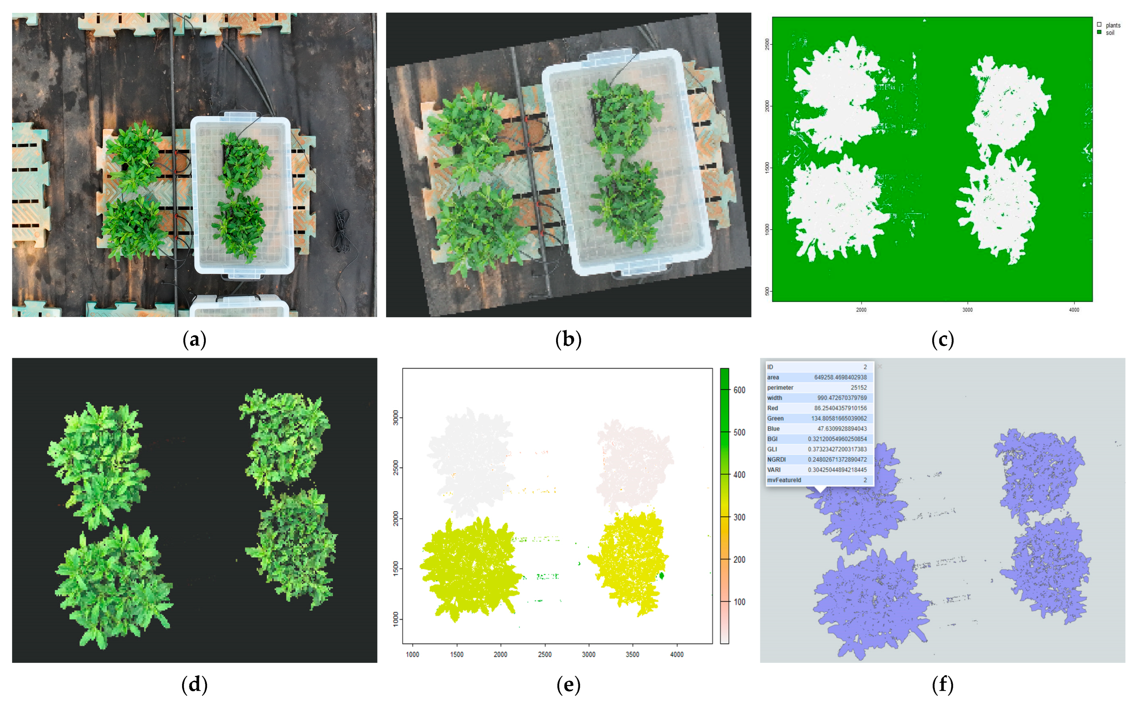
We implemented a supervised classification approach based on a random forest model to distinguish plant objects from the background. Representative training samples for both soil (background) and plant classes were manually selected from the mosaic image using the ‘fieldView’ function, with 1000 random points sampled for each class and labeled accordingly. The training samples were combined into a single dataset.

The ‘fieldSegment’ function was then applied to the mosaic image using the prepared training samples to perform supervised segmentation through the random forest algorithm. This process generated a classification model and predicted class labels for each pixel, resulting in a classified raster in which plant objects and background soil were clearly distinguished. The ‘fieldView’ and ‘plot’ functions visually inspected and verified the classification results.

Following background removal, the ‘fieldCount’ function was used to mask individual plant objects to enable the calculation of mean RGB image vegetation indices (RGB-VIs) for each object, including BGI, GLI, NGRDI, and VARI (

Table 1. Image preprocessing with FIELDimageR to generate vegetation indices.

Index	Description	Formula	Related Traits	References
BGI	Blue Green Pigment Index	B/G	Chlorophyll, Leaf Area Index (LAI)	[57]
GLI	Green Leaf Index	(2 × G − R − B)/(2 × G + R + B)	Chlorophyll	[58]
NGRDI	Normalized Green Red Difference Index	(G − R)/(G + R)	Chlorophyll, biomass, water content	[59]
VARI	Visible Atmospherically Resistant Index	(G − R)/(G + R − B)	Canopy, biomass, chlorophyll	[60]

). The overall workflow of the image processing procedure is illustrated in Figure 3.

2.4.2. Multispectral Image Processing

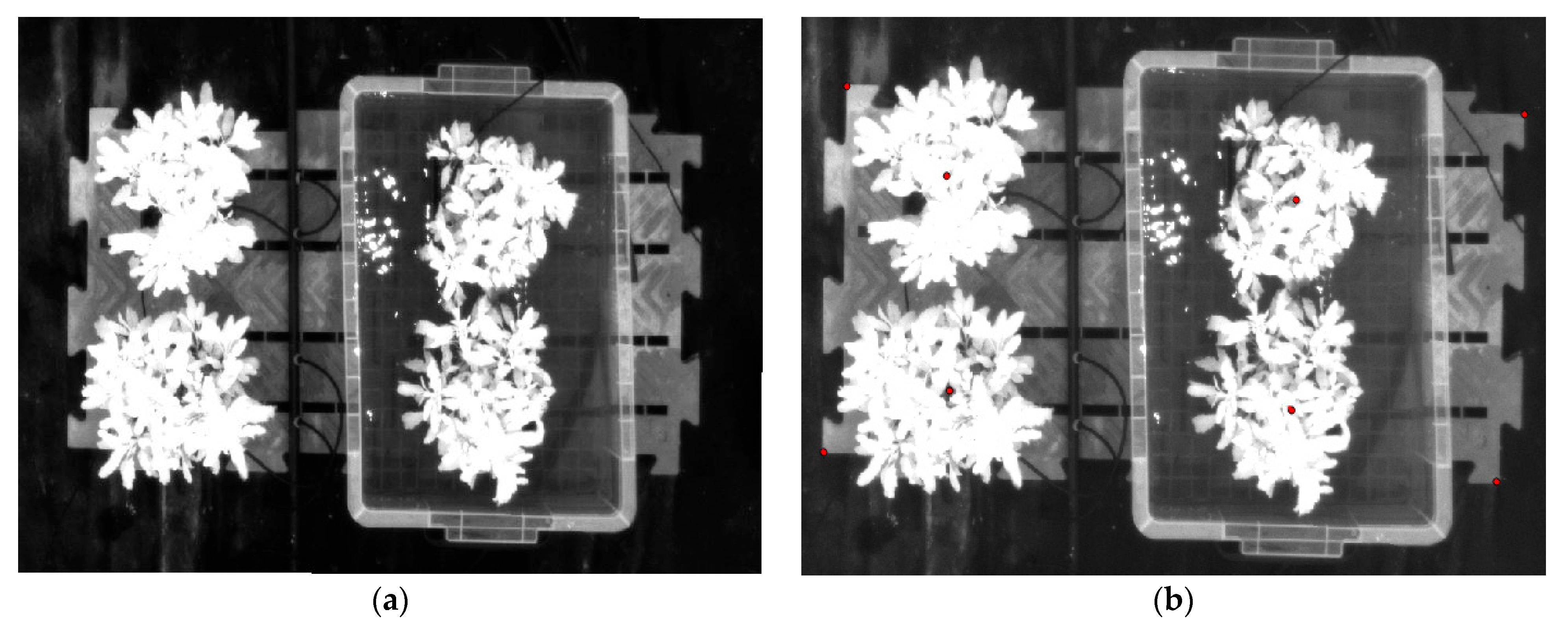
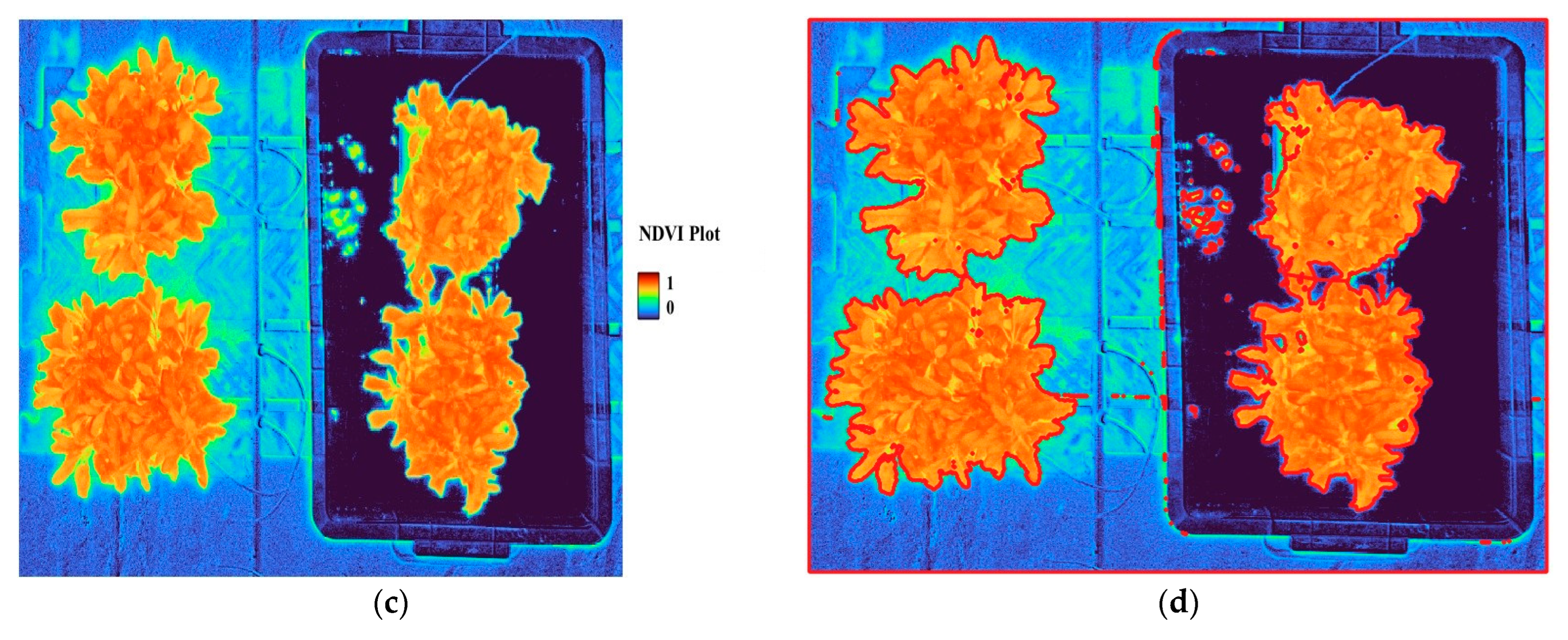
Multispectral images acquired with the multispectral camera were processed using R (ver. 4.3.2) and the Quantum Geographical Information System (QGIS ver. 3.42.1) [61]. Georeferencing was used to align the positions and orientations of the grayscale images for each wavelength. The aligned images were then used to calculate vegetation indices—specifically, NDVI and GNDVI—using the ‘raster calculator’ function in QGIS.

The resulting raster images were converted to vector format to delineate plant object boundaries as polygons. Using both the preprocessed raster and the vector images, we performed zonal statistics to extract vegetation index values (NDVI, GNDVI) for each plant object, including mean, variance, maximum, and minimum values (

Table 2. Vegetation indices calculated based on multispectral drone image processing.

Index	Description	Formula	References
GNDVI	Green NDVI	(RNIR − RGREEN)/(RNIR + RGREEN)	[62]
NDVI	Normalized Difference Vegetation Index	(RNIR − RRED)/(RNIR + RRED)	[63]

).

Furthermore, following the DJI Enterprise image processing guide [64], the raw grayscale image digital number (DN) values were radiometrically corrected using sensor metadata. Pixel values were converted to reflectance. The R packages ‘terra’ and ‘exifr’ were used to extract metadata for each band, including black level, gain, exposure time, and irradiance. Radiometric correction was performed using the following equations:

Radiance calculation for each pixel:

$$L={\displaystyle \frac{DN-BL}{k\times t}}$$

(1)

• DN: Digital Number of the pixel;
• BL: Sensor Black Level (or Dark Current);
• k: Sensor Gain;
• t: Exposure Time (µs).

Reflectance calculation:

$$\rho ={\displaystyle \frac{L\times GA}{E}}$$

(2)

• GA: Sensor Gain Adjustment;
• E: Irradiance (solar radiant energy).

Through this radiometric correction process, pixel values for each band were converted to actual reflectance values that were then used to calculate vegetation indices. The workflow for multispectral image processing is illustrated in Figure 4.

2.5. Statistical Analysis

All statistical analyses were performed using R software (version 4.3.2). To evaluate and predict waterlogging stress responses in P. linariifolium, one-way analysis of variance (ANOVA) was conducted to compare spectral vegetation indices, image-based indices (RGB-VIs), and soil moisture content among treatments. Duncan’s multiple range test was used to assess the significance of differences between treatments. Soil moisture content data were normalized using min–max scaling and analyzed based on cumulative values over the experimental period.

Correlation analysis and principal component analysis (PCA) were performed to identify optimal predictive variables among those displaying significant differences. The response patterns of control and waterlogging-treated groups were classified with hierarchical clustering analysis. Gower distance was calculated to handle mixed data types (categorical and continuous variables), and Ward’s method was used to merge clusters to minimize within-cluster variance. The optimal number of clusters was determined using the elbow method based on within-cluster sum of squares (WSS), and the results were visualized in a two-dimensional space. Silhouette analysis was used to evaluate the final clusters to see if they were adequate.

Based on the selected optimal variables, multiple regression analysis was performed to assess the relative impact of independent variables (spectral vegetation indices and image-based indices) on the dependent variable (cumulative volumetric soil moisture content) under conditions of waterlogging stress. The significance of each regression coefficient (p-value) was tested to identify independent variables with statistically significant effects on the dependent variable. Multicollinearity was assessed using the variance inflation factor (VIF). Variables with VIF greater than 10 were excluded from the model.

Model performance metrics and residual analysis were used to evaluate the overall fit of the multiple regression model. The normality of residuals was checked using a Q–Q plot, and homoscedasticity was examined using a residuals vs. fitted plot. All hypothesis tests were conducted at a significance level of 0.05.

3. Results

3.1. Environmental Changes During Water Management Treatments

3.1.1. Changes in Soil Moisture Content

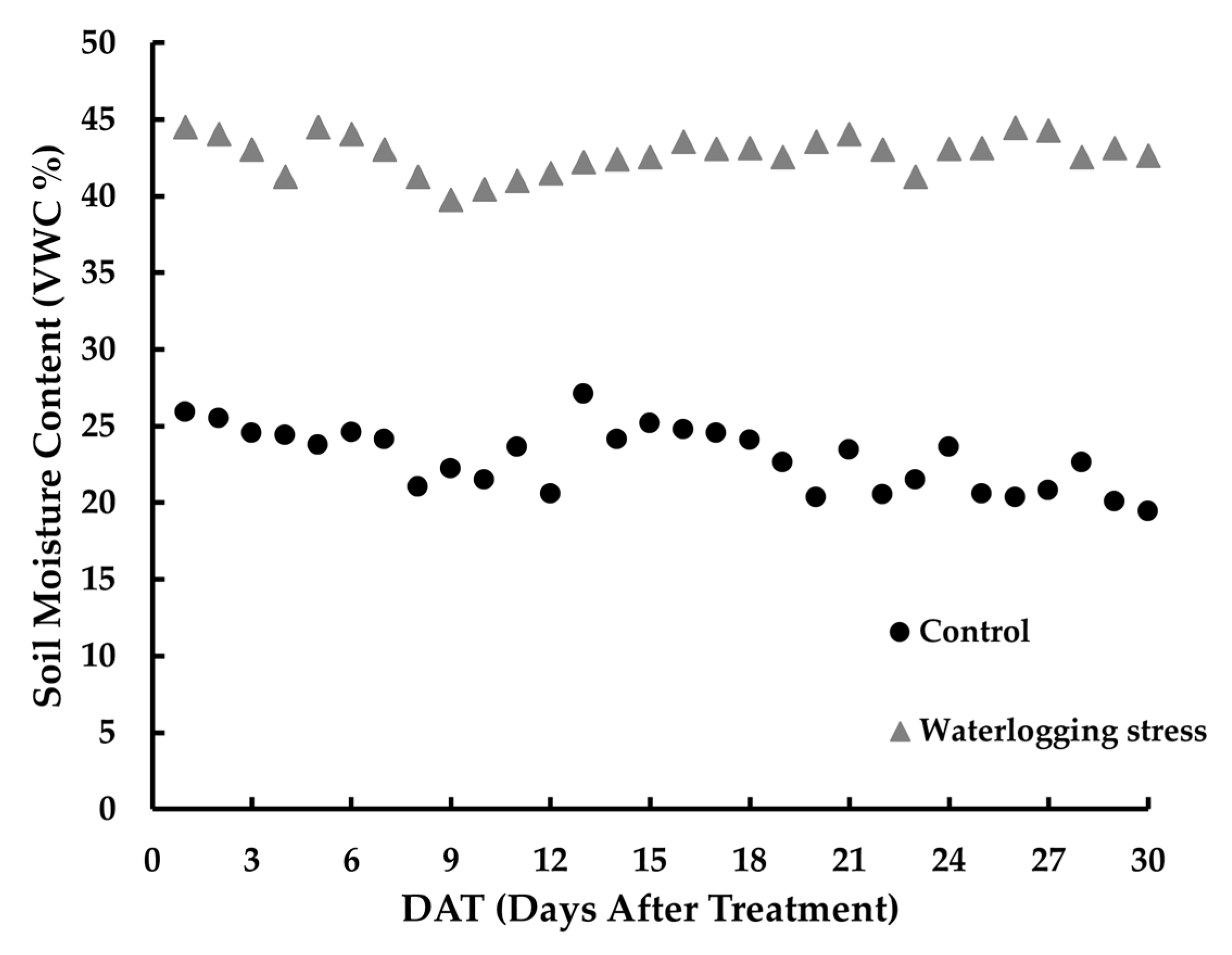
We investigated the responses to the stress of waterlogging in P. linariifolium under two treatment groups: (1) a uniformly irrigated control group and (2) a waterlogging treatment group. Each treatment group included four replicate pots (n = 4). The volumetric soil moisture content was monitored at one-hour intervals throughout the entire experimental period. The daily average values for each group are presented in Figure 5.

During the 30-day treatment period, the control group recorded maximum and minimum soil moisture levels of 27.07% and 19.44%, respectively, with an average soil moisture content of 22.91%. In contrast, we maintained saturated soil conditions in the waterlogging treatment group by ensuring that the soil surface in each pot remained submerged, with maximum, minimum, and average soil moisture contents of 44.5%, 39.7%, and 42.77%, respectively.

The minimum value obtained indicates that soil moisture in the waterlogging treatment group remained consistently above 39% (i.e., in a saturated state) for the duration of the experiment.

The cumulative volumetric soil moisture content (SM_Cum) showed clear differences between the control and waterlogging treatment groups over time (

Table 3. Cumulative volumetric soil moisture content (SM_Cum) measured at different days after treatment (DAT) under control and waterlogging stress conditions. Values represent the accumulation of volumetric water content over time, quantifying the intensity and duration of soil waterlogging stress applied in the experiment.

Treatment	Time	Cumulative Volumetric Soil Moisture Content
Control	3 DAT	0.701
	6 DAT	1.278
	9 DAT	1.637
	12 DAT	1.930
	15 DAT	2.652
	20 DAT	3.416
	30 DAT	4.157
Waterlogging Stress	3 DAT	2.924
	6 DAT	5.778
	9 DAT	8.402
	12 DAT	10.981
	15 DAT	13.728
	20 DAT	18.465
	30 DAT	27.933

). In the control group, SM_Cum gradually increased, reaching 4.16 by 30 DAT, while the waterlogging group exhibited a markedly higher accumulation, with SM_Cum rising sharply to 27.93 by 30 DAT, confirming sustained saturated soil conditions throughout the treatment period.

3.1.2. Changes in Temperature and Relative Humidity

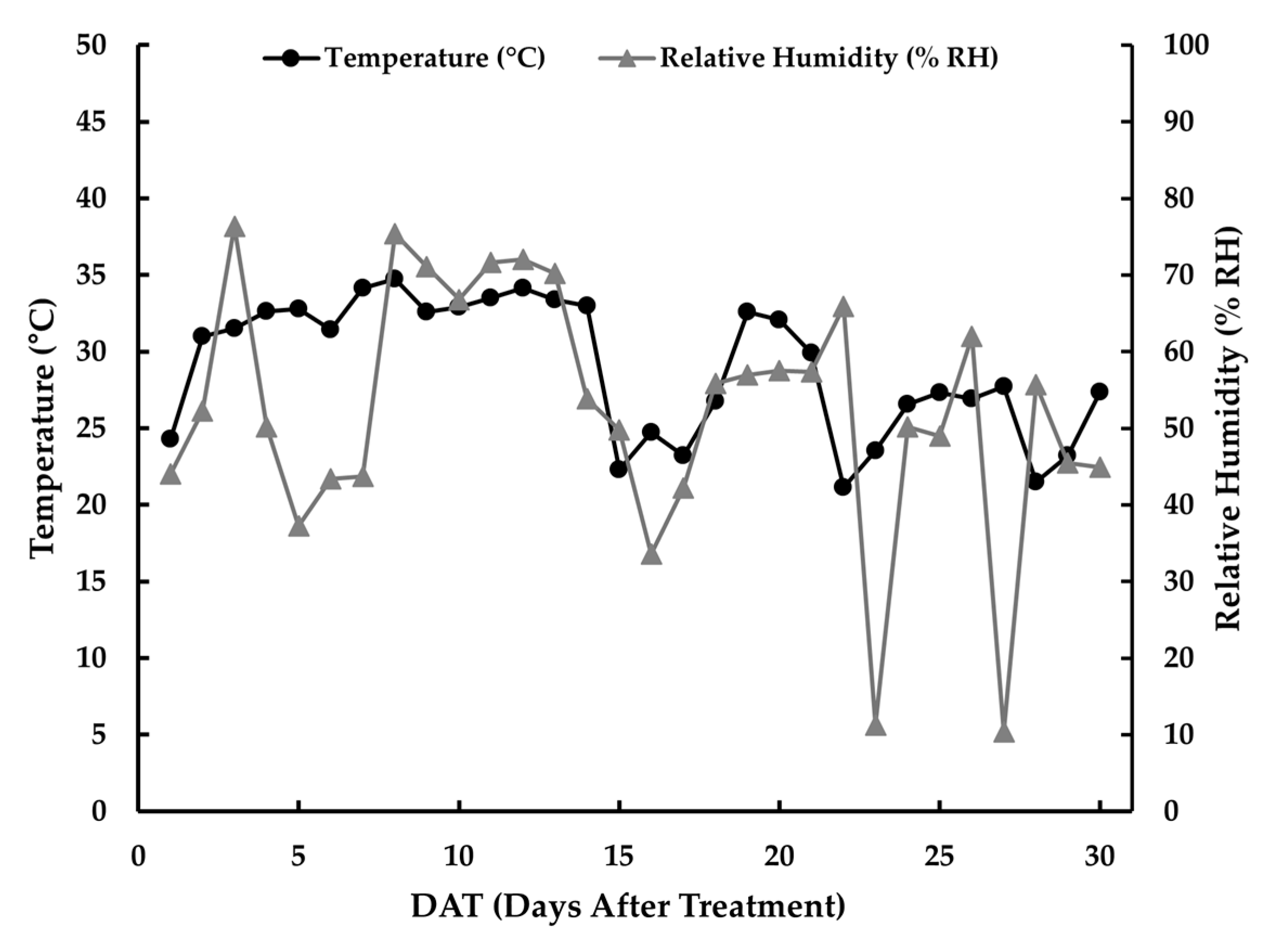
During the waterlogging stress experiment, we monitored air temperature and relative humidity in the experimental field at one-hour intervals. The daily average of the recorded temperature and relative humidity data are presented in Figure 6.

Over the course of the experiment, the average air temperature was 28.9 °C, with the highest daily average temperature reaching 34.7 °C and the lowest daily average falling to 21.1 °C. Although some fluctuations in relative humidity were observed throughout the experimental period, the average relative humidity was 52.5%.

3.2. Analysis of Waterlogging Stress Responses in P. linariifolium

3.2.1. Changes in RGB Image Vegetation Indices

To analyze RGB images obtained via multispectral drone imagery, a random forest model evaluated the stress responses to waterlogging in P. linariifolium by segmenting plant objects and eliminating the background. The model was trained with 685 image samples and validated using 5-fold cross-validation to achieve high classification reliability, with an accuracy of 94.72% and a Kappa value of 0.894. The processed images were used to calculate four vegetation indices: BGI, GLI, NGRDI, and VARI.

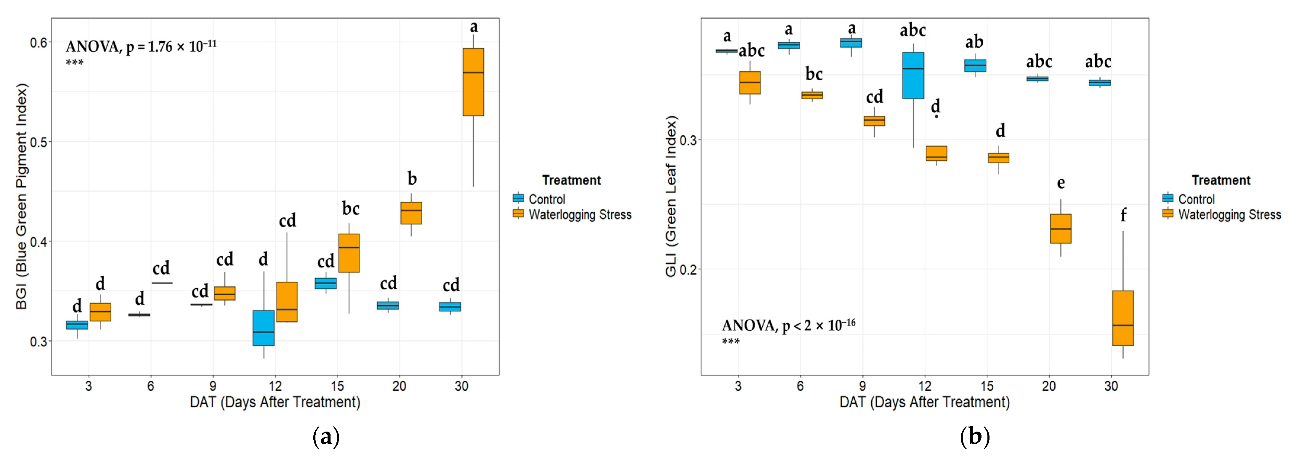
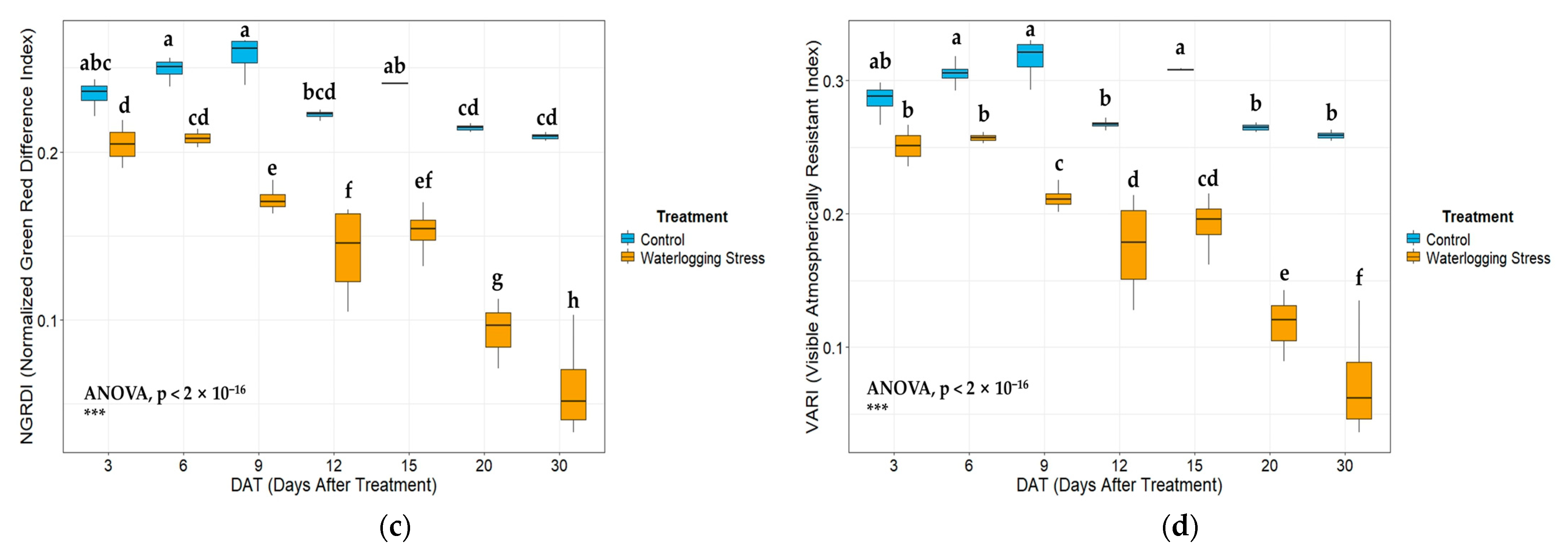
In the control group, these vegetation indices remained relatively stable throughout the experimental period. The GLI values ranged from 0.29 to 0.38, starting with 0.36 on the third Day After Treatment (DAT). The NGRDI varied between 0.21 and 0.26, registering values of 0.23 at 3 DAT and 0.21 at 30 DAT. The VARI fluctuated from 0.25 to 0.33, beginning with 0.28 at 3 DAT, while BGI was consistently maintained between 0.28 and 0.37, with an initial value of 0.32 at 3 DAT.

In the waterlogging-treated group (WL), we observed marked changes in vegetation indices after 6 DAT. The GLI values decreased from 0.34 at 3 DAT to 0.16 at 30 DAT, corresponding to a decrease of 52.9%. Over the same period, NGRDI values also decreased by dropping from 0.22 to 0.09—a reduction of 59.1%. Similarly, the values of VARI fell from its initial value of 0.26 after 6 DAT to 0.06 at 30 DAT, representing a 77.8% decrease.

In contrast to these trends, BGI values increased from 0.34 at 3 DAT to 0.61 at 30 DAT, reflecting a 79.4% increase. Statistically significant differences between the WL and the control groups began to emerge as early as 6 DAT for several indices and became much more pronounced after 15 DAT.

In Figure 7, the boxplots display the time-dependent trends for each vegetation index in both the groups. The figure shows that the values of GLI, NGRDI, and VARI reduced significantly under the persistent stress of waterlogging, reflecting reduced chlorophyll content and biomass, while BGI values exhibited a marked increase compared to those in the control.

These physiological changes became more pronounced after 15 DAT, underscoring the progressive impact of waterlogging over time on the spectral traits of P. linariifolium.

3.2.2. Changes in NDVI and GNDVI Based on Multispectral Imaging

The QGIS was used to process multispectral images to evaluate the effects of the stress of waterlogging on the growth and physiological responses of P. linariifolium. NDVI and GNDVI were calculated from these images to assess the vegetation status under different treatment conditions.

Both indices showed a consistent decreasing trend over time in the WL group, with GNDVI exhibiting a greater rate of decline than NDVI. In contrast, despite minor fluctuations, the control group maintained relatively stable values for both indices throughout the experimental period.

From approximately 10 DAT, one control individual began exhibiting abnormal stress symptoms due to irrigation failure and pest infestation. Therefore, this individual was excluded from image analysis and statistical evaluation from 12 DAT onward.

Table 4. Temporal changes in NDVI and GNDVI values of control and waterlogging-treated (WL) groups during the experimental period of 30 days.

Vegetation Index	Time	Treatment
		Control	Waterlogging Stress
NDVI ***	3 DAT	0.716 ± 0.018 cde	0.720 ± 0.003 bcde
	6 DAT	0.743 ± 0.014 ab	0.719 ± 0.023 bcde
	9 DAT	0.746 ± 0.009 a	0.709 ± 0.008 de
	12 DAT	0.742 ± 0.003 ab	0.699 ± 0.008 ef
	15 DAT	0.736 ± 0.004 abc	0.684 ± 0.003 f
	20 DAT	0.726 ± 0.013 abcd	0.613 ± 0.033 g
	30 DAT	0.711 ± 0.011 de	0.568 ± 0.014 h
GNDVI ***	3 DAT	0.594 ± 0.013 ab	0.580 ± 0.004 abc
	6 DAT	0.590 ± 0.002 abc	0.573 ± 0.002 bcd
	9 DAT	0.594 ± 0.011 ab	0.567 ± 0.007 cd
	12 DAT	0.591 ± 0.002 abc	0.566 ± 0.005 cd
	15 DAT	0.585 ± 0.005 abc	0.555 ± 0.006 d
	20 DAT	0.599 ± 0.011 a	0.403 ± 0.012 e
	30 DAT	0.596 ± 0.006 ab	0.379 ± 0.041 f

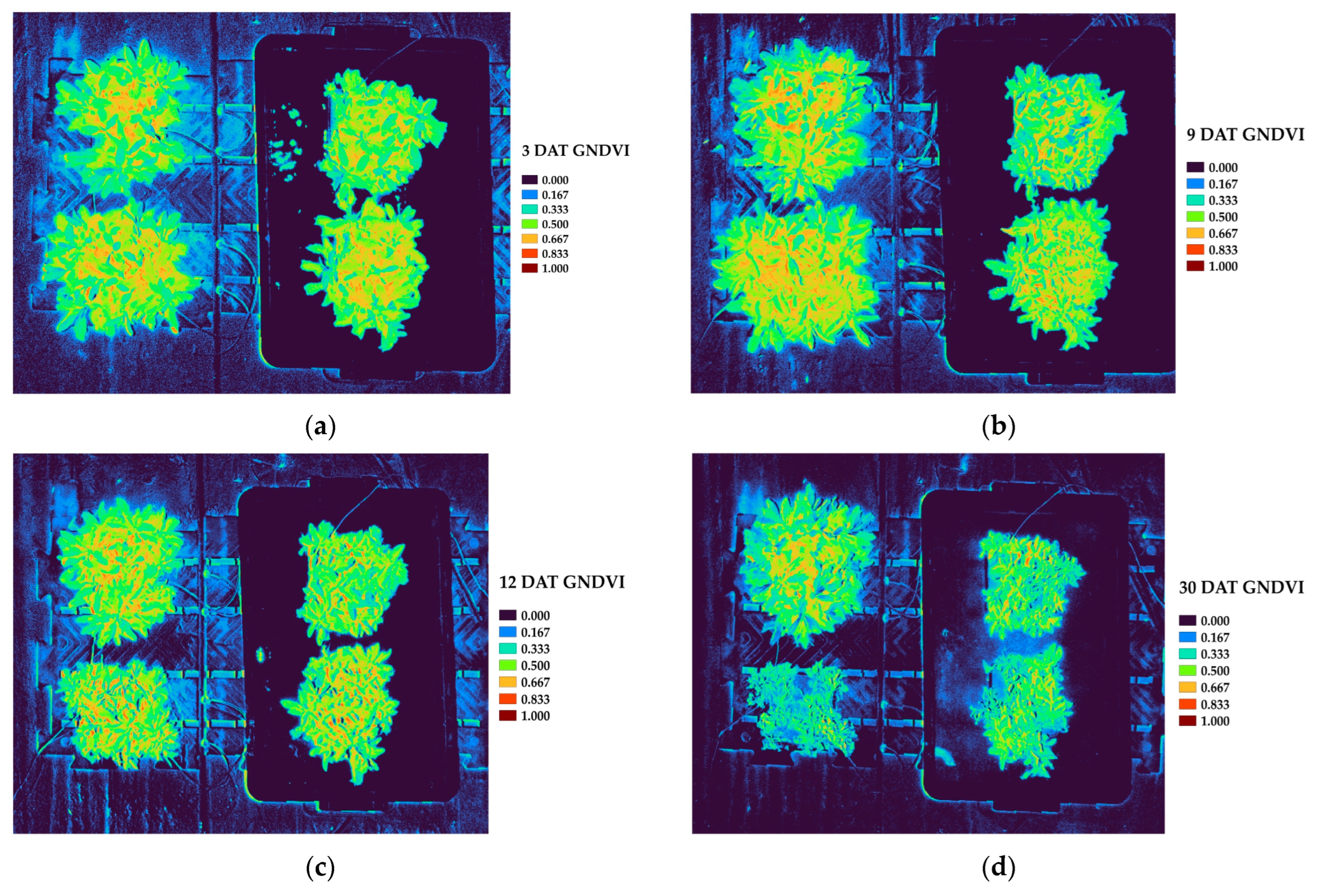
Note: Values represent mean ± standard deviation. Different letters within each row indicate significant differences between treatments and time points at p < 0.05, according to Duncan’s multiple range test; groups sharing the same letter are not significantly different. Statistical significance was determined by one-way ANOVA (*** p < 0.001).

summarizes the temporal changes in NDVI and GNDVI. In the WL group, NDVI was significantly lower than that in the control as early as 6 days after treatment (DAT) (p < 0.05). The differences between the groups became even more pronounced beginning from 9 DAT. The NDVI continued to decline gradually up to 15 DAT, followed by a sharp reduction, with a total decline of more than 21% by 30 DAT. For GNDVI, we did not detect any significant difference at 6 DAT, but from 9 DAT onwards, the WL group exhibited significantly lower values than those of the control (p < 0.05). The GNDVI continued to decrease through 15 DAT and showed a reduction of over 34% by 30 DAT.

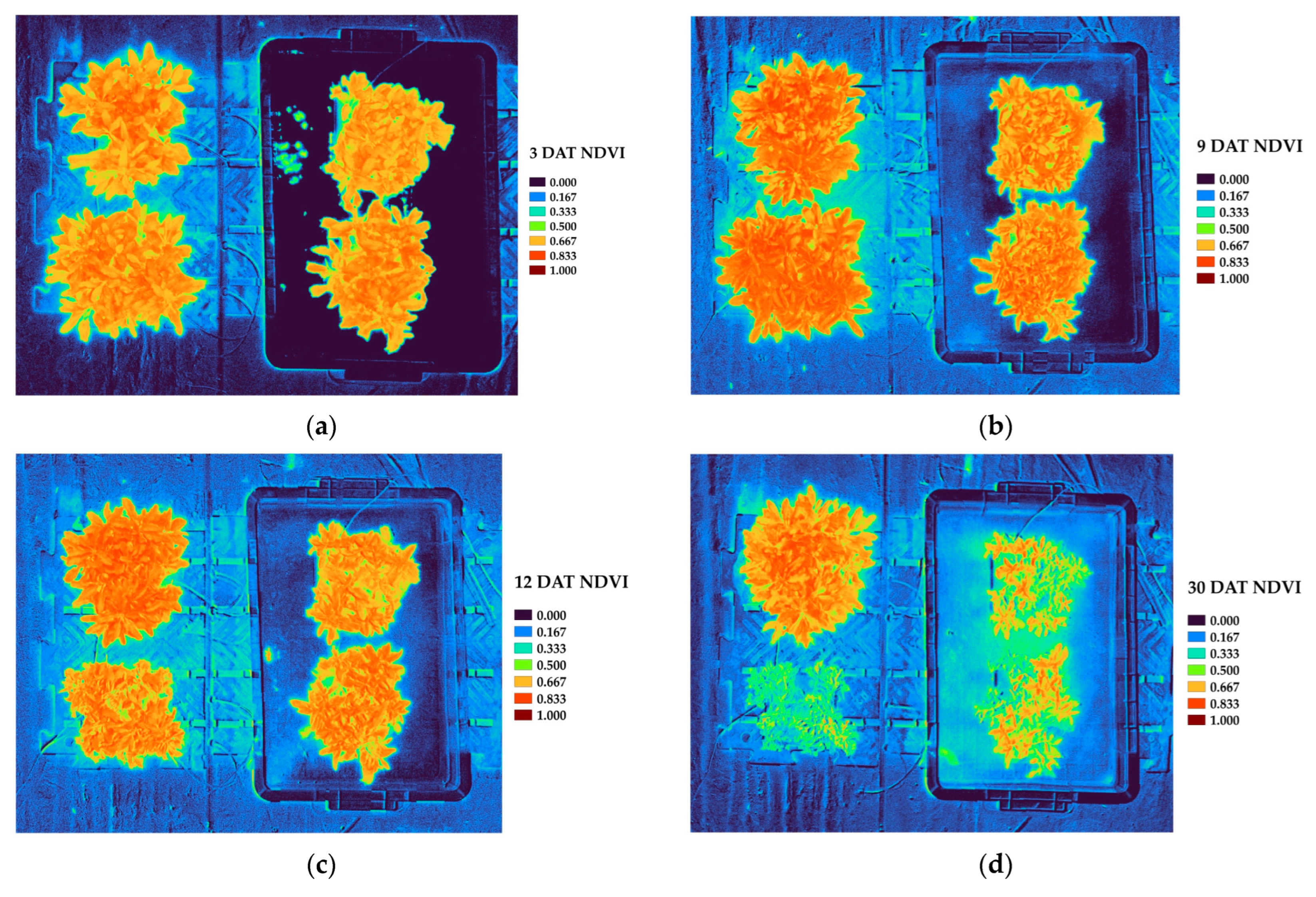
Figure 8 and Figure 9 exhibit these time-dependent trends, which display multispectral images showing spatial distributions of NDVI and GNDVI at selected time points (3, 9, 12, and 30 DAT). In each image, the left side shows the control group, and the right side depicts the WL group. Both indices remained high and stable in the control group, whereas the values of NDVI and GNDVI in the WL group progressively decreased as the stress of waterlogging persisted (Supplementary Materials). The most prominent differences appear at 30 DAT, as confirmed by the quantitative results in Table 3.

Statistical significance was assessed using one-way ANOVA followed by Duncan’s multiple range test. Different letters in Table 3 and Figure 8 and Figure 9 indicate significant differences between treatments and time points at p < 0.05. Significance levels are denoted as follows: *** p < 0.001.

3.3. Evaluation of Waterlogging Stress and Selection of Predictive Variables Using Non-Destructive Analysis

3.3.1. Selection of Optimal Predictive Variables

Correlation Analysis

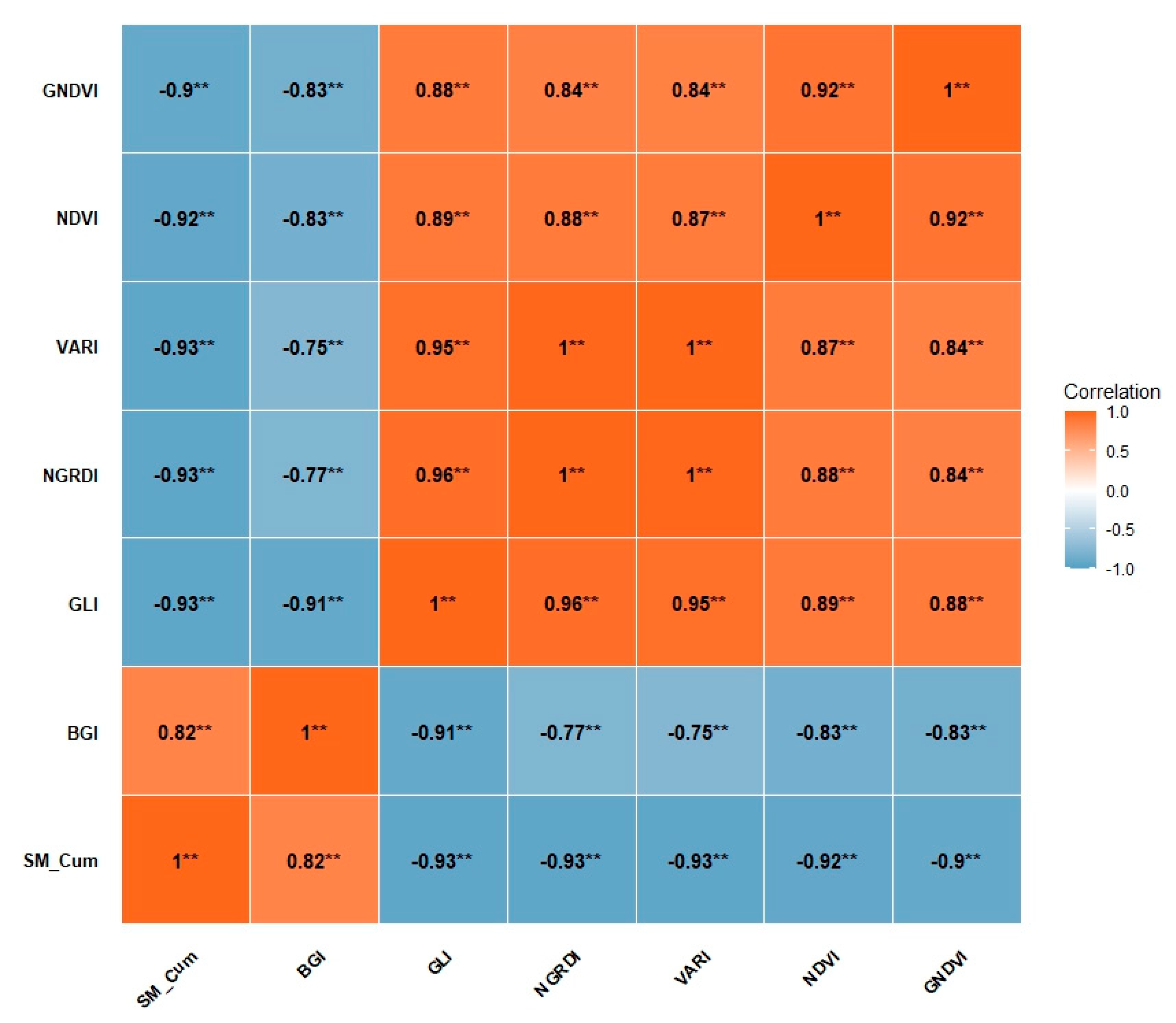
To identify optimal predictive variables that can assess waterlogging stress in P. linariifolium, Pearson correlation analysis was conducted between Cumulative volumetric Soil Moisture content (SM_Cum) and various vegetation indices. The Shapiro–Wilk test was used to confirm data normality. Statistically significant correlation coefficients (p < 0.05) were visualized in a correlation matrix (Figure 10).

SM_Cum showed strong and significant negative correlations with NDVI (r = −0.92 **) and GNDVI (r = −0.90 **), indicating that high levels of waterlogging are associated with reduced plant vigor and photosynthetic activity.

Among RGB-based indices, GLI (r = −0.93 **), NGRDI (r = −0.93 **), and VARI (r = −0.93 **) also demonstrate strong negative correlations, while BGI showed a significant positive correlation (r = 0.82 **). These results demonstrate a clear relationship between soil moisture status and changes in multiple vegetation indices when subjected to the stress of waterlogging.

Based on these correlation results, indices with an absolute correlation coefficient above 0.7 were selected as candidate variables for further multivariate analysis. We subsequently performed principal component analysis (PCA) and variance inflation factor (VIF) assessments to address potential multicollinearity and redundancy among the selected variables.

Principal Component Analysis (PCA)

To select optimal predictive variables for waterlogging stress in P. linariifolium, principal component analysis (PCA) was performed on the set of indices previously identified by Pearson correlation analysis. This multivariate approach helped to determine relationships among variables, to enable the extraction of key underlying patterns, and to identify two principal components (PC1 and PC2). Cluster ellipses in the PCA plot helped to visualize group differences (Figure 11).

PCA revealed that the first two principal components collectively explained 94.9% of the total variance, with PC1 accounting for 90.1% and PC2 explaining an additional 4.8%.

Table 5. Loadings of each variable on PC1 and PC2 from principal component analysis.

Variable	PC1	PC2
SM_Cum	0.3862	−0.1004
GLI	−0.3906	−0.0014
NGRDI	−0.3828	0.4437
VARI	−0.3805	0.4807
BGI	0.3533	0.6902
NDVI	−0.3786	−0.1314
GNDVI	−0.3726	−0.2613

lists the loadings of variables for each component, where larger absolute values indicate greater contributions to the corresponding principal component.

Upon examining the loadings, GLI (−0.39), NGRDI (−0.38), VARI (−0.38), NDVI (−0.38), and GNDVI (−0.37) demonstrated strong negative loading on PC1, indicating that these indices are key contributors that define the control group. In contrast, BGI (0.35) and Cumulative volumetric Soil Moisture content (SM_Cum, 0.39) exhibited positive loadings on PC1, reflecting their strong association with the WL group. BGI had the largest positive loading (0.69) on PC2, suggesting its heightened variability under waterlogging conditions.

The PCA plot (Figure 11) clearly illustrates these findings: the control group (red dots) clustered to the left along PC1, while the WL group (blue dots) showed a wide distribution to the right. This spatial separation is consistent with high values for GLI, NGRDI, VARI, NDVI, and GNDVI under normal growth conditions, and an increase in BGI and sm_cum values under waterlogged conditions.

Based on the combined Pearson correlation and PCA results, six vegetation indices—NDVI, GNDVI, GLI, BGI, NGRDI, and VARI—were selected as optimal predictive variables to evaluate the stress due to waterlogging in P. linariifolium. This selection is supported by their clear and differential responses to stress and provides an objective basis for future modeling and monitoring.

3.3.2. Classification of Waterlogging Stress by Clustering

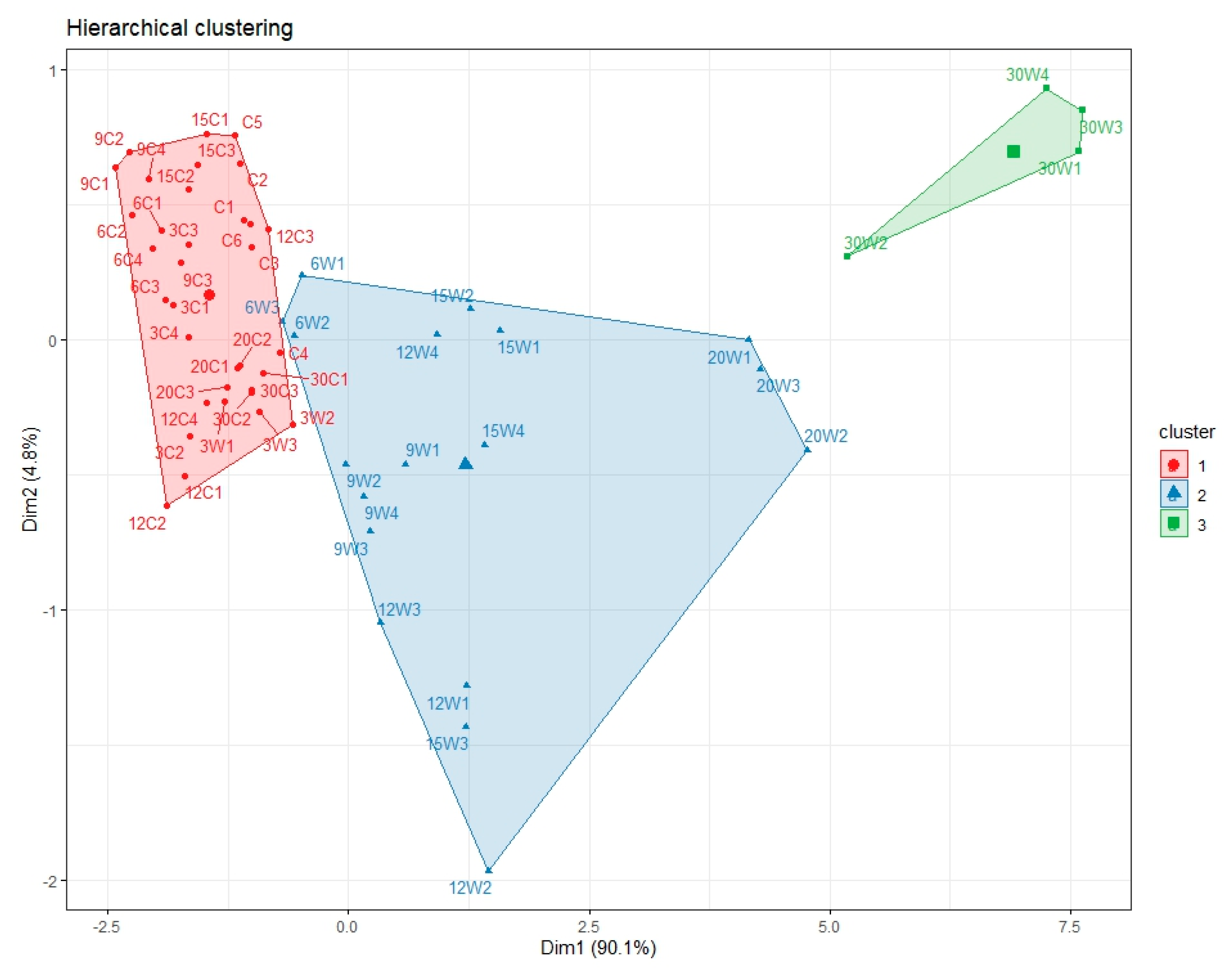
We performed hierarchical clustering analysis to further differentiate the distribution patterns between the control and the WL groups. The optimal number of clusters (k) was determined using an elbow plot of the within-cluster sum of squares (WSS), where a clear elbow was observed at k = 3. Thus, three clusters were selected for the analysis.

The clustering analysis revealed three distinct groups that corresponded well to the treatment conditions and the temporal progression of waterlogging stress. Samples in Cluster 1 were primarily from the control group and exhibited a densely grouped distribution across various time points, including 3, 6, 9, 12, 15, 20, and 30 DAT. This indicates that the control group maintained a relatively stable physiological state throughout the experiment by forming a consistently compact and independent cluster, irrespective of treatment duration.

Cluster 2 included most early- to mid-stage waterlogging samples, notably, from 6 to 20 days after treatment (DAT). These samples occupy an intermediate position between the control and late-stage WL samples, representing a physiological transition phase as stress responses begin to emerge and intensify with sustained waterlogging.

In contrast, Cluster 3 consisted of late-stage waterlogging samples collected at 30 DAT, which formed a well-separated group in the ordination space. The distinct spatial isolation and spread of this cluster reflect a marked divergence in physiological state after prolonged waterlogging, consistent with the late stress trajectories observed in PCA.

Figure 12 shows the distribution patterns and group separations, where clear stratification among the clusters is evident and reflects differences in the physiological status across conditions and time points.

To assess clustering validity, silhouette analysis was performed. The results demonstrated that more than 75% of samples had silhouette widths above 0.6, indicating that clusters were generally well separated and appropriately assigned. This confirms the reliability of the clustering approach to distinguish physiological responses to waterlogging stress in P. linariifolium.

Overall, hierarchical clustering provided clear and interpretable groupings to support the classification of plant responses according to the treatment group and the progression of stress.

3.3.3. Multiple Linear Regression Analysis and Prediction Model Development

To evaluate the relative contributions of vegetation indices to SM_Cum, a multiple linear regression analysis was conducted using the previously selected variables. During variable selection, multicollinearity was assessed using the variance inflation factor (VIF). Variables with VIF values exceeding 10—specifically, BGI (18.95), GLI (74.46), NGRDI (246.64), and VARI (222.27)—were excluded due to severe multicollinearity. As a result, NDVI (VIF = 4.89) and GNDVI (VIF = 5.15) were retained in the final model because they were both within acceptable thresholds.

Table 6. Regression coefficients, standard errors, t-values, p-values, and VIF for the final multiple linear regression model to predict SM_Cum using NDVI and GNDVI.

Variable	Estimate	Std. Error	t-Value	p-Value	VIF
Intercept	66.486	2.909	22.855	<0.001	-
NDVI	−45.774	7.023	−6.518	<0.001	3.14
GNDVI	−56.194	9.162	−6.133	<0.001	3.14

Note: VIF (variance inflation factor) values below 10 indicate that multicollinearity is not significant in the final model. All p-values < 0.05 are considered statistically significant.

summarizes the regression results. Both NDVI (estimate = −45.774, p < 0.001) and GNDVI (estimate = −56.194, p < 0.001) showed statistically significant negative coefficients, indicating that low values of these indices are associated with increased soil moisture under waterlogged conditions. The final regression equation is presented in Equation (3):

$$\mathit{C}\mathit{u}\mathit{m}\mathit{u}\mathit{l}\mathit{a}\mathit{t}\mathit{i}\mathit{v}\mathit{e} \mathit{v}\mathit{o}\mathit{l}\mathit{u}\mathit{m}\mathit{e}\mathit{t}\mathit{r}\mathit{i}\mathit{c} \mathit{S}\mathit{o}\mathit{i}\mathit{l} \mathit{M}\mathit{o}\mathit{i}\mathit{s}\mathit{t}\mathit{u}\mathit{r}\mathit{e} \mathit{c}\mathit{o}\mathit{n}\mathit{t}\mathit{e}\mathit{n}\mathit{t}=-45.774\times \mathit{N}\mathit{D}\mathit{V}\mathit{I}-56.194\times \mathit{G}\mathit{N}\mathit{D}\mathit{V}\mathit{I}+66.486$$

(3)

The predictive performance of the multiple linear regression model was evaluated using several diagnostic metrics. As presented in

Table 7. Performance and diagnostic summary of the final multiple linear regression model to predict SM_Cum.

Indicator	Value
R2	0.8966
Adjusted R2	0.8927
RMSE	2.4927
MAE	2.0234

Abbreviations: R²—coefficient of determination; RMSE—root mean squared error; MAE—mean absolute error.

, the model achieved an R² value of 0.8966 and an adjusted R² of 0.8927, indicating that approximately 90% of the variation in SM_Cum could be explained by the model. The RMSE and MAE were 2.4927 and 2.0234, respectively, which suggested minimal prediction errors.

To verify the adequacy of the model, residual diagnostics were conducted via a Q–Q plot and a residuals-versus-fitted plot (Figure 13). The Q–Q plot showed that most residuals aligned closely along the reference line, confirming the normality assumption. The residuals-versus-fitted plot displayed a random scatter without a discernible structure. This supported the assumption of homoscedasticity. Together, these findings indicate that the regression model is statistically robust and can serve as a reliable tool to predict waterlogging stress in P. linariifolium.

4. Discussion

Our study quantitatively evaluated the physiological responses of P. linariifolium to the stress of waterlogging using a non-destructive, image-based approach and identified key predictive variables. Various vegetation indices were calculated from RGB and multispectral imagery acquired by drones. The vegetation indices were then analyzed in combination with soil moisture data recorded by sensors. Unlike conventional physiological and biochemical analyses, this approach allows for consistent monitoring and offers potential applicability in field conditions. The results reaffirm the effectiveness of image-based evaluation methods [65,66,67].

Waterlogging is representative of environmental stress that cuts off the oxygen supply to the soil and suppresses root respiration [68,69,70,71], leading to an overall decline in physiological function [56,57,58]. In the present study, we observed a gradual decline in the growth status of P. linariifolium with the increasing duration of waterlogging. This indicates progressive accumulation of the physiological effects of waterlogging over time. A significant reduction in the aboveground traits, such as leaf area and chlorophyll content—indirectly inferred from changes in vegetation indices—suggest the potential of image-based monitoring to evaluate stress-induced physiological responses and to confirm the validity of image-derived quantification.

Soil moisture measurements showed that the control maintained an average moisture content of 22.91%, whereas the waterlogging treatment consistently maintained high levels close to saturation, which averaged 42.77%. These contrasting moisture conditions likely functioned as a clear physical stress factor that is potentially related to inhibited root respiration and oxygen deprivation [23,24,72,73]. Distinct physiological differences between the control and the treatment groups appeared after 6 DAT, indicating that the stress response accumulates over time before manifesting [22].

In the vegetation index analysis, key indices that include NDVI, GNDVI, GLI, VARI, and NGRDI exhibited declining trends under waterlogged conditions. The physiological suppression induced by stress is effectively reflected by the significantly low values of NDVI and GNDVI in waterlogged plots, which are closely correlated with photosynthetic activity and chlorophyll content [63,74,75].

NDVI and GNDVI are widely recognized for their sensitivity to chlorophyll concentration and photosynthetic capacity, making them reliable indicators of plant vigor and stress-induced functional decline [76,77,78]. RGB-based indices such as GLI, NGRDI, and VARI assess changes in reflectance within the visible spectrum, capturing alterations in leaf coloration associated with chlorophyll degradation, chlorosis, and yellowing, thus providing early, non-destructive markers of physiological stress [79,80]. Conversely, BGI quantifies increases in brownish pigments related to tissue senescence and damage [57], reflecting advanced stages of waterlogging stress.

The gradual decline in vegetation index values over time under continuous waterlogging is consistent with previous findings of excess moisture that negatively affects plant growth [81,82,83,84,85]. Our findings reinforce the utility of image-based remote sensing as a tool to capture the temporal and spatial dynamics of plant stress.

Correlation analysis indicated significant negative relationships between cumulative volumetric soil moisture and key vegetation indices. This result suggests a strong link between soil water levels and plant health status [86,87,88], emphasizing the importance of water management as a factor that directly influences plant growth.

Principal component analysis (PCA) results showed that major vegetation indices were strongly associated with the first principal component (PC1) and were clearly separated according to waterlogging treatment. High values of indices, such as NDVI, GNDVI, and VARI, were representative of the control group cluster, and the high values of BGI and accumulated soil moisture were associated with the waterlogged group cluster. These results confirm that the vegetation indices show distinct patterns in a multidimensional space under stress conditions [89], indicating their usefulness as classification tools to distinguish stress environments.

Hierarchical clustering analysis identified three main clusters corresponding to three distinct stress levels over time. Early- and late-stage stress groups were clearly differentiated from the control, with cluster boundaries becoming more distinct after 9 DAT. This suggests that physiological responses to waterlogging are cumulative over time and may become irreversible beyond a certain point.

The final multiple regression model, using only NDVI and GNDVI as predictors, explained 89.7% of the cumulative volumetric water content. The multiple regression model fulfilled all the assumptions of linear regression, including normality and homoscedasticity. This highlights the potential to construct high-quality predictive models using non-destructive image-derived data, which contributes to the automation and refinement of field monitoring systems [90]. Furthermore, since NDVI and GNDVI are widely applicable across both satellite and UAV platforms, their compatibility supports broad implementation in future monitoring frameworks with improved spatial resolution and sensor diversity.

Despite the promising predictive ability of the model, it is recognized that the model’s structure and variables included have limitations. Multicollinearity was carefully addressed by excluding variables with high VIF values, and the final model retained NDVI and GNDVI with acceptable VIFs. However, other potentially influential environmental or physiological variables were not included due to data constraints. Future improvements should be explored by incorporating additional relevant variables and advanced modeling techniques to enhance prediction accuracy and robustness under diverse field conditions.

Our study provides baseline data to quantify the stress response of ornamental or non-crop species like P. linariifolium through image-based methods. Our findings may serve as a helpful reference to develop management systems for urban green spaces or garden plants. Nevertheless, our study has the following limitations: (1) a semi-controlled greenhouse, where soil moisture was precisely controlled to simulate waterlogging stress, while ambient environmental conditions were relatively natural; (2) physiological metrics like leaf temperature or stomatal conductance were not simultaneously measured; and (3) only specific growth stages were evaluated. Future research should focus on repetitive experiments under outdoor conditions and adopt strategies that integrate multiple stress factors and developmental stages.

We acknowledge that urban environments present complex challenges—notably, varying microclimates, background noise, and other abiotic stressors—that were not fully replicated in our semi-controlled greenhouse setup. These limitations are addressed in the manuscript. Future research will focus on long-term, repetitive field experiments in diverse urban settings to enhance model robustness and applicability under multiple stresses. Moreover, strategic integration of multiple stress factors and developmental stages will be critical for comprehensive assessments.

5. Conclusions

Our study utilized a non-destructive analysis of multispectral drone imagery to quantitatively assess changes in vegetation indices of P. linariifolium under the stress of waterlogging in a greenhouse environment. As the duration of the stress of waterlogging increased, we observed significant decreases in key spectral vegetation indices, such as NDVI and GNDVI, reflecting reduced photosynthetic capacity and chlorophyll content.

Importantly, our research demonstrates that waterlogging responses in urban ornamental forbs like P. linariifolium can be rapidly monitored using drone-based multispectral imagery. Our findings offer valuable foundational data that can form the basis for technologies that advance urban green space management and garden plant maintenance.

However, our study is limited by its focus on short-term waterlogging treatments under semi-controlled greenhouse conditions and the absence of long-term monitoring throughout the entire growing period. Future research should address these limitations with repetitive experiments in open-field conditions and incorporate a wide range of environmental factors and physiological indicators for comprehensive, long-term assessment.

References

1. Speak, A.; Rothwell, J.; Lindley, S.; Smith, C. Urban particulate pollution reduction by four species of green roof vegetation in a UK city. Atmos. Environ. 2012, 61, 283–293. [Google Scholar] [CrossRef]
2. Kabisch, N.; Qureshi, S.; Haase, D. Human–environment interactions in urban green spaces—A systematic review of contemporary issues and prospects for future research. Environ. Impact Assess. Rev. 2015, 50, 25–34. [Google Scholar] [CrossRef]
3. Goddard, M.A.; Dougill, A.J.; Benton, T.G. Scaling up from gardens: Biodiversity conservation in urban environments. Trends Ecol. Evol. 2010, 25, 90–98. [Google Scholar] [CrossRef]
4. Plants of the World Online; Royal Botanic Gardens, Kew. Available online: https://powo.science.kew.org/taxon/urn:lsid:ipni.org:names:808505-1 (accessed on 21 July 2025).
5. National Institute of Biological Resources (NIBR). Korean Biodiversity Information System. Available online: https://species.nibr.go.kr/species/speciesDetail.do?ktsn=120000063333 (accessed on 21 July 2025).
6. Xue, H.; Liu, J.; Ma, G.; Zhou, X.; Sun, L.; Shi, Y.; Zhu, W.; Chen, K.; Zhang, L.; Li, Y. Phenols and γ-Lactams from the Aerial Part of Pseudolysimachion linariifolium subsp. dilatatum. Chem. Biodivers. 2020, 17, e2000387. [Google Scholar] [CrossRef]
7. Xue, H.-B.; Wang, P.; Wu, L.; Qian, F.; Chen, K.-X.; Zhang, L.-Q.; Li, Y.-M. Seven diastereomeric aucubigenin derivatives from Pseudolysimachion linariifolium subsp. dilatatum. J. Mol. Struct. 2022, 1264, 133303. [Google Scholar] [CrossRef]
8. King, C.M.; Robinson, J.S.; Cameron, R.W. Flooding tolerance in four ‘Garrigue’ landscape plants: Implications for their future use in the urban landscapes of north-west Europe? Landsc. Urban Plan. 2012, 107, 100–110. [Google Scholar] [CrossRef]
9. Gattringer, J.P.; Donath, T.W.; Eckstein, R.L.; Ludewig, K.; Otte, A.; Harvolk-Schöning, S. Flooding tolerance of four floodplain meadow species depends on age. PLoS ONE 2017, 12, e0176869. [Google Scholar] [CrossRef]
10. Liu, M.; Zhang, Q.; Xu, J.; Bao, M.; Zhang, D.; Xie, A.; Sun, X. Effects of waterlogging stress on the physiological characteristics and secondary metabolites of Herbaceous Peony (Paeonia lactiflora Pall.). Am. J. Plant Sci. 2021, 12, 536. [Google Scholar] [CrossRef]
11. Zhang, X.-M.; Duan, S.-G.; Xia, Y.; Li, J.-T.; Liu, L.-X.; Tang, M.; Tang, J.; Sun, W.; Yi, Y. Transcriptomic, physiological, and metabolomic response of an alpine plant, Rhododendron delavayi, to waterlogging stress and post-waterlogging recovery. Int. J. Mol. Sci. 2023, 24, 10509. [Google Scholar] [CrossRef]
12. Renziehausen, T.; Frings, S.; Schmidt-Schippers, R. ‘Against all floods’: Plant adaptation to flooding stress and combined abiotic stresses. Plant J. 2024, 117, 1836–1855. [Google Scholar] [CrossRef] [PubMed]
13. Pyon, H.S.; Song, Y.B.; Han, B.H. Landuse Planning Method Considering Urban Greenery and Urban Climate. Korea Plan. Assoc. 2009, 44, 37–49. [Google Scholar]
14. Kim, E.K.; Heo, I.H.; Lee, S.H. A study on changes in extreme precipitation by basin in Korea. J. Korean Geogr. Soc. 2011, 39–43. [Google Scholar]
15. Upadhyay, H.; Juneja, A.; Turabieh, H.; Malik, S.; Gupta, A.; Bitsue, Z.K.; Upadhyay, C. Exploration of crucial factors involved in plants development using the fuzzy AHP method. Math. Probl. Eng. 2022, 2022, 4279694. [Google Scholar] [CrossRef]
16. Araus, J.; Slafer, G.; Reynolds, M.; Royo, C. Plant breeding and drought in C3 cereals: What should we breed for? Ann. Bot. 2002, 89, 925–940. [Google Scholar] [CrossRef] [PubMed]
17. Lee, K.C.; Kim, S.H.; Park, W.G.; Kim, Y.S. Effects of drought stress on photosynthetic capacity and photosystem II activity in Oplopanax elatus. Korean J. Med. Crop Sci. 2014, 22, 38–45. [Google Scholar] [CrossRef]
18. Turner, N.C. Turgor maintenance by osmotic adjustment: 40 years of progress. J. Exp. Bot. 2018, 69, 3223–3233. [Google Scholar] [CrossRef]
19. Wang, Z.; Li, G.; Sun, H.; Ma, L.; Guo, Y.; Zhao, Z.; Gao, H.; Mei, L. Effects of drought stress on photosynthesis and photosynthetic electron transport chain in young apple tree leaves. Biol. Open 2018, 7, bio035279. [Google Scholar] [CrossRef]
20. Zhao, W.; Liu, L.; Shen, Q.; Yang, J.; Han, X.; Tian, F.; Wu, J. Effects of water stress on photosynthesis, yield, and water use efficiency in winter wheat. Water 2020, 12, 2127. [Google Scholar] [CrossRef]
21. Taiz, L.; Zeiger, E. Plant Physiology; Sinauer Associates Inc.,: Sunderland, MA, USA, 2006. [Google Scholar]
22. Kozlowski, T. Responses of woody plants to flooding and salinity. Tree Physiol. 1997, 17, 490. [Google Scholar] [CrossRef]
23. Jackson, M.; Colmer, T. Response and adaptation by plants to flooding stress. Ann. Bot. 2005, 96, 501–505. [Google Scholar] [CrossRef]
24. Setter, T.; Waters, I. Review of prospects for germplasm improvement for waterlogging tolerance in wheat, barley and oats. Plant Soil 2003, 253, 1–34. [Google Scholar] [CrossRef]
25. Lee, C.S.; Lee, A.N. Ecological Importance of Water Budget and Synergistic Effects of Water Stress of Plants due to Air Pollution and Soil Acidification in Korea. Korean J. Ecol. 2003, 26, 143–150. [Google Scholar] [CrossRef]
26. Pettigrew, W. Physiological consequences of moisture deficit stress in cotton. Crop Sci. 2004, 44, 1265–1272. [Google Scholar] [CrossRef]
27. Olorunwa, O.J.; Adhikari, B.; Brazel, S.; Popescu, S.C.; Popescu, G.V.; Barickman, T.C. Short waterlogging events differently affect morphology and photosynthesis of two cucumber (Cucumis sativus L.) cultivars. Front. Plant Sci. 2022, 13, 896244. [Google Scholar] [CrossRef]
28. Blom, C.; Voesenek, L. Flooding: The survival strategies of plants. Trends Ecol. Evol. 1996, 11, 290–295. [Google Scholar] [CrossRef]
29. Din, M.; Zheng, W.; Rashid, M.; Wang, S.; Shi, Z. Evaluating hyperspectral vegetation indices for leaf area index estimation of Oryza sativa L. at diverse phenological stages. Front. Plant Sci. 2017, 8, 820. [Google Scholar] [CrossRef]
30. Rahman, M.H.; Busby, S.; Ru, S.; Hanif, S.; Sanz-Saez, A.; Zheng, J.; Rehman, T.U. Transformer-Based hyperspectral image analysis for phenotyping drought tolerance in blueberries. Comput. Electron. Agric. 2025, 228, 109684. [Google Scholar] [CrossRef]
31. Yan, K.; Gao, S.; Yan, G.; Ma, X.; Chen, X.; Zhu, P.; Li, J.; Gao, S.; Gastellu-Etchegorry, J.-P.; Myneni, R.B. A global systematic review of the remote sensing vegetation indices. Int. J. Appl. Earth Obs. Geoinf. 2025, 139, 104560. [Google Scholar] [CrossRef]
32. García Cárdenas, D.A.; Ramón Valencia, J.A.; Alzate Velásquez, D.F.; Palacios Gonzalez, J.R. Dynamics of the indices NDVI and GNDVI in a rice growing in its reproduction phase from multi-spectral aerial images taken by drones. In Proceedings of the International Conference of ICT for Adapting Agriculture to Climate Change, Cali, Colombia, 21–23 November 2018; pp. 106–119. [Google Scholar]
33. Kurbanov, R.; Zakharova, N. Justification and selection of vegetation indices to determine the early soybeans readiness for harvesting. In Proceedings of the XIV International Scientific and Practical Conference “State and Prospects for the Development of Agribusiness—INTERAGROMASH 2021”, Rostov-on-Don, Russia, 24–26 February 2021; p. 01008. [Google Scholar]
34. Ji, L.; Peters, A.J. Assessing vegetation response to drought in the northern Great Plains using vegetation and drought indices. Remote Sens. Environ. 2003, 87, 85–98. [Google Scholar] [CrossRef]
35. Li, Z.; Chen, Z. Remote sensing indicators for crop growth monitoring at different scales. In Proceedings of the 2011 IEEE International Geoscience and Remote Sensing Symposium, Vancouver, BC, Canada, 24–29 July 2011; pp. 4062–4065. [Google Scholar]
36. Bendig, J.; Yu, K.; Aasen, H.; Bolten, A.; Bennertz, S.; Broscheit, J.; Gnyp, M.L.; Bareth, G. Combining UAV-based plant height from crop surface models, visible, and near infrared vegetation indices for biomass monitoring in barley. Int. J. Appl. Earth Obs. Geoinf. 2015, 39, 79–87. [Google Scholar] [CrossRef]
37. Li, W.; Wang, K.; Han, G.; Wang, H.; Tan, N.; Yan, Z. Integrated diagnosis and time-series sensitivity evaluation of nutrient deficiencies in medicinal plant (Ligusticum chuanxiong Hort.) based on UAV multispectral sensors. Front. Plant Sci. 2023, 13, 1092610. [Google Scholar] [CrossRef]
38. Li, L.; Huang, G.; Wu, J.; Yu, Y.; Zhang, G.; Su, Y.; Wang, X.; Chen, H.; Wang, Y.; Wu, D. Combine photosynthetic characteristics and leaf hyperspectral reflectance for early detection of water stress. Front. Plant Sci. 2025, 16, 1520304. [Google Scholar] [CrossRef] [PubMed]
39. Kaur, N.; Sharma, A.K.; Shellenbarger, H.; Griffin, W.; Serrano, T.; Brym, Z.; Singh, A.; Singh, H.; Sandhu, H.; Sharma, L.K. Drone and handheld sensors for hemp: Evaluating NDVI and NDRE in relation to nitrogen application and crop yield. Agrosystems Geosci. Environ. 2025, 8, e70075. [Google Scholar] [CrossRef]
40. Judith, J.; Tamilselvi, R.; Beham, M.P.; Lakshmi, S.; Panthakkan, A.; Mansoori, S.A.; Ahmad, H.A. Remote Sensing Based Crop Health Classification Using NDVI and Fully Connected Neural Networks. arXiv 2025, arXiv:2504.10522. [Google Scholar] [CrossRef]
41. Chen, C.; Yuan, X.; Gan, S.; Luo, W.; Bi, R.; Li, R.; Gao, S. A new vegetation index based on UAV for extracting plateau vegetation information. Int. J. Appl. Earth Obs. Geoinf. 2024, 128, 103668. [Google Scholar] [CrossRef]
42. Yang, S.H.; Jung, J.S.; Choi, K.C. Predicting Italian Ryegrass Productivity Using UAV-Derived GLI Vegetation Indices. J. Korean Soc. Grassl. Forage Sci. 2024, 44, 165–172. [Google Scholar] [CrossRef]
43. Li, J.; Wu, W.; Zhao, C.; Bai, X.; Dong, L.; Tan, Y.; Yusup, M.; Akelebai, G.; Dong, H.; Zhi, J. Effects of solar elevation angle on the visible light vegetation index of a cotton field when extracted from the UAV. Sci. Rep. 2025, 15, 18497. [Google Scholar] [CrossRef]
44. Govedar, Z.; Anikić, N. Vegetation indices monitoring by using copernicus data in the old-growth forests of the Republic of Srpska/Bosnia and Herzegovina. Front. For. Glob. Change 2024, 7, 1354769. [Google Scholar] [CrossRef]
45. Eves, A.; Stewart, T.P.; Gay, A.P.; Kemp, A.; Easey, M.; Angel, R.; Thomas, N.; Pearce, D. Developing unmanned aerial vehicles for local and flexible environmental and agricultural monitoring. In Proceedings of the New Dimensions in Earth Observation. Remote Sensing and Photogrammetry Society Conference, Leicester, UK, 8–11 September 2009. [Google Scholar]
46. Assmann, J.J.; Kerby, J.T.; Cunliffe, A.M.; Myers-Smith, I.H. Vegetation monitoring using multispectral sensors—Best practices and lessons learned from high latitudes. J. Unmanned Veh. Syst. 2018, 7, 54–75. [Google Scholar] [CrossRef]
47. Sharma, H.; Sidhu, H.; Bhowmik, A. Remote Sensing Using Unmanned Aerial Vehicles for Water Stress Detection: A Review Focusing on Specialty Crops. Drones 2025, 9, 241. [Google Scholar] [CrossRef]
48. Lee, K.; Lee, Y.-E.; Park, C.-W.; Hong, S.-Y.; Na, S. Study on reflectance and NDVI of aerial images using a fixed-wing UAV “Ebee”. Korean J. Soil Sci. Fertil. 2016, 49, 731–742. [Google Scholar] [CrossRef]
49. Murugan, D.; Garg, A.; Singh, D. Development of an adaptive approach for precision agriculture monitoring with drone and satellite data. IEEE J. Sel. Top. Appl. Earth Obs. Remote Sens. 2017, 10, 5322–5328. [Google Scholar] [CrossRef]
50. Mancini, A.; Frontoni, E.; Zingaretti, P. Satellite and uav data for precision agriculture applications. In Proceedings of the 2019 International Conference on Unmanned Aircraft Systems (ICUAS), Atlanta, GA, USA, 11–14 June 2019; pp. 491–497. [Google Scholar]
51. De Castro, A.I.; Shi, Y.; Maja, J.M.; Peña, J.M. UAVs for vegetation monitoring: Overview and recent scientific contributions. Remote Sens. 2021, 13, 2139. [Google Scholar] [CrossRef]
52. Liu, S.; Jin, X.; Bai, Y.; Wu, W.; Cui, N.; Cheng, M.; Liu, Y.; Meng, L.; Jia, X.; Nie, C. UAV multispectral images for accurate estimation of the maize LAI considering the effect of soil background. Int. J. Appl. Earth Obs. Geoinf. 2023, 121, 103383. [Google Scholar] [CrossRef]
53. Zou, M.; Liu, Y.; Fu, M.; Li, C.; Zhou, Z.; Meng, H.; Xing, E.; Ren, Y. Combining spectral and texture feature of UAV image with plant height to improve LAI estimation of winter wheat at jointing stage. Front. Plant Sci. 2024, 14, 1272049. [Google Scholar] [CrossRef]
54. Lockhart, K.; Sandino, J.; Amarasingam, N.; Hann, R.; Bollard, B.; Gonzalez, F. Unmanned aerial vehicles for real-time vegetation monitoring in Antarctica: A review. Remote Sens. 2025, 17, 304. [Google Scholar] [CrossRef]
55. Eweis, J.B.; Ergas, S.J.; Chang, D.P.; Schroeder, E.D. Bioremediation Principles; McGraw-Hill: New York, NY, USA, 1998. [Google Scholar]
56. R Core Team. R: A Language and Environment for Statistical Computing; R Foundation for Statistical Computing: Vienna, Austria, 2023; Available online: https://www.R-project.org (accessed on 17 July 2023).
57. Zarco-Tejada, P.J.; Berjón, A.; López-Lozano, R.; Miller, J.R.; Martín, P.; Cachorro, V.; González, M.; De Frutos, A. Assessing vineyard condition with hyperspectral indices: Leaf and canopy reflectance simulation in a row-structured discontinuous canopy. Remote Sens. Environ. 2005, 99, 271–287. [Google Scholar] [CrossRef]
58. Louhaichi, M.; Borman, M.M.; Johnson, D.E. Spatially located platform and aerial photography for documentation of grazing impacts on wheat. Geocarto Int. 2001, 16, 65–70. [Google Scholar] [CrossRef]
59. Tucker, C.J. Red and photographic infrared linear combinations for monitoring vegetation. Remote Sens. Environ. 1979, 8, 127–150. [Google Scholar] [CrossRef]
60. Gitelson, A.A.; Kaufman, Y.J.; Stark, R.; Rundquist, D. Novel algorithms for remote estimation of vegetation fraction. Remote Sens. Environ. 2002, 80, 76–87. [Google Scholar] [CrossRef]
61. QGIS Development Team. QGIS Geographic Information System; QGIS Association: 2023. Available online: http://www.qgis.org (accessed on 17 January 2023).
62. Gitelson, A.A.; Kaufman, Y.J.; Merzlyak, M.N. Use of a green channel in remote sensing of global vegetation from EOS-MODIS. Remote Sens. Environ. 1996, 58, 289–298. [Google Scholar] [CrossRef]
63. Rouse, J.W.; Haas, R.H.; Schell, J.A.; Deering, D.W. Monitoring vegetation systems in the Great Plains with ERTS. NASA Spec. Publ 1974, 351, 309. [Google Scholar]
64. DJI. Mavic 3M Image Processing Guide, Version 1.0; DJI Agriculture: Shenzhen, China, 2023; Available online: https://dl.djicdn.com/downloads/DJI_Mavic_3_Enterprise/20230829/Mavic_3M_Image_Processing_Guide_EN.pdf (accessed on 26 April 2025).
65. Sakamoto, T.; Yokozawa, M.; Toritani, H.; Shibayama, M.; Ishitsuka, N.; Ohno, H. A crop phenology detection method using time-series MODIS data. Remote Sens. Environ. 2005, 96, 366–374. [Google Scholar] [CrossRef]
66. Hunt Jr, E.R.; Doraiswamy, P.C.; McMurtrey, J.E.; Daughtry, C.S.; Perry, E.M.; Akhmedov, B. A visible band index for remote sensing leaf chlorophyll content at the canopy scale. Int. J. Appl. Earth Obs. Geoinf. 2013, 21, 103–112. [Google Scholar] [CrossRef]
67. Na, S.-I.; Park, C.-W.; So, K.-H.; Ahn, H.-Y.; Lee, K.-D. Photochemical Reflectance Index (PRI) mapping using drone-based hyperspectral image for evaluation of crop stress and its application to multispectral Imagery. Korean J. Remote Sens. 2019, 35, 637–647. [Google Scholar] [CrossRef]
68. Arbona, V.; Hossain, Z.; López-Climent, M.F.; Pérez-Clemente, R.M.; Gómez-Cadenas, A. Antioxidant enzymatic activity is linked to waterlogging stress tolerance in citrus. Physiol. Plant. 2008, 132, 452–466. [Google Scholar] [CrossRef]
69. Striker, G.G. Flooding stress on plants: Anatomical, morphological and physiological responses. Botany 2012, 1, 3–28. [Google Scholar]
70. Parent, C.; Capelli, N.; Berger, A.; Crèvecoeur, M.; Dat, J.F. An overview of plant responses to soil waterlogging. Plant Stress 2008, 2, 20–27. [Google Scholar]
71. Ashraf, M.A. Waterlogging stress in plants: A review. Afr. J. Agric. Res. 2012, 7, 1976–1981. [Google Scholar] [CrossRef]
72. Fukao, T.; Barrera-Figueroa, B.E.; Juntawong, P.; Peña-Castro, J.M. Submergence and waterlogging stress in plants: A review highlighting research opportunities and understudied aspects. Front. Plant Sci. 2019, 10, 340. [Google Scholar] [CrossRef]
73. Bailey-Serres, J.; Lee, S.C.; Brinton, E. Waterproofing crops: Effective flooding survival strategies. Plant Physiol. 2012, 160, 1698–1709. [Google Scholar] [CrossRef]
74. Gitelson, A.A.; Merzlyak, M.N. Remote sensing of chlorophyll concentration in higher plant leaves. Adv. Space Res. 1998, 22, 689–692. [Google Scholar] [CrossRef]
75. Gholizadeh, H.; Robeson, S.M.; Rahman, A.F. Comparing the performance of multispectral vegetation indices and machine-learning algorithms for remote estimation of chlorophyll content: A case study in the Sundarbans mangrove forest. Int. J. Remote Sens. 2015, 36, 3114–3133. [Google Scholar] [CrossRef]
76. Hu, B.; Qian, S.-E.; Haboudane, D.; Miller, J.R.; Hollinger, A.B.; Tremblay, N.; Pattey, E. Retrieval of crop chlorophyll content and leaf area index from decompressed hyperspectral data: The effects of data compression. Remote Sens. Environ. 2004, 92, 139–152. [Google Scholar] [CrossRef]
77. Candiago, S.; Remondino, F.; De Giglio, M.; Dubbini, M.; Gattelli, M. Evaluating multispectral images and vegetation indices for precision farming applications from UAV images. Remote Sens. 2015, 7, 4026–4047. [Google Scholar] [CrossRef]
78. Hinojo-Hinojo, C.; Goulden, M.L. Plant traits help explain the tight relationship between vegetation indices and gross primary production. Remote Sens. 2020, 12, 1405. [Google Scholar] [CrossRef]
79. Sancho-Adamson, M.; Trillas, M.I.; Bort, J.; Fernandez-Gallego, J.A.; Romanyà, J. Use of RGB vegetation indexes in assessing early effects of Verticillium wilt of olive in asymptomatic plants in high and low fertility scenarios. Remote Sens. 2019, 11, 607. [Google Scholar] [CrossRef]
80. Zolin, Y.; Popova, A.; Yudina, L.; Grebneva, K.; Abasheva, K.; Sukhov, V.; Sukhova, E. RGB Indices Can Be Used to Estimate NDVI, PRI, and Fv/Fm in Wheat and Pea Plants Under Soil Drought and Salinization. Plants 2025, 14, 1284. [Google Scholar] [CrossRef]
81. Osakabe, Y.; Osakabe, K.; Shinozaki, K.; Tran, L.-S.P. Response of plants to water stress. Front. Plant Sci. 2014, 5, 86. [Google Scholar] [CrossRef]
82. Bajgain, R.; Kawasaki, Y.; Akamatsu, Y.; Tanaka, Y.; Kawamura, H.; Katsura, K.; Shiraiwa, T. Biomass production and yield of soybean grown under converted paddy fields with excess water during the early growth stage. Field Crops Res. 2015, 180, 221–227. [Google Scholar] [CrossRef]
83. Loose, L.H.; Heldwein, A.B.; Lucas, D.D.; Hinnah, F.D.; Bortoluzzi, M.P. Sunflower emergence and initial growth in soil with water excess. Eng. Agrícola 2017, 37, 644–655. [Google Scholar] [CrossRef]
84. Li, W.; Migliavacca, M.; Forkel, M.; Denissen, J.M.; Reichstein, M.; Yang, H.; Duveiller, G.; Weber, U.; Orth, R. Widespread increasing vegetation sensitivity to soil moisture. Nat. Commun. 2022, 13, 3959. [Google Scholar] [CrossRef]
85. Fu, Z.; Ciais, P.; Wigneron, J.-P.; Gentine, P.; Feldman, A.F.; Makowski, D.; Viovy, N.; Kemanian, A.R.; Goll, D.S.; Stoy, P.C. Global critical soil moisture thresholds of plant water stress. Nat. Commun. 2024, 15, 4826. [Google Scholar] [CrossRef] [PubMed]
86. Zhang, F.; Zhou, G. Estimation of vegetation water content using hyperspectral vegetation indices: A comparison of crop water indicators in response to water stress treatments for summer maize. BMC Ecol. 2019, 19, 18. [Google Scholar] [CrossRef] [PubMed]
87. Ihuoma, S.O.; Madramootoo, C.A. Sensitivity of spectral vegetation indices for monitoring water stress in tomato plants. Comput. Electron. Agric. 2019, 163, 104860. [Google Scholar] [CrossRef]
88. Chandrasekar, K.; Srikanth, P.; Chakraborty, A.; Choudhary, K.; Ramana, K. Response of crop water indices to soil wetness and vegetation water content. Adv. Space Res. 2024, 73, 1316–1330. [Google Scholar] [CrossRef]
89. Caturegli, L.; Matteoli, S.; Gaetani, M.; Grossi, N.; Magni, S.; Minelli, A.; Corsini, G.; Remorini, D.; Volterrani, M. Effects of water stress on spectral reflectance of bermudagrass. Sci. Rep. 2020, 10, 15055. [Google Scholar] [CrossRef]
90. Langan, P.; Bernád, V.; Walsh, J.; Henchy, J.; Khodaeiaminjan, M.; Mangina, E.; Negrão, S. Phenotyping for waterlogging tolerance in crops: Current trends and future prospects. J. Exp. Bot. 2022, 73, 5149–5169. [Google Scholar] [CrossRef]
Figure 1. Experimental site to evaluate the effects of waterlogging stress in garden plants: (a) Experimental field site; (b) Waterlogging stress treatment groups for P. linariifolium.
Horticulturae 11 01139 g001
Figure 2. Classification of the experimental soil sample on the USDA soil texture triangle.
Horticulturae 11 01139 g002
Figure 3. Workflow of RGB image processing for data analysis: (a) Raw RGB image; (b) Selection of ROI (region of interest) in target image; (c) Segmentation of plant objects with a random forest model; (d) Plant object image with background removed; (e) Masking process for individual plant objects; (f) Visualization of image vegetation index results for individual plant objects.
Horticulturae 11 01139 g003
Figure 4. Workflow of multispectral image processing for data analysis: (a) Raw grayscale image (e.g., NIR); (b) Georeferencing process (e.g., aligned grayscale images)—red dots indicate the location of Ground Control Points (GCPs) used for image alignment; (c) Raster image calculation of vegetation index (e.g., NDVI) using raster calculator; (d) Plant object segmentation and zonal statistics using raster and vector images.
Horticulturae 11 01139 g004aHorticulturae 11 01139 g004b
Figure 5. Variation in the daily average soil moisture content (VWC, %) of control and waterlogging treatment groups throughout the experimental period. Each data point represents the daily average of volumetric water content measured at one-hour intervals from two sensor-equipped replicate pots (n = 2) per treatment group.
Horticulturae 11 01139 g005
Figure 6. Variations in daily average temperature and relative humidity in the experimental field for the duration of the experiment (30 days).
Horticulturae 11 01139 g006
Figure 7. Boxplots denoting the effects of the stress of waterlogging on RGB image vegetation indices in P. linariifolium: (a) BGI; (b) GLI; (c) NGRDI; (d) VARI. Statistical significance was determined by one-way ANOVA followed by Duncan’s multiple range test. Different letters (e.g., a, b, ab, c) above each boxplot indicate statistically significant differences between treatments and time points at points at p < 0.05; groups sharing the same letter are not significantly different. Significance levels for ANOVA are indicated as follows: *** p < 0.001.
Horticulturae 11 01139 g007aHorticulturae 11 01139 g007b
Figure 8. Temporal changes in the NDVI values based on multispectral imaging: (a) 3 DAT; (b) 9 DAT; (c) 12 DAT; (d) 30 DAT. Multispectral images illustrating temporal changes in the NDVI values at 3, 9, 12, and 30 DAT in P. linariifolium. For each time point, the left panel represents the control group, and the right panel represents the waterlogging-treated group (WL). One control plant was excluded after 10 DAT due to irrigation failure and pest stress.
Horticulturae 11 01139 g008
Figure 9. Temporal changes in the GNDVI values based on multispectral imaging: (a) 3 DAT; (b) 9 DAT; (c) 12 DAT; (d) 30 DAT. Multispectral images illustrating temporal changes in the GNDVI values at 3, 9, 12, and 30 DAT in P. linariifolium. In each image, the control group is shown on the left and the WL group on the right. One control plant was excluded after 10 DAT due to irrigation failure and pest stress.
Horticulturae 11 01139 g009
Figure 10. Pearson correlation matrix of vegetation indices derived from RGB images and multispectral images. Significant correlation coefficients are indicated as follows: ** p < 0.01.
Horticulturae 11 01139 g010
Figure 11. Principal component analysis (PCA) of vegetation indices derived from RGB and multispectral images to assess stress from waterlogging in P. linariifolium. The biplot shows the separation between control and waterlogging-treated groups on the basis of the first two principal components.
Horticulturae 11 01139 g011
Figure 12. Hierarchical clustering of P. linariifolium samples under control and waterlogging stress conditions.
Horticulturae 11 01139 g012
Figure 13. Diagnostic plots for the final multiple linear regression model: (a) Q–Q plot of residuals; (b) Residuals-versus-fitted values plot. The Q–Q plot assesses the normality of residuals. The residuals-versus-fitted values plot is used to evaluate homoscedasticity and linearity in the model.
Horticulturae 11 01139 g013