BGWL-YOLO: A Lightweight and Efficient Object Detection Model for Apple Maturity Classification Based on the YOLOv11n Improvement

Abstract

China is the world’s leading producer of apples. However, the current classification of apple maturity is predominantly reliant on manual expertise, a process that is both inefficient and costly. In this study, we utilize a diverse array of apples of varying ripeness levels as the research subjects. We propose a lightweight target detection model, termed BGWL-YOLO, which is based on YOLOv11n and incorporates the following specific improvements. To enhance the model’s ability for multi-scale feature fusion, a bidirectional weighted feature pyramid network (BiFPN) is introduced in the neck. In response to the problem of redundant computation in convolutional neural networks, a GhostConv is used to replace the standard convolution. The Wise-Inner-MPDIoU (WIMIoU) loss function is introduced to improve the localization accuracy of the model. Finally, the LAMP pruning algorithm is utilized to further compress the model size. The experimental results demonstrate that the BGWL-YOLO model attains a detection and recognition precision rate of 83.5%, a recall rate of 81.7%, and an average precision mean of 90.1% on the test set. A comparative analysis reveals that the number of parameters has been reduced by 65.3%, the computational demands have been decreased by 57.1%, the frames per second (FPS) have been boosted by 5.8% on the GPU and 32.8% on the CPU, and most notably, the model size has been reduced by 74.8%. This substantial reduction in size is highly advantageous for deployment on compact smart devices, thereby facilitating the advancement of smart agriculture.

1. Introduction

Apples are a fruit abundant in nutrients that have been shown to help individuals fortify their immune systems, enhance digestive processes, and sustain cardiovascular well-being [1]. Moreover, apples constitute a pivotal agricultural cash crop in China. Statistical evidence indicates that the area dedicated to apple cultivation, along with its yield, accounts for over 50% of the global production [2]. The significance of this industry is underscored by the fact that it is a primary source of income for millions of fruit farmers worldwide. However, at present, the classification of apple ripeness is primarily reliant on manual screening. Fruit farmers or sorting workers must use their visual acumen to assess the color, size, texture, and other characteristics of the fruit. This assessment is then integrated with their tactile perception and olfactory senses to formulate a comprehensive judgment of its ripeness. This approach is likely to result in elevated labor intensity and diminished efficiency [3]. Furthermore, the subjective nature of maturity classification standards among different individuals complicates the establishment of uniform criteria. In large-scale orchards, the conventional maturity identification method is inadequate when dealing with the substantial quantity of apples. This results in some apples reaching premature ripeness and not being harvested in a timely manner. Consequently, fruit rot occurs, leading to substantial economic losses and the inefficient use of resources. This, in turn, hinders the industry’s capacity for enhancement and sustainable growth.

The advent of sophisticated deep learning technologies has precipitated the development of innovative target detection algorithms rooted in machine vision, thereby engendering novel solutions for agricultural intelligence [4]. Conventional target detection technology concepts encompass region selection, manual feature extraction, and classifier classification. The manual feature extraction approach is constrained by its inability to accommodate the varied characteristics of the target, necessitating the designer to possess profound expertise and experience [5,6]. Moreover, the extracted features frequently prove challenging to adapt to the intricate conditions prevalent in the agricultural context, such as light variations and occlusion.

The YOLO series, as a representative single-stage algorithm, has the capacity to automatically learn and extract the features of the target, entirely independent of manually designed features. It demonstrates excellent performance and generalization ability [7]. Consequently, numerous scholars worldwide have undertaken research endeavors concerning the implementation of YOLO series algorithms. These endeavors encompass a diverse range of applications, including the detection of potato defects [8], the monitoring of piglet behavior [9], the identification and localization of banana bunches [10], the detection of corn tassels [11], the segmentation of small grapevine inflorescences, and the estimation of flower size and number [12]. Furthermore, numerous scholars have employed the YOLO series for the purpose of fruit ripeness detection. Chenglin Wang et al. proposed an enhanced YOLO-BLBE model, based on YOLOv5s, for the detection of blueberry fruits at varying ripeness levels [13]. Ling Chen et al. applied the upgraded HSA-YOLOv5 for the purpose of adaptive target detection for raspberry ripeness identification [14]. Meanwhile, Badeka et al. implemented various iterations of the YOLOv7 algorithms for the detection of white grape varieties, specifically the Assyrtiko grape variety [15]. Defang Xu et al. proposed an enhanced lightweight YOLO-RFEW model, based on YOLOv8n, for intelligent detection of melon ripeness in greenhouse environments [16]. Haixia Sun et al. proposed a lightweight YOLO-FHLD model, based on YOLOv8, for ‘Huping’ red jujube ripeness detection in natural environments [17]. Jianping Jing et al. proposed a lightweight detection model, YOLO-IA, which was based on YOLOv8s. This model was applied to the task of detecting the ripeness of “Okubo” peach fruits [18].

In summary, although the YOLO family of algorithms has been the subject of extensive study and application in various fields, including fruit ripeness detection, there is a paucity of research on its application to apple ripeness detection. The unique challenges posed by complex environments, such as the interplay between green apples and leaf colors, as well as variations in branch and leaf shading and light distribution in orchards, require further investigation. While YOLOv11 has been validated as an effective method for detecting tomato ripeness, targeted research on apples remains to be developed [19]. Furthermore, given the constrained computational resources of edge devices, the deployment of a larger model would not only result in a substantial escalation in hardware costs but could also culminate in deployment failure due to the device’s inability to support the model’s substantial demands. To address the aforementioned issues, a lightweight model based on YOLOv11n is proposed for deployment on small smart devices. Apples with different maturity levels are used as the research target, and the specific improvements include lightweighting the network structure, modifying the loss function, and model pruning.

2. Materials and Methods

2.1. Construction of the Datasets

The apple datasets utilized in our study are derived from three publicly available datasets: AppleBBCH81 (dataset A), AppleBBCH76 (dataset B), and apple-single-object-detection (dataset C) from the Kaggle Competition Platform, as well as a public dataset from the Flying Paddle AIStudio Star River Community apple-categorization dataset (dataset D). The detailed composition of the aforementioned datasets is illustrated in Figure 1.

The two datasets, herein referred to as “Dataset A” and “Dataset B,” were both established by Sergejs Kodors et al. A total of 5007 images, predominantly depicting green apples, were captured during the fruit ripening stage and the fruit development stage, respectively, within the same orchard. The original labeled images (resolution 3008 × 2000 pixels) were automatically cropped to generate sub-images in JPG format of 640 × 640 pixels, with a cropping overlap of 30%. In the context of apple ripeness detection, a notable challenge arises when the number of high-ripeness samples is significantly smaller than the number of low-ripeness samples. This discrepancy can result in the model’s tendency to predict all samples as low-ripeness apples. This, in turn, can adversely impact the model’s overall effectiveness. Consequently, two additional datasets were incorporated into existing datasets A and B to address imbalanced sample categories and enhance the model’s generalizability. Among them, dataset C was established by Aep Sun, with a total of 4733 images, mostly red apples, for which the authors do not have a detailed description, and the formats are all in JPG, with no fixed pixel size. Dataset D was created by Dream Reject Jie and contains a total of 580 images, which are analogous to those of dataset C. We extend our gratitude to all contributors, and we have ensured that the collection and utilisation of the dataset adhere to the relevant laws and regulations pertaining to copyright and data protection. Further details regarding the construction of the dataset and a comprehensive list of contributors can be found in the Appendix A.

The hue of the fruit is a significant indicator of its maturity, and the criteria for apple maturity division in this paper refer to the color requirements for major varieties and grades of fresh apples in the Chinese national standard GB/T 10651-2008. The national standard delineates three grades of apples: superior, first-class, and second-class. Each grade is subject to specific color standards. The predominant apple varieties are enumerated in

Table 1. Major apple quality classification criteria.

Variety	Superior Grade	First-Class Grade	Second-Class Grade
Fuji Series Apple	The apple color is over 90% red or striped red.	The apple color is over 80% red or striped red.	The apple color is over 55% red or striped red.
Marshal Series Apple	The apple color is over 95% red.	The apple color is over 85% red.	The apple color is over 60% red.
Qin Guan Apple	The apple color is over 90% red.	The apple color is over 80% red.	The apple color is over 55% red.
Golden Crown Series Apple	Golden yellow.	Yellow, greenish yellow	Yellow, greenish yellow, yellowish green.

.

As indicated in Table 1, the labeling of the apples was executed through the utilization of the LabelImg tool, which categorized the apples into two distinct classes: high-maturity apples were designated as superior apples, while all apples falling outside this category were labeled as low-maturity apples. In the YOLO data format, high-maturity and low-maturity apples are denoted by labels H and L, respectively. Following the labeling process, each image is assigned a corresponding TXT file that contains the apple’s size, position, and maturity information. Finally, the total number of instances of apples with different maturity levels in the entire dataset was tallied. The results indicated that there were 44,882 apples with low maturity and 47,852 apples with high maturity, as illustrated in

Table 2. Data set details.

Data Set	The number of Images	The Number of Low-Maturity Apples	The Number of Mature Apples
Dataset A	3169	40,048	4173
Dataset B	1838	1879	15,489
Dataset C	4733	2509	26,699
Dataset D	580	446	1491
Ours	10,320	44,882	47,852

.

The dataset utilized in this study encompasses a total of 10,320 apple images, which have been segmented into three distinct sets: a training set, a validation set, and a test set, in a proportion of 7:2:1, respectively. The training set comprises 7224 images, the validation set contains 2064 images, and the test set consists of 1032 images. The training and validation sets are employed for the training of the model, while the test set serves as the evaluation criterion for the model’s performance.

2.2. YOLOv11 Algorithm

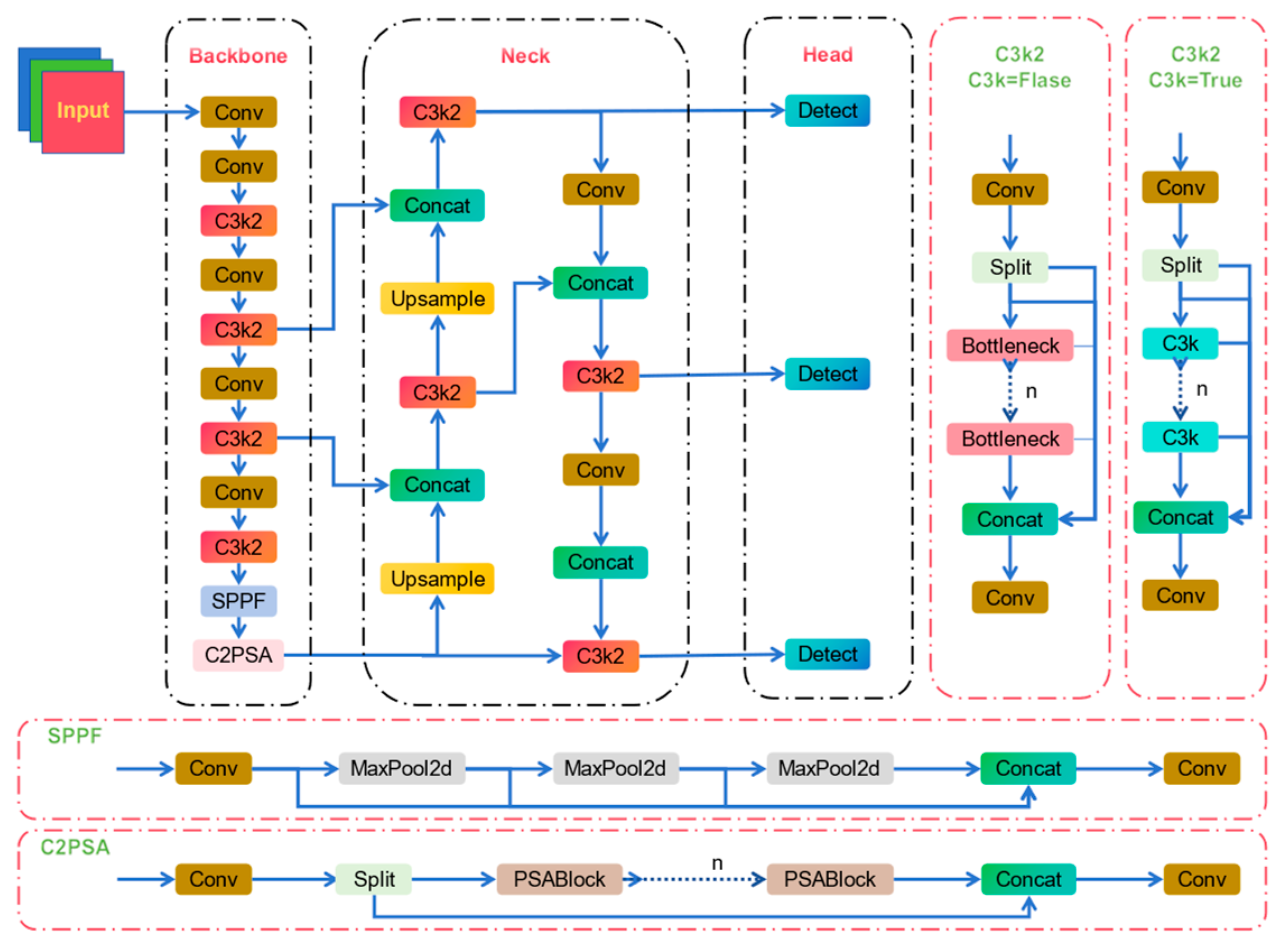
YOLOv11 is a high-performance algorithm officially released by Ultralytics [20]. When compared with the previous YOLO series algorithms, YOLOv11 incorporates several new modules, including C2PSA and C3k2, among others. The enhanced performance of the model is attributable to its augmented flexibility and the capacity for more effective feature extraction. The YOLOv11 model encompasses five distinct network depths: nano (n), small (s), medium (m), large (l), and xlarge (x). The official Ultralytics model on the COCO dataset was utilized to derive the corresponding model training results, as illustrated in

Table 3. Performance comparison of different versions of YOLOv11.

Model	Size	mAP50-95 (%)	CPU ONNX Speed (ms)	T4 TensorRT Speed (ms)	Number of Parameters (M)	FLOPs (B)
YOL011n	640	39.5	56.1 ± 0.8	1.5 ± 0.0	2.6	6.5
YOL011s	640	47.0	90.0 ± 1.2	2.5 ± 0.0	9.4	21.5
YOL011m	640	51.5	183.2 ± 2.0	4.7 ± 0.1	20.1	68.0
YOL011l	640	53.4	238.6 ± 1.4	6.2 ± 0.1	25.3	86.9
YOL011x	640	54.7	462.8 ± 6.7	11.3 ± 0.2	56.9	194.9

.

In the context of agricultural scenarios, the limitations imposed by hardware constraints necessitate the deployment of low-cost embedded devices characterized by constrained computational power, memory, and storage space. The utilization of small models allows for direct execution on these devices, while the deployment of larger models becomes impractical due to the limited computing capacity. Conversely, in scenarios such as automated apple-picking robots or assembly lines for sorting ripe apples, ensuring good real-time performance is imperative. High latency can result in misoperation or missed inspection of the robotic arm. According to the aforementioned rationales, the YOLOv11n model is selected as the foundational model. The model is principally comprised of four components: the image input component (Input); the Backbone, which is responsible for feature extraction; the Neck, which is responsible for feature fusion and enhancement; and the Head, which is responsible for generating the final detection results. The network structure is illustrated in Figure 2.

2.3. Lightweight Apple Maturity Detection Model (BGWL-YOLO)

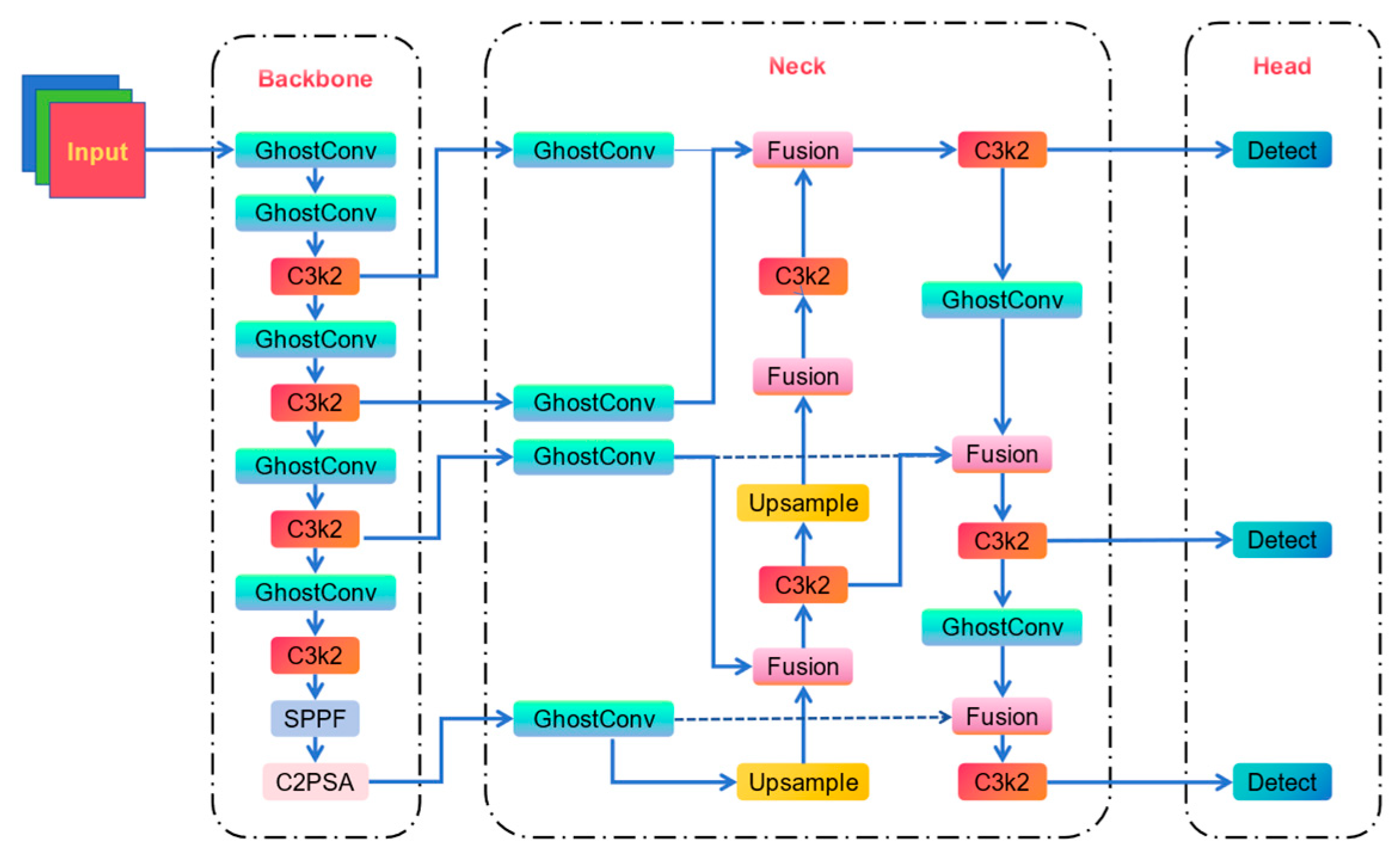
In the context of smart agriculture, where the deployment of apple ripeness detection models on edge devices poses significant challenges, we have devised a lightweight network architecture based on the YOLOv11n model, as depicted in Figure 3.

In this study, we propose a novel approach to enhance the fusion capability of features at different scales of apples. It should be noted that our method incorporates significant improvements from prior works, including BiFPN [21], GhostConv [22], Wise-Inner-MPDIoU [23], and LAMP [24]. Our approach involves replacing the neck structure with a bidirectional weighted feature pyramid network (BiFPN). This modification aims to reduce the number of parameters and the computation volume of the network. Additionally, we introduce GhostConv, a novel convolution alternative, to further reduce the network’s parameters and computation volume. Our approach demonstrates a significant reduction in network complexity, leading to enhanced performance and efficiency in feature fusion tasks. Subsequently, the loss function of the original model is replaced with Wise-Inner-MPDIoU (WIMIoU). This modification has been demonstrated to enhance the training effect of bounding box regression and improve the localization accuracy of the model. Finally, the LAMP pruning process is applied to the improved model. This process serves to further compress the model size and improve the model’s generalization ability.

2.3.1. BiFPN Feature Fusion Network

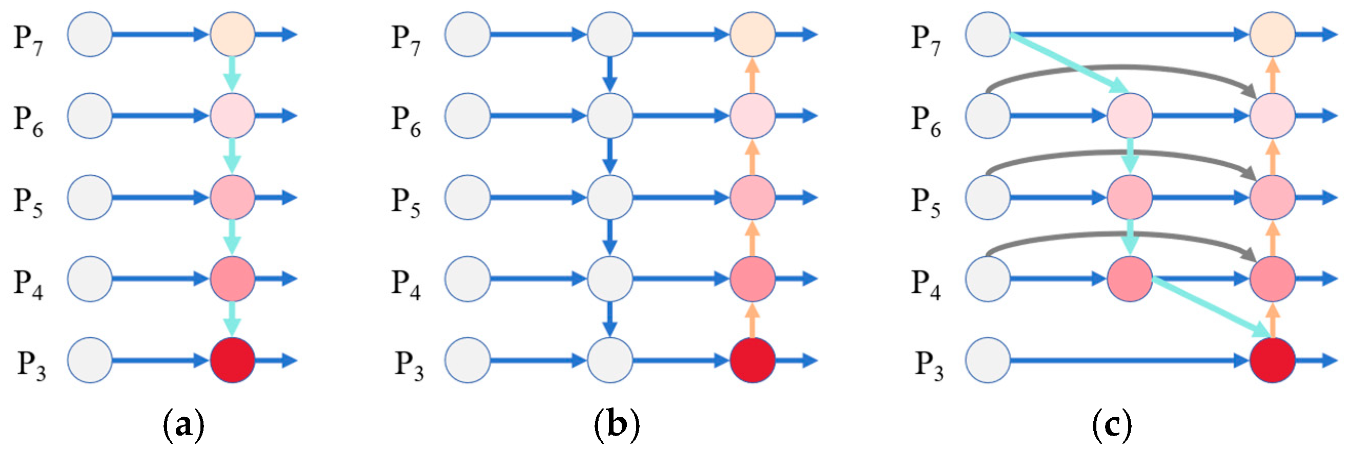
As the depth of the neural network increases, the feature extraction network is capable of capturing higher-order semantic information. However, this process invariably results in a decrease in spatial resolution and a loss of detailed information, which can lead to unsatisfactory model detection [25]. In the event that only detail-rich shallow features are employed for detection, the semantic information is inadequate, leading to deficient model detection. Consequently, to achieve a more comprehensive set of features, it is typically necessary to integrate the feature information of the deep network with that of the shallow network. This integration serves to enhance the detection performance of the model. As illustrated in Figure 4, three classical feature fusion networks are presented.

As illustrated in Figure 4a, the FPN integrates the semantic information of the deep features in a top-down manner with the shallow features through upsampling. However, the transition from shallow to deep features is a complex process, and the information may be lost during the fusion process, leading to inefficiency and the problem of low utilization of the underlying features [26]. As illustrated in Figure 4b, PANet incorporates bottom-up paths derived from the FPN network to establish a two-way fusion, thereby addressing the issue of bottom feature loss in FPN and enhancing the utilization of shallow features for target location. This approach enhances performance and efficiency, though it concomitantly increases model complexity [27]. As illustrated in Figure 4c, BiFPN differs from PANet in several key aspects. Notably, BiFPN eliminates nodes with a single input, introduces jump connections, and repeats the stacking of bi-directional paths as a unit. Additionally, it incorporates weighted fusion, a feature not present in PANet [28]. These enhancements enable BiFPN to assign learnable weights to feature graphs at various scales, mitigating feature loss in deeper networks and fusing features at higher scales. Consequently, this results in a model that exhibits both high accuracy and lightweight characteristics.

2.3.2. GhostConv Module

When the YOLOv11 model is employed to extract features from apple images, a multitude of feature maps exhibiting high similarity are generated during the process. This phenomenon is pivotal to the effective learning of features by the network. However, it concomitantly results in redundant computations during the generation of feature maps by conventional convolution [29]. The GhostConv module, a network module of reduced weight proposed by Huawei Noah’s Ark Lab, aims to generate a low-cost linear transformation to produce redundant feature maps, replacing the large number of repetitive computations in regular convolution. This results in a reduction of the unnecessary computational overhead generated during the convolution process. The working principle of the GhostConv module is shown in Figure 5.

As illustrated in Figure 5, each convolutional layer of the GhostConv module is subdivided into two segments. The initial segment constitutes the conventional convolution, with the number of feature maps being constrained to mitigate excessive computational demands within the network. The second part involves a linear transformation of the regular convolutional feature maps, which results in the generation of additional feature maps. Consequently, the feature maps of the two parts are integrated to generate the output feature maps of the module.

Assuming the existence of input features of size c×h×w for regular convolution, which are processed by n k×k convolution kernels to obtain output features of size n×h’×w’, and the existence of a linear operation convolution kernel d×d with the number of linear transformations of s for phantom convolution, the ratio of computational and parametric quantities of regular convolution and phantom convolution can be expressed as follows, respectively, in Equations (1) and (2):

$$r_F={\displaystyle \frac{n·h^{\prime }·w^{\prime }·c·k·k}{\frac{n}{s}·h^{\prime }·w^{\prime }·c·k·k+\left(s-1\right)·\frac{n}{s}·h^{\prime }·w^{\prime }·d·d}}\approx {\displaystyle \frac{s·c}{s+c-1}}\approx s$$

(1)

$$r_P={\displaystyle \frac{n·c·k·k}{\frac{n}{s}·c·k·k+\left(s-1\right)·\frac{n}{s}·d·d}}\approx {\displaystyle \frac{s·c}{s+c-1}}\approx s$$

(2)

According to Equations (1) and (2), it can be seen that the computational results of both can be approximated as s. If the number of linear transformations is larger, it means that the regular convolution part of the phantom convolution process is smaller. This, in turn, affects the amount of computation and the number of parameters. It is important to note that, without altering the dimensions of the output feature map, the number of parameters and the amount of computation required in the GhostConv module will be reduced in comparison to a standard CNN. Consequently, a more compact apple ripeness detection model can be obtained.

2.3.3. Wise-Inner-MPDIoU (WIMIoU) Loss Function

In the YOLO family of algorithms, the loss function occupies a pivotal role, serving as a metric to quantify the discrepancy between the model’s predicted outcomes and the actual results. In YOLOv11, the loss function employed by the model is the CIoU loss function, which is defined as follows:

$$L_{CIoU}=1-IoU+{\displaystyle \frac{{d_C}^2}{{c_c}^2}}+\propto ·v$$

(3)

where $d_c$ is the centroid distance, $c_c$ is the diagonal distance of the smallest outer rectangle, and $IoU$ is denoted as the intersection and union ratio of the predicted frame to the true frame.

Assuming the existence of a true frame of size W_G×H_G and a predicted frame of size W_P×H_P, the correction factor defining equation is expressed as follows:

$$v={\displaystyle \frac{4(arctan\frac{W_G}{H_G}-arctan\frac{W_P}{H_P})}{{\pi }^2}}$$

(4)

In the event of the intersection and union ratio of the true and predicted frames being IoU, the weighting coefficients are defined as follows:

$$\propto ={\displaystyle \frac{v}{\left(1-IoU\right)+v}}$$

(5)

Assuming that the dimensions of the real frame are 100 × 50 and the dimensions of the predicted frame are 50 × 25, it can be deduced that the aspect ratio of the two is equal at this time. From Equation (3), it can be deduced that the correction factor for both the real frame and the predicted frame is 0. Consequently, from Equation (5), if the center distance of the two frames is 0, it can be concluded that only the IoU term is at work, which results in the slow convergence of the model. To address the aforementioned issues, the MPDIoU loss function is proposed [30], the principle of which is illustrated in Figure 6.

As illustrated in Figure 6, the dimensions of the image are represented by $w_{MPD}$×$h_{MPD}$. Furthermore, MPDIoU takes into account the upper-left corner dot spacing, d1, and the lower-right corner dot spacing, d2, of the real frame and the predicted frame. This is based on IoU, and the MPDIoU loss function is defined by the following equation:

$$L_{MPDIoU}=1-IoU+{\displaystyle \frac{d_1^2}{{w_{MPD}}^2+{h_{MPD}}^2}}+{\displaystyle \frac{d_2^2}{{w_{MPD}}^2-{h_{MPD}}^2}}$$

(6)

As demonstrated in Equation (6), it can be deduced that as the position deviation (d1, d2) increases, the penalty intensity will concomitantly increase. Unless the real box perfectly overlaps with the predicted box, there will be additional penalty intensity to accelerate the convergence speed.

Due to the substantial size of the apple dataset, the presence of low-quality labeled samples is unavoidable, which inevitably affects the detection effect. Therefore, based on MPDIoU, we have optimized MPDIoU by combining the concepts of InnerIoU and WiseIoUv3 to form the Wise-Inner-MPDIoU (WIMIoU) loss function [31,32]. Among these approaches, InnerIoU facilitates the model’s learning process by adjusting the size of the box, thereby optimizing the computation for specific targets. InnerIoU employs a scaling factor ratio to concurrently reduce both the ground truth and the predicted bounding boxes inwards, thereby calculating the IoU within a reduced “inner region”. In the context of small objects, the computation of IoU within this inner region ensures that minor prediction deviations do not result in significant fluctuations in IoU. This approach engenders smoother, more rational gradients, thereby guiding the model in a steady progression towards the correct direction. In instances where target edges are indistinct or ambiguous, the implementation of bounding boxes can facilitate the model’s focus on the most discriminative regions of the target, thereby reducing the impact of background interference on the peripheral pixels. Wise-IoU v3 employs dynamic adjustments to the training process, modulating the learning intensity to mitigate the impact of suboptimal samples on the training of optimal models. The third iteration of Wise-IoU introduces a dynamic gradient gain mechanism, which is predicated on the concept of “outlierness”. In the event of a predicted bounding box exhibiting an IoU that is significantly lower than the ground truth, it is probable that the sample is an outlier, indicating a low-quality or particularly challenging instance. For outliers, the r value decreases. This suggests that the network reduces its learning intensity on these difficult or low-quality samples, thereby preventing the emergence of bias. In the case of regular samples, the r value remains consistent or undergoes an increase. This approach ensures that the network focuses on learning from high-quality, reliable samples. In summary, WIMIoU builds upon MPDIoU by leveraging InnerIoU to provide a more gradient-friendly environment for difficult samples, thereby stabilizing training. Concurrently, the dynamic weighting mechanism from Wise-IoU v3 is employed to automatically mitigate the adverse impact of low-quality samples. This approach has been demonstrated to accelerate convergence, ultimately yielding a detection model with enhanced robustness and superior generalization capabilities. The definition of WIMIoU is provided in Equation (7).

$$L_{WIMIoU}=\mathrm{r}(L_{MPDIoU}+\mathrm{I}\mathrm{o}\mathrm{U}-\mathrm{I}\mathrm{n}\mathrm{n}\mathrm{e}\mathrm{r}\mathrm{I}oU)$$

(7)

In Equation (7), the definitions of InnerIoU and the gradient gain factor r are as follows:

$$\mathrm{I}\mathrm{n}\mathrm{n}\mathrm{e}\mathrm{r}\mathrm{I}\mathrm{o}\mathrm{U}={\displaystyle \frac{\mathrm{i}\mathrm{n}\mathrm{t}\mathrm{e}\mathrm{r}}{union}}$$

(8)

$$inter=\left[\min \left(b_1^g,b_1\right)-\max \left(b_2^g,b_2\right)\right]\left[\min \left(b_3^g,b_3\right)-\max \left(b_4^g,b_4\right)\right]$$

(9)

$$union=(w_{Inner}^g·h_{Inner}^g)(ratio{)}^2+(w_{Inner}^p·h_{Inner}^p\left)\right(ratio{)}^2-inter$$

(10)

$$r={\displaystyle \frac{\beta }{\delta ·{\alpha }^{\beta -\delta }}}$$

(11)

In Equation (8), inter and union are denoted as the intersection area and union area of the real and predicted frames of InnerIoU, respectively. In Equation (9), $b_1^g$~$b_4^g$ are the boundary coordinates of the real frame, and $b_1$~$b_4$ are the boundary coordinates of the predicted frame. In Equation (10), ratio, $w_{Inner}^g$, $h_{Inner}^g$, $w_{Inner}^p$, and $h_{Inner}^p$ represent the scaling factor of InnerIoU, the width and height of the real frame, and the width and height of the prediction frame, respectively. In Equation (11), β and δ are denoted as the hyperparameters of the gradient gain factor r of WiseIoU.

2.3.4. Experiment of LAMP Pruning

In the field of machine learning, “model pruning” refers to the process of reducing the size and computational complexity of a model by removing some weights from the neural network. This technique has been demonstrated to be particularly effective for neural networks when deployed on resource-constrained devices, such as mobile devices and embedded systems.

The present study employs Layer Adaptive Magnitude-Based Pruning (LAMP) to address the challenge of selecting hierarchical sparsity [33]. LAMP quantifies model distortion by computing a score, and all channel connections with LAMP scores lower than the target weights are pruned. Assuming a feedforward neural network with depth g, the weight tensor W(1)...W(g) is expanded into a one-dimensional vector. The inequality W[x] ≤ W[y] holds whenever x < y. The LAMP score for the xth index of the weight tensor W is computed as follows:

$$score\left(x;W\right):={\displaystyle \frac{{\left(W\left[x\right]\right)}^2}{{\Sigma }_{y\ge x}(W\left[y\right]{)}^2}}$$

(12)

Among them, the larger weighted $W\left[x\right]$ will receive a higher score and is more likely to be retained in the pruning process. Therefore, the LAMP score calculation does not require the setting of other hyperparameters, and the important weights can be automatically retained only by the basic tensor operation. In the network structure of YOLO, there are different levels of important feature weights. This adaptive pruning property of LAMP can find the appropriate pruning intensity for each layer of the model’s structure, so as to retain the key important weights.

2.4. Experimental Environment

The experimental hardware environment consists of the following components: the processor is an AMD Ryzen 5 6600H with Radeon Graphics, operating at 3.30 GHz; the graphics card is an NVIDIA GeForce RTX 3050 Laptop GPU with 4 GB of memory; and the RAM is 16.0 GB. The experimental software environment is as follows: the Pytorch deep learning framework is utilized, with the operating system being Windows 11 Professional. The Python version is 3.9.21, and the CUDA version is 12.5. The network hyperparameters employed during the training of the YOLOv11n model are shown in

Table 4. Table of network hyperparameters.

Name of Hyperparameter	Parameter Value
Image input size	640 × 640
Training batch	200
Batch size	16
Number of work processes	1
Optimizer	SGD
Initial learning rate	0.01
Learning rate attenuation strategy	cos

below.

2.5. Evaluation Indicators

The classical performance evaluation metrics of target detection models include recall (R), precision (P), accuracy of individual categories (AP), and mean average precision (mAP). Furthermore, the amount of computation (FLOPs), the number of parameters (Params), the frame rate (FPS), and the model size are introduced as the evaluation indices of the lightweighting effect of the apple maturity detection model. The calculation formula is as follows:

$$P={\displaystyle \frac{TP}{\left(TP+FP\right)}}\times 100\%$$

(13)

$$R={\displaystyle \frac{TP}{\left(TP+FN\right)}}\times 100\%$$

(14)

$$mAP={\displaystyle \frac{{\sum }_{j=1}^{k}A{P}_j}{k}}$$

(15)

$$FPS={\displaystyle \frac{frame\_number}{time}}$$

(16)

Among them, for Equations (13) and (14), TP signifies the number of positive sample instances that have been correctly identified by the model, FP denotes the number of negative sample instances that have been erroneously classified as positive classes, and FN represents the number of missed instances that are actually positive classes but have not been detected. For Equation (15), for the purpose of measuring the comprehensive performance of the model, the arithmetic mean of the AP values of the model across all categories is denoted as mAP. The number of categories is represented by k, and the indices of different categories are represented by j. As illustrated in Equation (16), the variable frame_number denotes the number of image frames, while time signifies the duration required for the model to detect all images.

3. Experiments and Results Analysis

3.1. Visualization of the Model Training Process

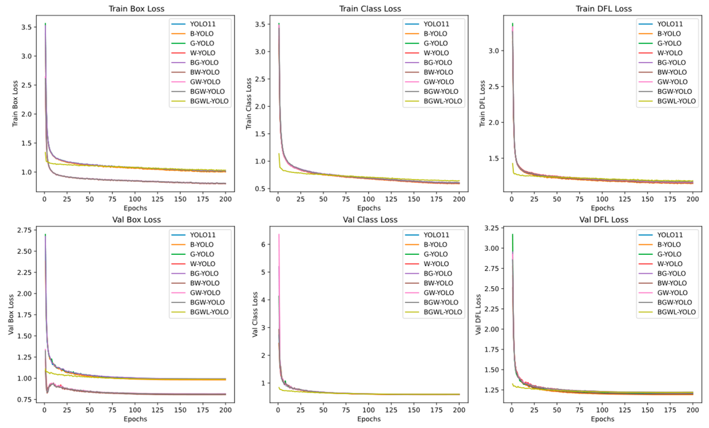
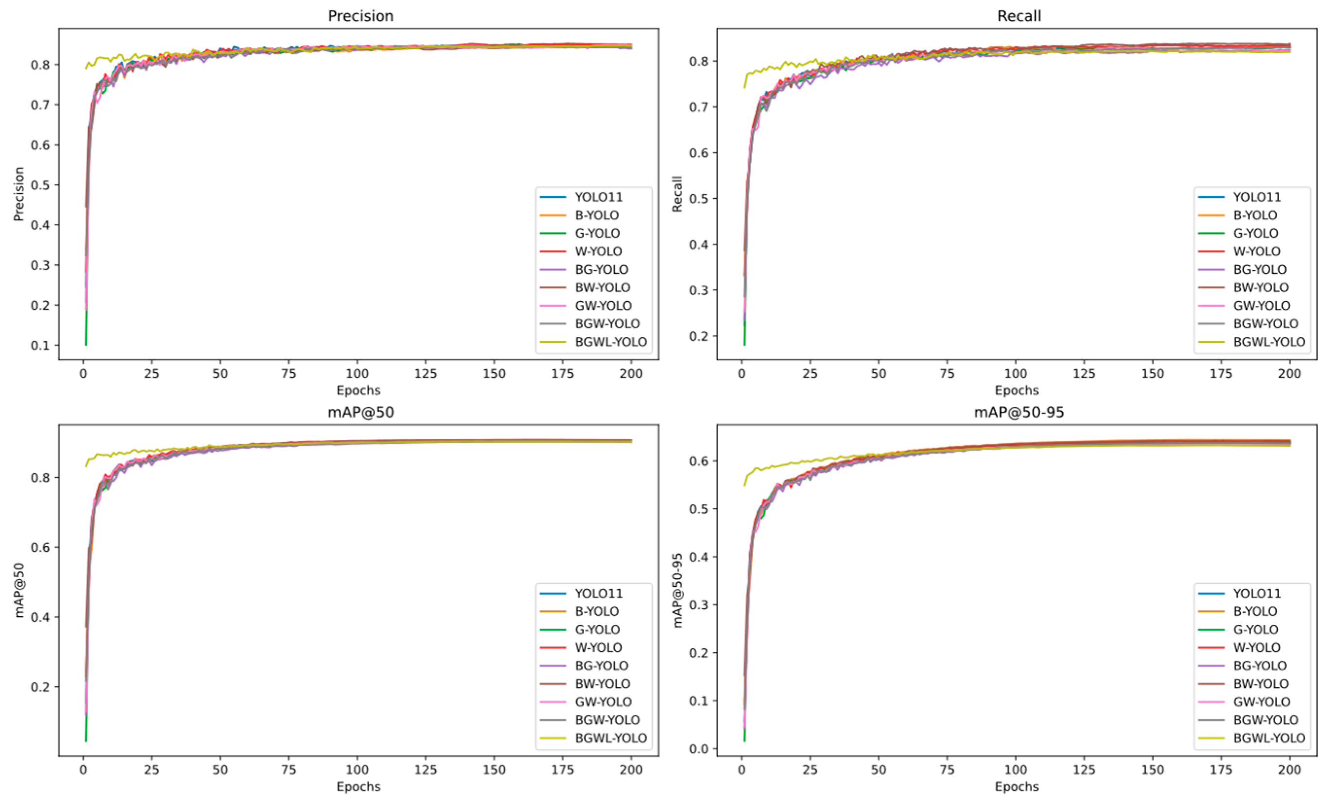
In this present study, we introduce four key technological improvements in a targeted manner. These improvements are based on the YOLOv11 framework. The following four steps are taken in order to successfully implement the proposed methodology: (1) the adoption of the GhostConv lightweight convolution module (G module); (2) the integration of the BiFPN bi-directional feature pyramid network (B module); (3) the introduction of the WIMIoU weighted intersection and merger ratio loss function (W module); and (4) the design of the LAMP dynamic label assignment strategy (L module). In order to systematically assess the convergence and stability of the model training, the optimization path of the model parameters and the evolution of the generalization ability during the training process are visualized by means of the change curve of the loss function, demonstrated in Figure 7, and the change curve of the mAP and other indicators presented in Figure 8.

As illustrated in Figure 7 and Figure 8, the prefix “YOLO” denotes the processing means, with “GB-YOLO” representing the incorporation of GhostConv and BiFPN modules based on YOLOv11. As demonstrated by the training results presented in Figure 7, the loss curves exhibit a rapid decrease from high to low values during the initial 25 iterations, suggesting that the model can rapidly converge on a solution for the apple ripeness detection task. The validation set exhibited a similar trend to the training set and ultimately stabilized at a low level, indicating that there was no evident overfitting phenomenon. As demonstrated in Figure 8, the training outcomes exhibit remarkable stability in the accuracy metrics of the models, irrespective of the employed methodology for processing the dataset. This stability is evident from the initial 50 rounds, particularly in the mAP50 metric. As demonstrated in Figure 8, the value of mAP50 is considerably higher than that of mAP50-95, suggesting that the models are effective in identifying targets but demonstrate a deficiency in target localization. This deficiency can be attributed to the high complexity of the samples in our dataset, which results in an inadequate localization ability.

3.2. Ablation Experiments

In order to verify the effectiveness of the improvement, the YOLOv11n baseline model is utilized, to which various modules of GhostConv, BiFPN, and WIMIoU are added to explore their effects on the network. A total of eight experiments were designed, denoted by A to H. As illustrated in

Table 5. Results of the ablation experiments.

Model	GhostConv	BiFPN	WIMIoU	mAP50 (%)	Number of Parameters	GFLOPs	Model Size (MB)	FPS
A				89.8	2,582,542	6.3	5.21	232.6
B	√			89.6	2,256,846	5.5	4.60	222.5
C		√		90.2	1,923,018	6.3	3.98	207.0
D			√	90.0	2,582,542	6.3	5.21	233.8
E	√	√		89.8	1,620,202	5.3	3.43	197.9
F	√		√	89.9	2,256,846	5.5	4.60	222.5
G		√	√	90.1	1,923,018	6.3	3.98	208.8
H	√	√	√	90.0	1,620,202	5.3	3.43	197.4

, the results of the ablation experiments are presented. In this table, “√” denotes the utilization of the module.

A comparative analysis of the four sets of experiments, A, B, C, and D, reveals that the incorporation of the GhostConv module alone on top of YOLOv11n leads to a reduction in computation, number of parameters, and model size by 12.7%, 12.6%, and 11.7%, respectively. Additionally, it causes a decline in mAP50 and FPS by 0.2% and 4.3%, respectively. The incorporation of a distinct BiFPN module on top of YOLOv11n results in a 25.5% and 23.6% reduction in model parameters and size, respectively, while concurrently enhancing mAP50 by 0.4%. However, this approach concomitantly leads to an 11.0% decrease in FPS. The introduction of a discrete WIMIoU module based on YOLOv11n does not result in alterations to the computational process, the quantity of parameters, or the model’s dimensionality. However, it has been observed to enhance mAP50 by 0.2% and FPS by 0.5%. A comparative analysis of the four sets of experiments in E, F, G, and H reveals that the removal of one of the three improvements individually leads to an augmentation in the model size or a reduction in the accuracy. This is evidenced by the increase in model size from 0.55MB to 1.17MB when GhostConv or BiFPN is removed individually, and the removal of the WIMIoU loss function results in a decline in accuracy of 0.2%. In summary, the proposed improvement strategy results in a model of reduced size, but there is also a decrease in FPS. A pruning strategy will be employed to further improve FPS.

3.3. Pruning Experiment

In order to facilitate the embedding of the model on edge devices with reduced resource allocation, the LAMP pruning technique is introduced to prune the GBW-YOLO model. In light of the constrained computational resources available, the number of batches in the experimental environment is reduced to eight, while all other conditions remain constant. The pruning rate is defined as the ratio of computation before and after model pruning. Six sets of pruning experiments with LAMP at pruning rates of 1.5, 2, 2.5, 3, 3.5, and 4.0 were designed, and the results are shown in

Table 6. Performance comparison results of GBW-YOLO under different pruning rates.

Pruning Rate	mAP50 (%)	Number of Parameters	GFLOPs	Model Size (MB)	FPS
1.5	90.3	757,846	3.5	1.82	222.7
2.0	90.1	490,870	2.6	1.31	246.1
2.5	89.7	378,831	2.1	1.08	258.9
3.0	89.4	297,752	1.7	1.41	283.7
3.5	88.7	250,856	1.5	0.86	294.7
4.0	88.7	223,726	1.3	0.81	311.2

below.

As illustrated in Table 6, when the pruning rate is configured to rise in a gradual manner, the mAP50, the number of parameters, the volume of computation, and the model’s dimensions undergo a concurrent decline, while the FPS undergoes a steady rise. At a pruning rate of 2.5, the mAP50 is only 89.7%, which is lower than the 89.8% of the original YOLOv11n model. The objective of our work is to further reduce the model size without compromising the performance of the original model, which does not meet our expectations at a pruning rate of more than 2.5. Furthermore, at a pruning rate of 1.5, the FPS is lower than that of the original model at GPU acceleration of 232.6. It is evident that in order to efficiently reconcile between the model lightweighting requirements and the detection performance, it is necessary to finalize the LAMP algorithm configuration with a pruning rate of 2.0.

In order to ascertain the most efficacious pruning method, a comparative analysis was conducted on the effects of Random, L1, and Group_Norm on the mAP50 and lightweighting effects on the apple ripeness detection task. Random pruning involves the random selection of weights, L1 pruning involves the removal of filters exhibiting minimal contribution to the convolutional neural network, and Group_Norm pruning involves dependency graph-centred pruning. The comparative results of each pruning method are presented in

Table 7. Comparison experiment of different pruning algorithms.

Pruning Method	mAP50 (%)	Number of Parameters	(GFLOPs)	Model Size (MB)	FPS
BGW-YOLO	90.0	2,343,604	5.5	4.79	197.4
Random	80.7	1,086,630	2.6	2.45	285.0
L1	88.4	1,440,468	2.6	1.86	249.5
Group_Norm	87.7	1,170,328	2.6	2.61	235.1
LAMP	90.1	490,870	2.6	1.31	246.1

.

As demonstrated in Table 7, there are significant differences in the effects of different pruning methods on model performance, under the condition of a pruning rate of 2.0. The random pruning strategy has the most serious decrease in mAP50, with a significant drop of 9.3%. Although effective in improving the FPS, L1 pruning has a loss of 1.6% of the mAP50. Group_Norm is not as effective as L1 pruning in all aspects of the metrics. In the context of LAMP pruning, the superfluous weights of the model are efficiently eliminated, leading to an unanticipated augmentation of 0.1% in mAP50. Concurrently, it is the most efficacious in compressing the model, with a weight file of merely 1.31MB, which is a mere 1.4% difference from the FPS of L1 pruning. In summary, following a comprehensive evaluation of the detection accuracy and lightweighting effect, it is evident that LAMP demonstrates the optimal pruning effect in comparison to all other methods.

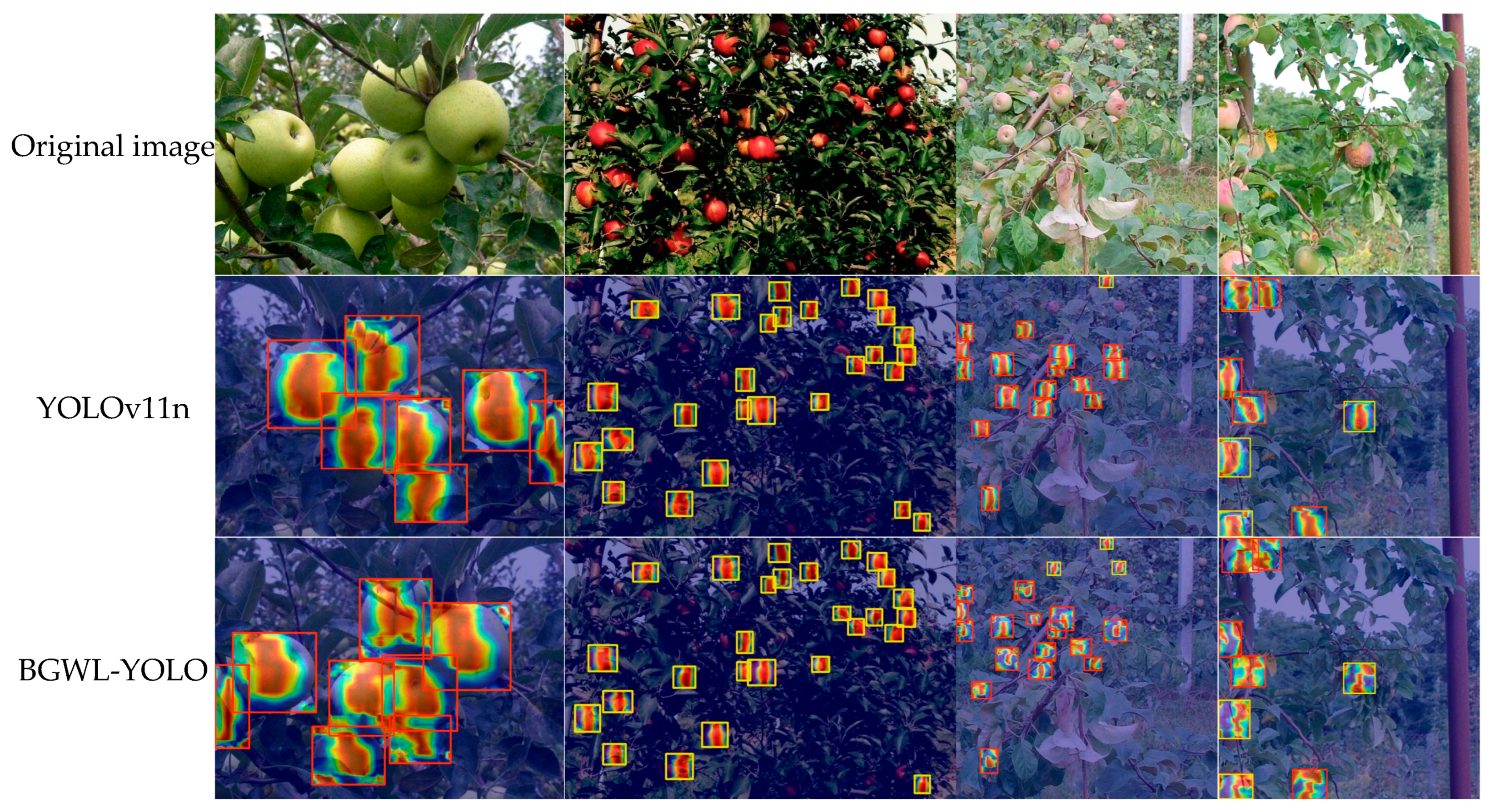
The application of a heat map serves to illustrate the extent to which the model focuses on distinct regions of the apple image, as demonstrated by the color gradient. In order to compare the difference between the pruned model and the original model in terms of the attention paid to the apple image, a KPCA-CAM heat map was drawn, as shown in Figure 9.

As illustrated in Figure 9, the utilization of red signifies a high-attention area, whereas blue denotes a low-attention area. It has been demonstrated that BGWL-YOLO exhibits a high degree of sensitivity to occluded targets; for instance, in the first image, BGWL-YOLO identifies one additional low-maturity apple compared to the original model. Furthermore, BGWL-YOLO demonstrates proficiency in detecting small-target apples, as evidenced in the second and third images. However, it was also found that the sensitivity of BGWL-YOLO to apple fruits is less concentrated and more scattered than in the original model. This finding indicates that BGWL-YOLO is not interested in the characteristics of the apples themselves, but more in the dependency relationship between the fruits and the surrounding environment.

3.4. Comparative Experiments of Different Models

Following the application of the LAMP pruning algorithm to optimise the BGW-YOLO model, the optimised model was named BGWL-YOLO. In order to evaluate the model’s performance in detecting the level of ripeness in apples, five models were selected for comparison and analysis under identical experimental conditions. These models included YOLOv3n, YOLOv5n, YOLOv8n, YOLOv9t, and YOLOv10n. The experimental setup was designed to ensure that the FPS data was collected only when the CPU was operational. This approach was adopted to facilitate a more comprehensive and objective evaluation of the model’s lightweight performance. The specific comparison results are presented in

Table 8. Comparison results of different models.

Model	mAP50 (%)	Number OF Parameters	GFLOPs	Model Size (MB)	FPS1	FPS2
YOLOv3n	88.3	12,128,692	18.9	23.20	173.7	11.9
YOLOv5n	89.2	2,503,334	7.1	5.02	242.8	24.5
YOLOv8n	89.5	3,006,038	8.1	5.95	240.0	22.6
YOLOv9t	89.9	1,971,174	7.6	4.41	178.0	19.7
YOLOv10n	90.2	2,265,558	6.5	5.48	224.7	22.6
YOLOv11n	89.8	2,582,542	6.3	5.21	232.6	22.9
BGWL-YOLO	90.1	490,870	2.6	1.31	246.1	30.4

Note: FPS1 represents the frame rate under GPU acceleration, and FPS2 represents the frame rate under CPU operation.

.

As demonstrated in Table 8, the proposed model, BGWL-YOLO, exhibits an average accuracy of 90.1%, the number of parameters of 490,870, a computational volume of 2.6 GFLOPs, a model size of 1.31 MB, and an FPS of 246.1 under GPU acceleration, and an FPS of 30.4 for CPU-only operation. It is evident from Table 8 that the proposed model performs optimally across all models, particularly in the reference model size, which is considerably lower than that of the other models.

For the original model YOLOv11n, the mAP50 score of our model increases by 0.3%, the number of parameters decreases by 81.0%, the amount of computation decreases by 58.7%, the model size decreases by 3.90 MB, and FPS1 improves by 5.8% and FPS2 improves by 32.8%. Compared to YOLOv10n, our model exhibits a 0.1% decrease in mAP50 yet concomitantly experiences a 78.3% reduction in the number of parameters, a 60.0% decrease in computation, a 4.17 MB decrease in model size, a 9.5% increase in FPS1, and a 34.5% increase in FPS2. For the other models, improvements by BGWL-YOLO were substantial for most criteria. In summary, the proposed BGWL-YOLO model demonstrates superior apple maturity detection accuracy, while also exhibiting excellent lightweight performance and being well-suited for deployment on resource-constrained edge devices.

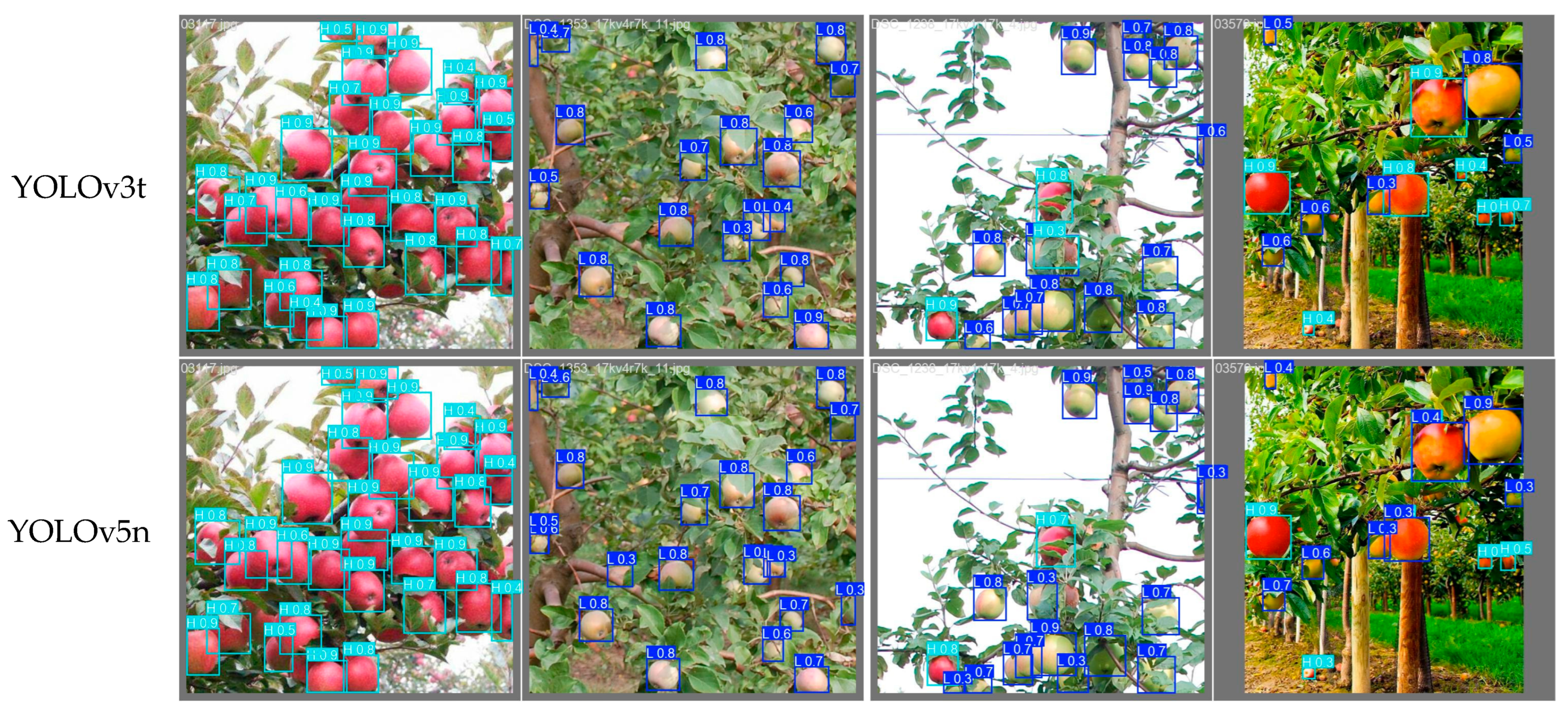
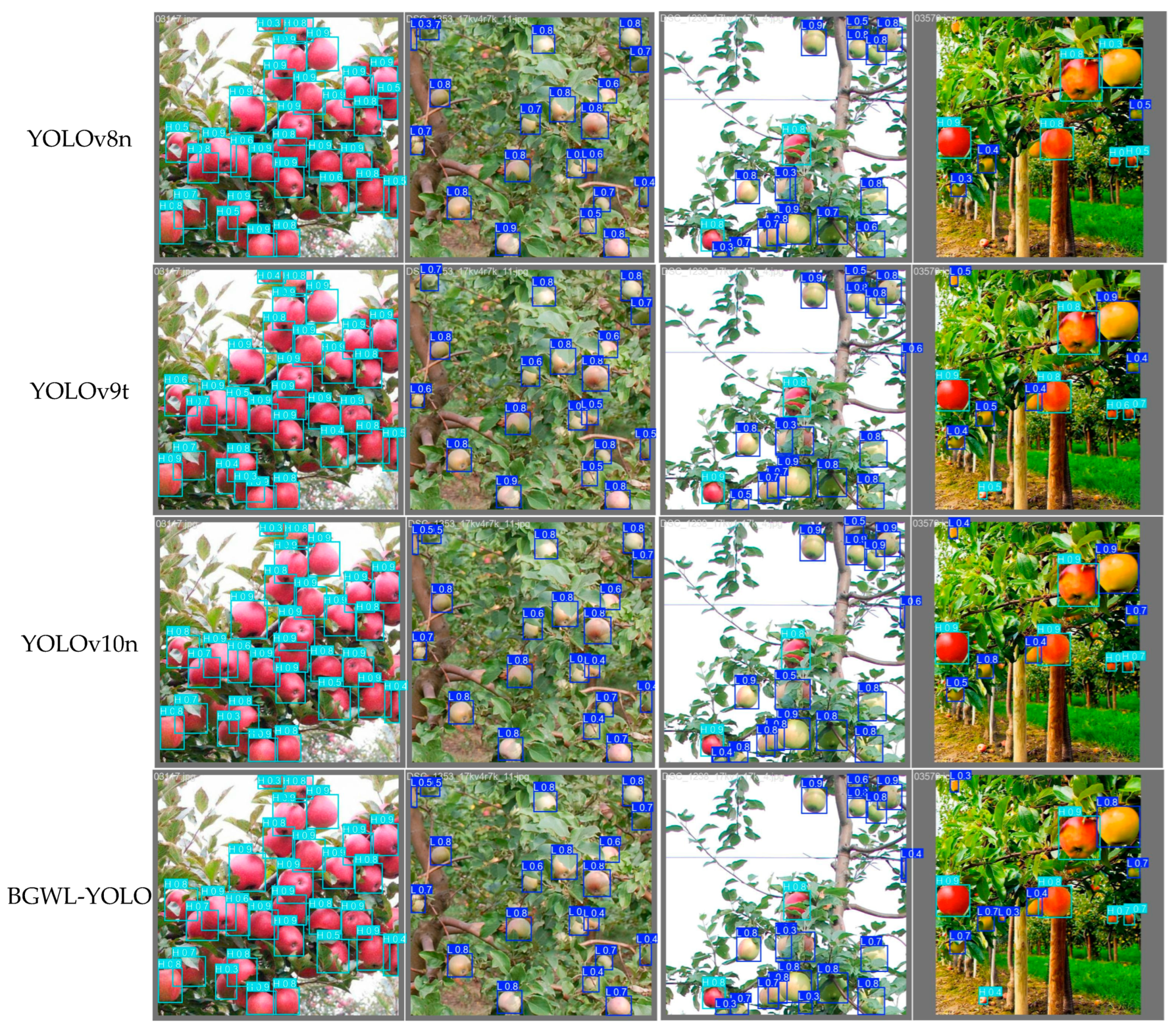
As demonstrated in the preceding analysis, the mean average accuracy of all models ranges from 88.3% to 90.1%, with no discernible discrepancy. To substantiate these findings, an evaluation was conducted on the test set, and the test results are presented in Figure 10.

As demonstrated in Figure 10, it is evident that all models demonstrate a high degree of accuracy in identifying the majority of fruits. However, variations in the extent of missed detections were also observed. In the initial sample image, all models exhibited the capacity to detect the red apple, which was obscured by leaves in the lower right corner. With regard to the second sample image, with the exception of YOLOv9t, which was able to accurately identify the object, all other models exhibited false positives. For instance, in the top-right corner of the second image, the YOLOv5n model erroneously identified the tree trunk as an apple, leading to the incorrect classification of a single apple as two apples on the far right. This resulted in a false positive rate of 9.1%. Furthermore, the YOLOv3t model exhibited false negative detection, as evidenced by the apple located at the lower-right corner being overlooked. As demonstrated in the third sample image, YOLOv3t produced a false positive, whereas BGWL-YOLO accurately identified it. In the case of the red apples located in the middle-lower section of the image, alternative models were unable to detect them. In the fourth sample image, all models exhibited false detections on the apples in the lower left corner, with the exception of YOLOv10n, which demonstrated false negative detection capability. In summary, there is no obvious discrepancy between the detection results of all models; however, our model has a lightweight advantage over the other models.

4. Discussion

The integration of the phantom convolution module, BiPFN feature fusion network, WIMIoU loss function, and LAMP pruning within the YOLOv11 model was met with noteworthy outcomes. The experimental results demonstrated a substantial reduction in model parameters by 81.0%, accompanied by a significant decrease in computation complexity by 58.7%, in comparison to the original model. Concurrently, there was an augmentation in mAP50 by 0.3%. This integration approach signifies a substantial reduction in model complexity, while concurrently ensuring the preservation of the model’s detection accuracy. The lightweight design is of particular significance for the actual deployment of the model, especially in scenarios where resources are limited and multiple models must operate in conjunction.

5. Conclusions

In this study, a lightweight target detection model, named BGWL-YOLO, is proposed for detecting the ripeness condition of apples. This addresses the difficulty of deploying larger models for small devices, with the following main contributions:

(1) A dataset comprising 10,320 images of apples has been constructed, and a lightweight model, BGW-YOLO, has been designed to greatly reduce the number of parameters and computations. The BiFPN feature fusion network is first incorporated into the neck of the model, and then the Conv module of the model is replaced with the GhostConv module, followed by replacing the CIoU of the original model with the Wise-Inner-MPDIoU loss function.

(2) In this study, the LAMP pruning method is applied to the BGW-YOLO model, and the optimal pruning rate is determined. This approach effectively reduces the redundancy of the model without compromising its accuracy, while concurrently enhancing its inference speed.

(3) The BGW-YOLO model demonstrates optimal comprehensive performance in comparison with other YOLO models. In comparison with the baseline model YOLOv11n, the mean average accuracy has been enhanced by 0.3%, the number of parameters and computation have been reduced by 65.3% and 57.1%, respectively, the FPS has been improved by 5.8% on GPU and 32.8% on CPU, and the size of the weight file is only 25.2% of the original model.

The primary focus of our work is the provision of lightweight technical support for the deployment of multiple models on edge devices. In the research, the following aspects were explored: the introduction of knowledge distillation, the optimization of model structure, and multimodality to further improve detection accuracy, and the promotion of the development of smart agriculture.

References

1. Zhao, J.; Lipani, A.; Schillaci, C. Fallen apple detection as an auxiliary task: Boosting robotic apple detection performance through multi-task learning. Microelectron. J. 2024, 8, 100436. [Google Scholar] [CrossRef]
2. Xu, W.; Wang, R. ALAD-YOLO: An lightweight and accurate detector for apple leaf diseases. Front. Plant Sci. 2023, 14, 1204569. [Google Scholar]
3. Chu, P.; Li, Z.; Zhang, K.; Chen, D.; Lammers, K.; Lu, R. O2RNet: Occluder-occludee relational network for robust apple detection in clustered orchard environments. Smart Agric. Technol. 2023, 5, 100284. [Google Scholar] [CrossRef]
4. Li, N.; Wu, Y.; Jiang, Z.; Mou, Y.; Ji, X.; Huo, H.; Dong, X. Efficient Identification and Classification of Pear Varieties Based on Leaf Appearance with YOLOv10 Model. Horticulturae 2025, 11, 489. [Google Scholar] [CrossRef]
5. Hou, J.; Che, Y.; Fang, Y.; Bai, H.; Sun, L. Early bruise detection in apple based on an improved faster RCNN model. Horticulturae 2024, 10, 100. [Google Scholar] [CrossRef]
6. Badgujar, C.M.; Poulose, A.; Gan, H. Agricultural object detection with You Only Look Once (YOLO) Algorithm: A bibliometric and systematic literature review. Comput. Electron. Agric. 2024, 223, 109090. [Google Scholar] [CrossRef]
7. Barhate, D.; Pathak, S.; Singh, B.K.; Jain, A.; Dubey, A.K. A systematic review of machine learning and deep learning approaches in plant species detection. Smart Agric. Technol. 2024, 9, 100605. [Google Scholar] [CrossRef]
8. Liao, H.; Wang, G.; Jin, S.; Liu, Y.; Sun, W.; Yang, S.; Wang, L. HCRP-YOLO: A lightweight algorithm for potato defect detection. Smart Agric. Technol. 2025, 10, 100849. [Google Scholar] [CrossRef]
9. Luo, Y.; Lin, K.; Xiao, Z.; Lv, E.; Wei, X.; Li, B.; Zeng, Z. PBR-YOLO: A lightweight piglet multi-behavior recognition algorithm based on improved yolov8. Smart Agric. Technol. 2025, 10, 100785. [Google Scholar] [CrossRef]
10. Zheng, Z.; Chen, L.; Wei, L.; Huang, W.; Du, D.; Qin, G.; Wang, S. An efficient and lightweight banana detection and localization system based on deep CNNs for agricultural robots. Smart Agric. Technol. 2024, 9, 100550. [Google Scholar] [CrossRef]
11. Tang, B.; Zhou, J.; Li, X.; Pan, Y.; Lu, Y.; Liu, C.; Gu, X. Detecting tasseling rate of breeding maize using UAV-based RGB images and STB-YOLO model. Smart Agric. Technol. 2025, 11, 100893. [Google Scholar] [CrossRef]
12. Moreira, G.; dos Santos, F.N.; Cunha, M. Grapevine inflorescence segmentation and flower estimation based on Computer Vision techniques for early yield assessment. Smart Agric. Technol. 2025, 10, 100690. [Google Scholar] [CrossRef]
13. Wang, C.; Han, Q.; Li, J.; Li, C.; Zou, X. YOLO-BLBE: A novel model for identifying blueberry fruits with different maturities using the I-MSRCR method. Agronomy 2024, 14, 658. [Google Scholar] [CrossRef]
14. Ling, C.; Zhang, Q.; Zhang, M.; Gao, C. Research on adaptive object detection via improved HSA-YOLOv5 for raspberry maturity detection. IET Image Process. 2024, 18, 4898–4912. [Google Scholar] [CrossRef]
15. Badeka, E.; Karapatzak, E.; Karampatea, A.; Bouloumpasi, E.; Kalathas, I.; Lytridis, C.; Kaburlasos, V.G. A deep learning approach for precision viticulture, assessing grape maturity via YOLOv7. Sensors 2023, 23, 8126. [Google Scholar] [CrossRef]
16. Xu, D.; Ren, R.; Zhao, H.; Zhang, S. Intelligent detection of muskmelon ripeness in greenhouse environment based on YOLO-RFEW. Agronomy 2024, 14, 1091. [Google Scholar] [CrossRef]
17. Sun, H.; Ren, R.; Zhang, S.; Tan, C.; Jing, J. Maturity detection of ‘Huping’ jujube fruits in natural environment using YOLO-FHLD. Smart Agric. Technol. 2024, 9, 100670. [Google Scholar] [CrossRef]
18. Jing, J.; Zhang, S.; Sun, H.; Ren, R.; Cui, T. Detection of maturity of “Okubo” peach fruits based on inverted residual mobile block and asymptotic feature pyramid network. J. Food Meas. Charact. 2025, 19, 682–695. [Google Scholar] [CrossRef]
19. Wei, J.; Ni, L.; Luo, L.; Chen, M.; You, M.; Sun, Y.; Hu, T. GFS-YOLO11: A maturity detection model for multi-variety tomato. Agronomy 2024, 14, 2644. [Google Scholar] [CrossRef]
20. Sapkota, R.; Meng, Z.; Karkee, M. Synthetic meets authentic: Leveraging llm generated datasets for yolo11 and yolov10-based apple detection through machine vision sensors. Smart Agric. Technol. 2024, 9, 100614. [Google Scholar] [CrossRef]
21. Touko Mbouembe, P.L.; Liu, G.; Park, S.; Kim, J.H. Accurate and fast detection of tomatoes based on improved YOLOv5s in natural environments. Front. Plant Sci. 2024, 14, 1292766. [Google Scholar] [CrossRef]
22. Thakuria, A.; Erkinbaev, C. Improving the network architecture of YOLOv7 to achieve real-time grading of canola based on kernel health. Smart Agric. Technol. 2023, 5, 100300. [Google Scholar] [CrossRef]
23. Huang, Y.; Ouyang, H.; Miao, X. LSOD-YOLOv8: Enhancing YOLOv8n with New Detection Head and Lightweight Module for Efficient Cigarette Detection. Appl. Sci. 2025, 15, 3961. [Google Scholar] [CrossRef]
24. Sun, W.; Meng, N.; Chen, L.; Yang, S.; Li, Y.; Tian, S. CTL-YOLO: A Surface Defect Detection Algorithm for Lightweight Hot-Rolled Strip Steel Under Complex Backgrounds. Machines 2025, 13, 301. [Google Scholar] [CrossRef]
25. Seol, S.; Ahn, J.; Lee, H.; Kim, Y.; Chung, J. SSP based underwater CIR estimation with S-BiFPN. ICT Express 2022, 8, 44–49. [Google Scholar] [CrossRef]
26. Rajeev, P.A.; Dharewa, V.; Lakshmi, D.; Vishnuvarthanan, G.; Giri, J.; Sathish, T.; Alrashoud, M. Advancing e-waste classification with customizable YOLO based deep learning models. Sci. Rep. 2025, 15, 18151. [Google Scholar] [CrossRef] [PubMed]
27. Chakrabarty, S.; Shashank, P.R.; Deb, C.K.; Haque, M.A.; Thakur, P.; Kamil, D.; Dhillon, M.K. Deep learning-based accurate detection of insects and damage in cruciferous crops using YOLOv5. Smart Agric. Technol. 2024, 9, 100663. [Google Scholar] [CrossRef]
28. Saraei, M.; Lalinia, M.; Lee, E.J. Deep Learning-Based Medical Object Detection: A Survey. IEEE Access 2025, 13, 53019–53038. [Google Scholar] [CrossRef]
29. Yaamini, H.G.; Swathi, K.J.; Manohar, N.; Kumar, A. Lane and Traffic Sign Detection for Autonomous Vehicles: Addressing Challenges on Indian Road Conditions. MethodsX 2025, 14, 103178. [Google Scholar] [CrossRef]
30. Lv, Q.; Sun, F.; Bian, Y.; Wu, H.; Li, X.; Li, X.; Zhou, J. A Lightweight Citrus Object Detection Method in Complex Environments. Agriculture 2025, 15, 1046. [Google Scholar] [CrossRef]
31. Jiang, X.; Tang, D.; Xu, W.; Zhang, Y.; Lin, Y. Swimming-YOLO: A drowning detection method in multi-swimming scenarios based on improved YOLO algorithm. Signal Image Video Process. 2025, 19, 161. [Google Scholar] [CrossRef]
32. Shen, Q.; Li, Y.; Zhang, Y.; Zhang, L.; Liu, S.; Wu, J. CSW-YOLO: A traffic sign small target detection algorithm based on YOLOv8. PLoS ONE 2025, 20, e0315334. [Google Scholar] [CrossRef] [PubMed]
33. Dai, S.; Bai, T.; Zhao, Y. Keypoint Detection and 3D Localization Method for Ridge-Cultivated Strawberry Harvesting Robots. Agriculture 2025, 15, 372. [Google Scholar] [CrossRef]
Figure 1. Sample plot of the apple datasets: (a) Dataset A sample; (b) Dataset B sample; (c) Dataset C sample; (d) Dataset D sample.
Horticulturae 11 01068 g001
Figure 2. YOLOv11 network architecture.
Horticulturae 11 01068 g002
Figure 3. Lightweight YOLOv11 network structure.
Horticulturae 11 01068 g003
Figure 4. Structure diagram of three main feature fusion networks: (a) FPN; (b) PANet; (c) BiFPN.
Horticulturae 11 01068 g004
Figure 5. Workflow diagram of the GhostConv module.
Horticulturae 11 01068 g005
Figure 6. Schematic diagram of MPDIoU.
Horticulturae 11 01068 g006
Figure 7. Diagram of model loss variation.
Horticulturae 11 01068 g007
Figure 8. Diagram of model accuracy variation.
Horticulturae 11 01068 g008
Figure 9. Heat maps of KPCA-CAM before and after improvement.
Horticulturae 11 01068 g009
Figure 10. Detection effects of different models on the test set.
Horticulturae 11 01068 g010aHorticulturae 11 01068 g010b