Article

Optimizing Plant Production Through Drone-Based Remote Sensing and Label-Free Instance Segmentation for Individual Plant Phenotyping

1
Plant Sciences Unit, Flanders Research Institute for Agriculture, Fisheries and Food (ILVO), Caritasstraat 39, 9090 Merelbeke-Melle, Belgium
2
Department of Data Analysis and Mathematical Modelling, Ghent University, Coupure Links 653, 9000 Ghent, Belgium
*
Author to whom correspondence should be addressed.
Horticulturae 2025, 11(9), 1043; https://doi.org/10.3390/horticulturae11091043
Submission received: 4 July 2025 / Revised: 7 August 2025 / Accepted: 15 August 2025 / Published: 2 September 2025
(This article belongs to the Special Issue Emerging Technologies in Smart Agriculture)

Abstract

A crucial initial step for the automatic extraction of plant traits from imagery is the segmentation of individual plants. This is typically performed using supervised deep learning (DL) models, which require the creation of an annotated dataset for training, a time-consuming and labor-intensive process. In addition, the models are often only applicable to the conditions represented in the training data. In this study, we propose a pipeline for the automatic extraction of plant traits from high-resolution unmanned aerial vehicle (UAV)-based RGB imagery, applying Segment Anything Model 2.1 (SAM 2.1) for label-free segmentation. To prevent the segmentation of irrelevant objects such as soil or weeds, the model is guided using point prompts, which correspond to local maxima in the canopy height model (CHM). The pipeline was used to measure the crown diameter of approximately 15000 ball-shaped chrysanthemums (Chrysanthemum morifolium (Ramat)) in a 6158 m 2 field on two dates. Nearly all plants were successfully segmented, resulting in a recall of 96.86%, a precision of 99.96%, and an F 1 score of 98.38%. The estimated diameters showed strong agreement with manual measurements. The results demonstrate the potential of the proposed pipeline for accurate plant trait extraction across varying field conditions without the need for model training or data annotation.

1. Introduction

The horticultural sector is currently faced with several critical challenges, one of the most pressing being the shortage of (skilled) workers and the costs associated with manual work [1]. Given that many essential tasks, such as growth monitoring and biotic and abiotic stress detection, are still predominantly performed manually, reducing the dependence of the sector on human labor has become a necessity [2,3]. A potential strategy to address this issue is the automation and digitalization of horticultural practices as this can reduce the need for manual labor and lower associated labor costs [4,5]. In this context, close remote sensing has become a key enabling technology [6]. Close remote sensing refers to the collection of information about objects or areas without direct physical contact, typically through the measurement of radiation reflected or emitted from surfaces using sensors, especially with sufficiently high spatial resolution [7,8]. Various sensors and imaging platforms can be used to collect the data [9]. A commonly used aerial-based imaging platform is the unmanned aerial vehicle (UAV) since it can capture high-resolution images across large cultivation areas in a short time [10]. Although satellite platforms provide the advantage of even broader spatial coverage in a shorter time, their spatial and spectral resolutions are comparatively lower [11]. In addition, UAVs are well-suited for use across diverse landscapes, unlike ground-based mobile platforms that are often constrained by limited speed and reduced efficiency in uneven or hilly terrains [12]. UAVs can be equipped with a range of sensors, such as RGB, thermal, multispectral, hyperspectral, and Light Detection And Ranging (LiDAR), with the RGB camera being a popular choice due to its affordability and simplicity [13].
Remote sensing has been widely applied across a variety of domains such as archaeology [14], geology [15], ecology [16], agriculture [17], and horticulture [18]. A prominent application in agriculture and horticulture is High-Throughput Field Phenotyping (HTFP), which enables the rapid, objective, and non-destructive assessment of a wide range of plant traits [13]. It addresses the limitations of manual/visual assessments in terms of the quantity and quality of the collected data [3]. Traditionally, growth monitoring and stress detection rely on labor-intensive and time-consuming field surveys, which typically evaluate only a fraction of the field and are subject to human interpretation. In contrast, close remote sensing-based HTFP offers scalable, objective, and more consistent plant trait evaluation, which supports plant-level detection of growth defects and stress. This, in turn, allows for a more precise and site-specific application of agricultural inputs, an approach known as precision farming [4,19]. By improving resource use efficiency, this strategy offers a viable response to declining water availability, one of the most critical challenges in horticulture [2]. In the context of disease and pest management, precision farming provides a more sustainable and responsible use of pesticides, aligning with increasing regulatory pressure [2,6]. For instance, Rayamajhi et al. [12] estimated the required volume of agrochemicals for maple trees by calculating canopy volume using data acquired through an RGB-sensor mounted on a UAV. Beyond crop management, HTFP also plays an important role in plant breeding by enabling the rapid evaluation of various selection traits across large plant populations [13,20,21]. Borra-Serrano et al. [22] successfully extracted traits such as plant height, plant shape, and floribundity from RGB UAV imagery of woody ornamentals to support selection decision.
A critical first step in extracting plant traits involves distinguishing plants (foreground) from the background, such as soil and weeds, a process known as segmentation. A variety of algorithms is available, with detailed overviews provided by Yu et al. [23] and Cheng et al. [24]. In recent years, deep learning (DL) approaches have often been adopted due to their better performance compared to classical methods [25], as illustrated by Zhang et al. [26]. They evaluated three methods for the segmentation of chrysanthemums; two traditional computer vision methods, both relying on thresholding-based segmentation, with one operating in the RGB color space and the other in the HSV color space; and a deep learning-based approach employing Mask R-CNN. The results demonstrated that the Mask R-CNN model outperformed traditional methods, particularly in complex scenarios such as overlapping plants. Similarly, Zheng et al. [27], who applied Mask R-CNN for strawberry delineation, reported that the model remained robust under challenging conditions, including variations in illumination and overlapping or connected plants. For crown delineation from UAV-acquired RGB imagery, Mask R-CNN is commonly used [28,29,30]. However, other deep learning architectures have also been applied, including U-Net [30], U-Net [31], ResU-Net [32], and YOLACT [33]. Although these supervised DL-models generally perform well, with evaluation metrics exceeding 80%, they often fail when the field conditions such as lighting (e.g., cloud cover), background (presence of weeds), plant species, planting density, or growth stage differ from those in the training data [34,35]. The performance of the sNet CNN proposed by Potena et al. [36] for crop/weed classification decreased by 20–30% when tested on images captured at a different plant growth stage than those used for training. To maintain performance in new scenarios, the models often require retraining on task-specific datasets, a process that is costly, labor-intensive, and time-consuming [34]. Given the variability within the horticultural sector, a more generalized and flexible approach is needed [2]. Rayamajhi et al. [12] used the Segment Anything Model (SAM) for self-supervised segmentation of trees as an initial step in calculating tree canopy attributes. However, to avoid the segmentation of soil, they first applied height-based thresholding on the canopy height model (CHM), a classical segmentation approach that is likely to fail when tree crowns are in contact.
This study seeks to fill this gap by proposing a robust pipeline for the label-free segmentation of ornamental plants. Individual plants were detected using Segment Anything Model 2.1 (SAM 2.1), a promptable, zero-shot segmentation model [37]. As a zero-shot model, SAM 2.1 can segment objects it has not encountered during training, eliminating the need for retraining for new segmentation tasks. However, the model will segment all objects in an image, including weeds and soil. To guide the model towards the target objects, in this case, the plants, prompts could be used. Given the availability of the CHM and the characteristic that individual plants typically exhibit a height peak relative to their surroundings, local maxima were extracted from the CHM and used as point prompts to indicate the positions of individual plants. The objectives of this study were to develop a segmentation algorithm for ornamental plants with chrysanthemum as a use case that is (1) labeling-free and not requiring training; (2) robust to variations in flower color, growth stage, plant morphology, and suboptimal lighting conditions; and (3) able to ensure the automated evaluation of plant traits. The goal is to support breeders and growers and reduce labor, time, and costs while increasing spatial and temporal coverage. The algorithm was evaluated for the estimation of chrysanthemum crown diameter.

2. Materials and Methods

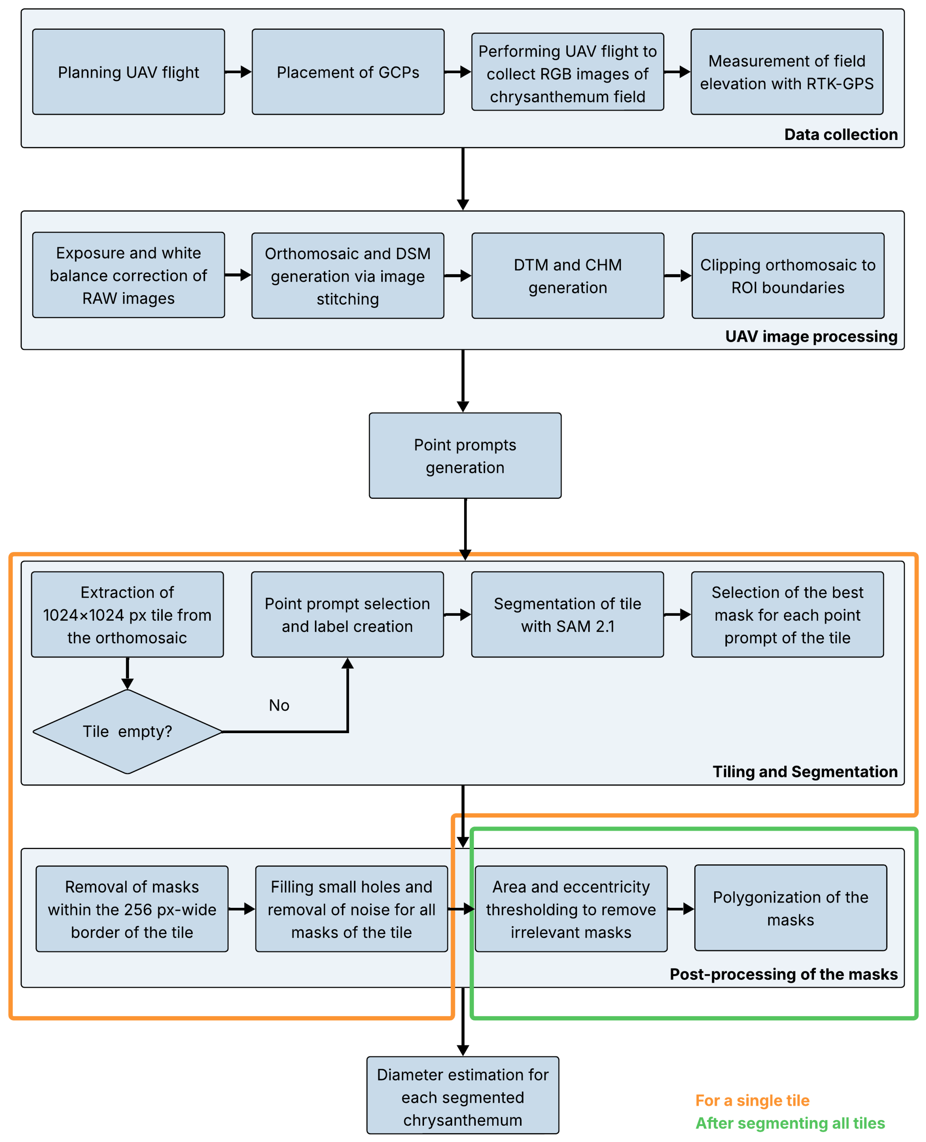
An overview of the pipeline is presented in Figure 1, with a more detailed version available in Appendix A (Figure A1). The process began with a UAV flight to capture high-resolution RGB images of the chrysanthemum field. Since the entire field could not be covered in a single high-resolution image, multiple overlapping images were taken and subsequently corrected and stitched to generate an orthomosaic of the field. In addition, a CHM, representing the height of the objects (plants and weeds) in the field, was calculated by subtracting the digital terrain model (DTM) from the digital surface model (DSM). Next, individual plants were segmented using SAM 2.1. For computational reasons, the orthomosaic was first divided into 1024x1024 pixel sections, referred to as tiles, before being inputted into the model. To avoid the segmentation of weeds and soil, the locations of the plants were determined based on local maxima in the CHM and these coordinates were used as prompts for the segmentation. Lastly, the model’s predicted masks were post-processed to improve the quality. These masks could then be used to extract various traits for each segmented plant. In this study, the crown diameter of a chrysanthemum was determined. A single plant pot contained multiple chrysanthemum cuttings. In this article, the terms plant and (ball-shaped) chrysanthemum refer to the collective group of cuttings grown together in a single pot, sold as a unit.

2.1. Study Area

The observed area was part of a 5.2 ha chrysanthemum field (Chrysanthemum morifolium (Ramat)) located in Staden, West Flanders, Belgium (50°57’2” N, 3°04’31” E). The field is organized into blocks spaced approximately 16 m apart, each comprising five beds of five rows. Around 4200 different genotypes, featuring a range of flower colors, including green, white, yellow, orange, red, pink, and purple, were grown under open-field cultivation. In week 19 of 2024, chrysanthemum cuttings were planted in trays and after a three-week rooting period, they were transplanted into plant pots. Two weeks later, in week 24, the plants were transferred to the field. No fertilization was applied; only irrigation was provided.
For the diameter measurements, two regions of interest (ROIs) were selected (Figure 2), each consisting of a single block of five beds containing chrysanthemums of various genotypes and flower colors. The growth stage of the plants varied, ranging from budding to flowering stages. ROI 1 covered an area of 3290 m 2 and ROI 2 an area of 2868 m 2 . The total number of plants within each ROI is provided in Table 1. Image acquisition of the field was performed twice: in week 41 on 8 October and one week later on 15 October. Data were collected on two separate dates to introduce greater variation into the dataset, reflecting conditions likely to be encountered in practical applications, such as variations in lighting conditions.

2.2. Data Collection

On 8 October and 15 October 2024, UAV flights were performed to collect high-resolution RGB images of the chrysanthemum field. On the first date, two flights were carried out, one at 11:03 a.m. and the other at 12:25 p.m., each covering a different ROI. On the second date, the entire study area was captured during a single flight, performed around 12:42 p.m. The cloud cover and hence lighting conditions varied between the flights. The second flight on 8 October and the flight on 15 October took place under broken cloud cover (7/8), while the first flight on 8 October was performed under scattered cloud cover (2/8), causing shadow across the field.
For all flights, the Matrice 600 Pro (DJI, Shenzhen, China) equipped with an RGB (visible spectral range) camera with 6000 × 4000 pixels and a 35 mm lens (Sony α 6400, Sony Corporation, Tokio, Japan) was used. The camera was mounted on the UAV using a gimbal to orient the camera in the nadir position during image collection. Images were taken with 80% overlap in both flight and lateral directions. The ground sampling distance (GSD) was 3.71 mm/px, 3.74 mm/px, and 3.84 mm/px for the first flight on October 8, the second flight on October 8, and the flight on October 15, respectively. The flight height and drone speed varied between the flights and are listed in Table A1. Shutter speed, aperture, and ISO were manually set before each flight and remained the same during the entire flight (Table A2). Each image was saved in both JPEG and RAW formats.
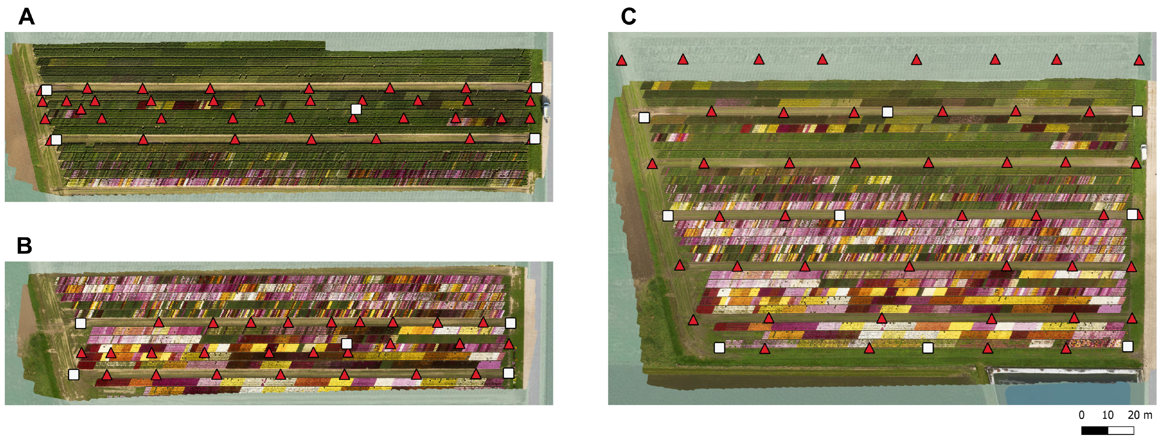
For georeferencing purposes, ground control points (GCPs) were laid out uniformly across the study area prior to each flight and their exact locations were determined using a real time kinematic (RTK) GPS (Stonex S10 GNSS, Stonex SRL, Milan, Italy). In addition, the latitude, longitude, and elevation of several other regularly spaced points were measured to generate a more precise DTM. The location of these points and the GCPs are visualized in the corresponding orthomosaics in Figure 3.

2.3. UAV Image Preprocessing

White balance and exposure of the RAW images of a single flight were corrected in Adobe Lightroom Classic (Adobe, San Jose, CA, USA) using a gray card (18% reference gray, Novoflex Präzisionstechnik GmbH, Memmingen, Germany) that was photographed during the flight. After correction, georeferencing and stitching were carried out in Agisoft Metashape Professional Edition (Agisoft 2.1.1 LCC, Saint Petersburg, Russia), resulting in an orthomosaic and DSM per flight, which were saved as GeoTIFF files. The orthomosaic was clipped using the package Rasterio v1.4.3 [38] to extract the data within the ROI. As the field was imaged on two separate dates and two distinct ROIs were selected, a total of four clipped orthomosaics were generated. On 15 October, both ROI 1 and ROI 2 were captured during a single flight, resulting in a single orthomosaic comprising both areas. However, on 8 October, two separate flights were performed to capture the two ROIs. As a result, ROI 1 was clipped from the orthomosaic of the 11:03 a.m. flight, while ROI 2 was clipped from the orthomosaic of the 12:25 p.m. flight.
A DTM was generated per flight using the elevation data from both the GCPs and additional measured field points. First, a regular grid with a resolution of 1 cm was constructed over the entire area of the input points. Elevation values at each grid node were estimated using linear barycentric interpolation within the triangles formed by applying Delaunay triangulation to the input points [39]. A DTM was also generated using only elevation data from the GCPs, and with reduced resolution, in order to evaluate the impact on segmentation performance and the accuracy of diameter estimation (Appendix B.1). The CHM was derived by subtracting the DTM from the DSM. Since the extent of the DSM was defined by the coverage of the UAV flight and the extent of the DTM was limited to the outermost points measured using the RTK GPS, the two surfaces did not fully overlap. To ensure accurate subtraction, both the DSM and DTM were reprojected to a common raster grid, defined by the intersection between them and the lowest resolution of the two datasets. Reprojection was performed with the package Rasterio v1.4.3 [38] using bilinear interpolation. The resolution of the DSM, DTM, and CHM per flight is listed in Table 2. The accuracy of the CHM produced using this method was validated in an earlier study by Borra-Serrano et al. [40].

2.4. Point Prompts Generation

Positive point prompts, corresponding to the location of the plant tops, were used to define the objects for segmentation. For each ROI and each flight date, a different set of point prompts was generated by identifying local maxima in the CHM, applying the image processing library Scikit-image v0.25.2 [41]. To avoid multiple prompts per plant and prompts corresponding to background, such as weeds or soil, the minimum allowed distance between local maxima and the minimum peak height were manually set until only points corresponding to the plants were obtained, based on a visual inspection. The minimum peak height was defined as a user-defined quantile of all positive height values within the ROI, which, for our experiment, was set to 0.3 quantiles. The value for the minimum distance between local maxima was 10 pixels for the four point prompts generations. The impact of these parameters on segmentation accuracy and diameter estimation performance is discussed in Appendix B.2.
The point prompts were originally defined as array indices within the CHM. To convert these indices to corresponding positions on the clipped orthomosaic, the array indices were first transformed into geographic coordinates using the affine transformation matrix of the CHM. Subsequently, these geographic coordinates were converted into array indices of the clipped orthomosaic by applying the inverse transformation using the affine transformation matrix of the clipped orthomosaic. Figure 4B presents an example of the generated point prompts for a small part of the orthomosaic of 15 October.

2.5. Tiling and Segmentation

Since the clipped orthomosaics were too large to be segmented in a single pass, they were divided into tiles of size 1024 x 1024 px (Figure 4A), which corresponded to the default input size of the SAM 2.1 encoder. The tiling was performed with 50% overlap in both vertical and horizontal directions to ensure accurate plant segmentation masks, including those at the borders of each tile. The plant rows did not align with the image borders because the orthomosaic was aligned with the true north, while the rows were not, resulting in tiles containing only nodata values. These were excluded from further processing to save memory and reduce computation time. For each remaining tile, point prompts located within the tile, including those on the tile border, were selected (Figure 4B). Positive labels (1) were generated for these prompts. Each individual tile, along with its corresponding prompts and labels, was given as input to the Image Predictor of the segmentation model SAM 2.1 [37]. The Hiera-L model was selected as an image encoder due its higher accuracy compared to smaller options. Segmentation performance and diameter estimation accuracy for the different SAM 2.1 encoders is presented in Appendix B.4. For each point prompt, three segmentation masks were generated, but only the mask with the highest quality score, as predicted by SAM 2.1, was selected (Figure 4C).

2.6. Post-Processing of the Masks

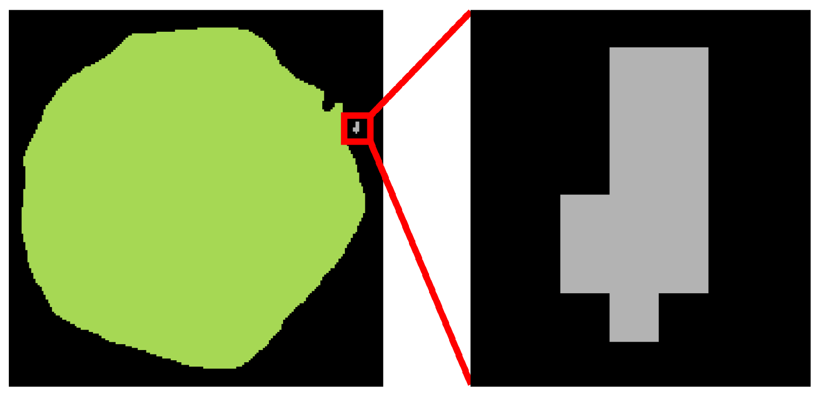
As a result of the tiling, plants at the borders of a tile were split over multiple tiles. Plant segmentation masks containing only pixels within the 256-pixel-wide border of the tile were excluded to prevent the presence of masks corresponding to fragmented plants in the field-level segmentation mask (Figure 4D). The quality of the remaining segmentation masks was improved by filling small holes using the binary fill holes function from the SciPy library (version 1.15.2) with default parameters [39]. Although the mask predicted by the segmentation model corresponded to a single object, it sometimes contained multiple connected regions, as illustrated in Figure 5. Since a ball-shaped chrysanthemum is a coherent structure, only the largest connected component of the mask, identified through connected component analysis using SciPy v1.15.2 [39], was maintained.
After segmenting all tiles of an orthomosaic, low-quality masks and those corresponding to non-target objects were filtered out based on thresholds for the eccentricity (upper threshold) and area (lower and upper threshold). These features were computed using the package scikit-image [41]. For both the eccentricity threshold and the area thresholds, various values were tested per orthomosaic until the desired result was achieved. Appendix B.3 provides a detailed assessment of how these parameters affected both segmentation performance and diameter estimation accuracy. Eccentricity was defined as the ratio of the focal distance to the major axis length, yielding a value between 0 and 1, with 0 indicating a perfect circle. Considering that ball-shaped chrysanthemums typically have a nearly circular shape, a mask with a high eccentricity value was unlikely to correspond to a chrysanthemum. The threshold value for eccentricity was 0.75 for all four clipped orthomosaics. Plant segmentation masks with areas that were either excessively large or small were also unlikely to represent a single plant and were therefore excluded. To identify these outliers, area thresholds were defined based on the interquartile range (IQR): the upper threshold was set as 3 times the IQR above the third quartile (Q3), while the lower threshold was set as 3 times the IQR below the first quartile (Q1).
As a result of the 50 % overlap between tiles, individual plants appeared in multiple tiles, resulting in multiple plant segmentation masks for the same plant. To retain a single mask per plant, an iterative procedure was applied. All masks were first sorted by descending area, and the iterative procedure started with the first mask of the sorted masks, corresponding with the largest mask. All masks with at least 80% of their area contained within this mask were considered to represent the same plant. Among these masks, the one with the highest quality score was selected as the final segmentation mask for that plant, and all these masks were excluded from future iterations to prevent duplicate detections. The quality score represented the predicted intersection over union (IoU) and was computed by SAM 2.1 during the segmentation process. This process was repeated for each subsequent mask, considering only those that had not previously been excluded. In each iteration, only the remaining, unprocessed masks were compared to the current one to check for overlap. The final selected plant segmentation masks were converted into polygons and saved as a GeoDataFrame. To transform the binary masks into polygons, the contours of the masks were first extracted using OpenCV v4.11.0 [42]. The masks were then converted into polygons and validated using the package Shapely v2.0.7 [43].

2.7. Diameter Measurement

The crown diameter of each segmented plant was calculated as the diameter of a circle with an area equal to that of its corresponding post-processed mask since the shape of a ball-shaped chrysanthemum closely resembles that of a circle. Additionally, this approach was selected for its reduced sensitivity to shape extremities (e.g., more elongated, oval-shaped chrysanthemums), as opposed to using the diameter of the smallest enclosing circle.

2.8. Analysis of the Data

Segmentation, post-processing, and diameter measurements of the chrysanthemum crowns were performed on each clipped orthomosaic. Since the field was imaged on two separate dates and two distinct ROIs were selected, a total of four analyses were conducted.

2.8.1. Evaluation of the Post-Processed Field-Level Segmentation Mask

To evaluate the quality of the segmentation and post-processing, the recall (Equation (1)), precision (Equation (2)), and F 1 score (Equation (3)) were calculated. False negatives were defined as plants without a mask, while false positives corresponded to masks that either did not overlap a chrysanthemum or had a visually estimated IoU below 0.8. A threshold value of 0.8 was selected as masks exceeding this threshold demonstrated a visually acceptable fit, and it was believed that the corresponding diameter measurements would fall within the range of variability expected in practical applications. Since no ground truth masks were available, the IoU was estimated through visual inspection rather than calculated. False positives and false negatives were manually counted by overlaying the post-processed field-level segmentation mask on the corresponding orthomosaic in QGIS (QGIS Desktop 3.40.0, Bratislava) [44]. Each chrysanthemum was evaluated by first verifying the presence of a segmentation mask and, if one was present, the IoU was visually estimated by assessing how much of the plant was not covered by the mask and/or the degree to which the mask extended beyond the boundaries of the plant. The IoU was therefore considered an approximate rather than an absolute value. However, as most plants either lacked a mask entirely or had a mask that closely matched the outline of the plant, evaluation using this method was considered feasible. The true positives, corresponding to masks with an IoU of at least 0.8, was computed as the difference between the total number of masks and the false positives.
recall = true positives true positives + false negatives
precision = true positives true positives + false positives
F 1 = 2 × precision × recall precision + recall

2.8.2. Evaluation of the Diameter Measurement

Field measurements of the chrysanthemum diameter were not provided. Therefore, no ground truth was available to compare the predicted diameters with. To evaluate the accuracy of the proposed pipeline, 102 chrysanthemums distributed across three selected sections (sections 1, 3, and 6 in Figure 7) in ROI 2 were manually measured in QGIS and compared with the computed diameters. The chrysanthemums inside a section were selected using a systematic sampling approach, in which every second plant was measured, to ensure a representative distribution. The manual diameters were defined as the mean of the largest crown diameter and the diameter perpendicular to it, measured directly on the orthomosaic with QGIS. To prevent bias, segmentation masks were not displayed during the measurement process.
The predicted crown diameters were compared for the same plants across both flight dates. Both ROI 1 and ROI 2 were captured twice, with a one-week interval between acquisitions. Polygons representing the same plant across the two imaging dates were matched based on the value for the IoU, defined as the ratio of the overlapping area to the total combined area of the two polygons. For each polygon, the IoU was calculated with all polygons from the other date, and the polygon with the highest IoU was selected as the match, but only if it exceeded 50%.

2.9. Sensitivity Analysis

A sensitivity analysis was performed to analyze the impact of manual settings on segmentation quality and diameter estimation. This included the evaluation of parameters used for point prompt generation—minimum peak height and minimum distance between local maxima (Section 2.4)—and for mask post-processing—upper eccentricity threshold and upper and lower area thresholds (Section 2.6). In addition, the influence of the DTM resolution and the number of elevation points used in its calculation was evaluated. Since the resolution of the CHM was determined by the lowest resolution between the DSM and DTM, changes in DTM resolution directly affected the CHM. Finally, different encoders of SAM 2.1 were tested.
To automate the evaluation, a ground truth mask was created for all plants that contained at least a part within the sections visualized in Figure 7. The annotation was conducted in QGIS by manually drawing polygons on top of the orthomosaic of 15 October in freehand mode, and a total of 480 plants were evaluated. Predicted masks were compared against this ground truth to compute true positives (IoU ≥ 0.8), false negatives (no match with IoU ≥ 50%), and false positives (remaining predicted masks). Recall, precision, and F 1 score were calculated as defined in Equations (1)–(3). The diameter estimations were evaluated by comparing predicted values to manual measurements (Section 2.8.2). Due to the labor-intensive annotation process, the sensitivity analysis was only performed for data collected on 15 October within ROI 2. This field was chosen for its diversity in plant size, flower color, and the presence of weeds and grass.

2.10. Computational Resources

The experiments were performed on a system running Windows Server 2022 Standard Edition, equipped with 384 GB RAM, two Intel Xeon Gold 6226R CPUs and an NVIDIA RTX A5000 GPU. Wall time and peak RAM usage were measured for processing ROI 1 of the orthomosaic acquired on October 15, covering the entire processing pipeline. The DTM was generated using elevation data from 55 points and covered an area of 2.00 ha, while the resulting CHM spanned 1.84 ha. The clipped orthomosaic was divided into 3913 tiles, of which 879 were segmented with SAM 2.1 using the Hiera-L encoder. The remaining tiles contained only nodata values due to the orientation of the clipped orthomosaic aligned to true north and were not processed. For each of the 8589 point prompts, three masks were predicted. The total processing time was 25 min, with tiling and segmentation accounting for the majority of the time (88%). The remaining time was distributed across the following steps: DTM generation (2%), CHM calculation (5%), point prompt generation (1%), post-processing (3%), and diameter estimation (1%). Peak RAM usage reached 23 GB during segmentation.

3. Results

3.1. Evaluation of the Post-Processed Field-Level Segmentation Mask

To estimate the crown diameter of each chrysanthemum, segmentation masks were generated for each ROI and flight date. Across the four clipped orthomosaics, 96.86% of the plants were successfully segmented. Background segmentation was negligible, with only one instance observed across all four field-level segmentation masks. In eleven cases, the predicted masks covered only half of a chrysanthemum, leading to a visually estimated IoU below 0.8. These twelve false positives resulted in a precision of 99.96% across the two ROIs and both flight dates. A detailed summary of the segmentation performance for each ROI per flight date is presented in Table 3.
According to the recall results, a lower proportion of chrysanthemums were segmented in ROI 2 compared to ROI 1. Since ROI 2 contained more chrysanthemums at the flowering stage and a larger number of non-green flowers, it is possible that the segmentation model experienced more difficulties in accurately segmenting colorful, blooming plants. Alternatively, the flowering chrysanthemums had an increased canopy size, leading to greater overlap between neighboring plants and reduced inter-plant spacing, thereby complicating individual crown segmentation. However, visual inspection revealed that the majority of chrysanthemums that were not segmented were in the bud stage, resembling those shown in Figure 6. Furthermore, precision remained consistent across the two flight dates within the same ROI, despite increased blooming observed on October 15 compared to October 8. This suggests that flowering did not negatively impact the pipeline’s performance.
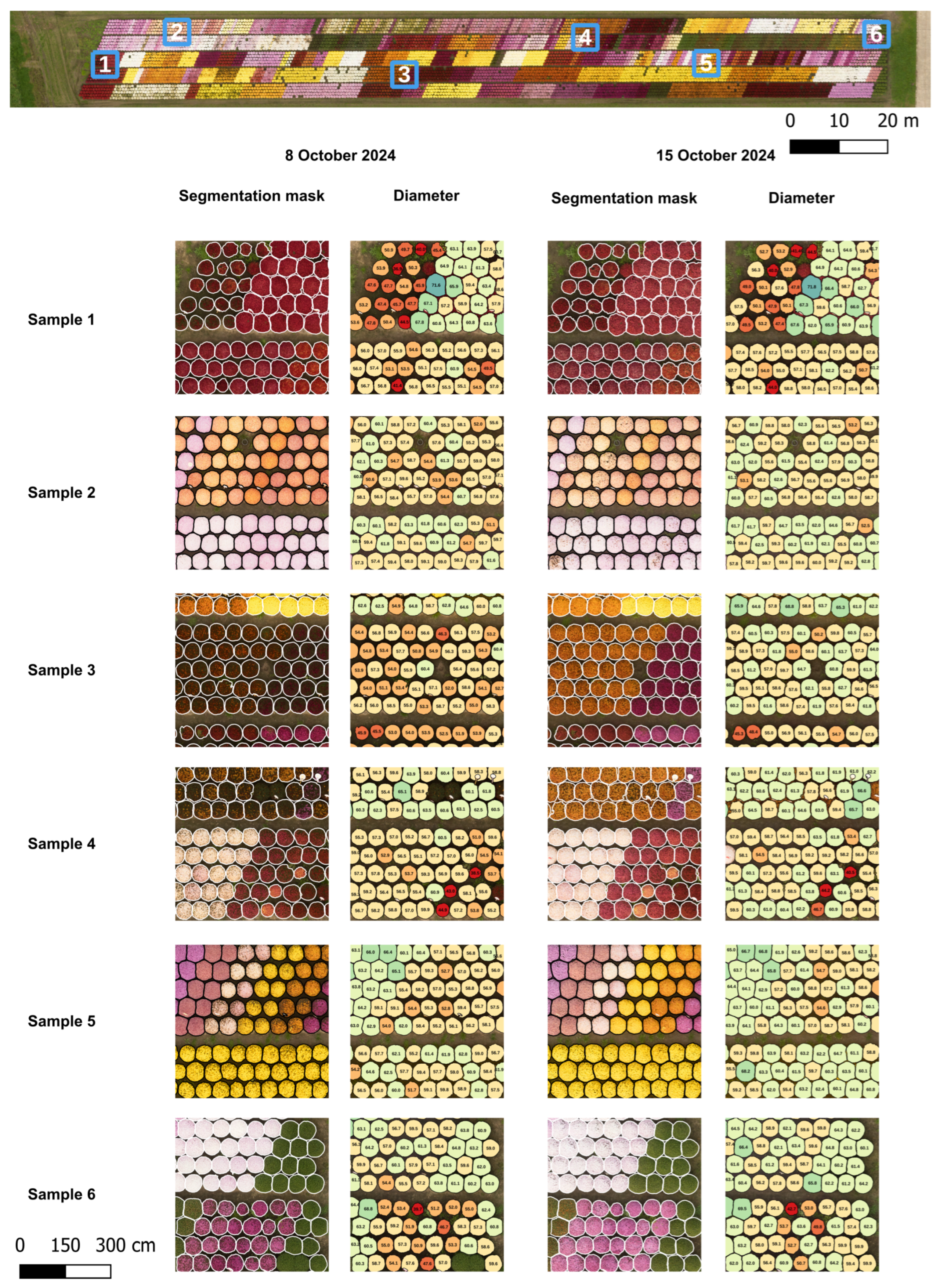
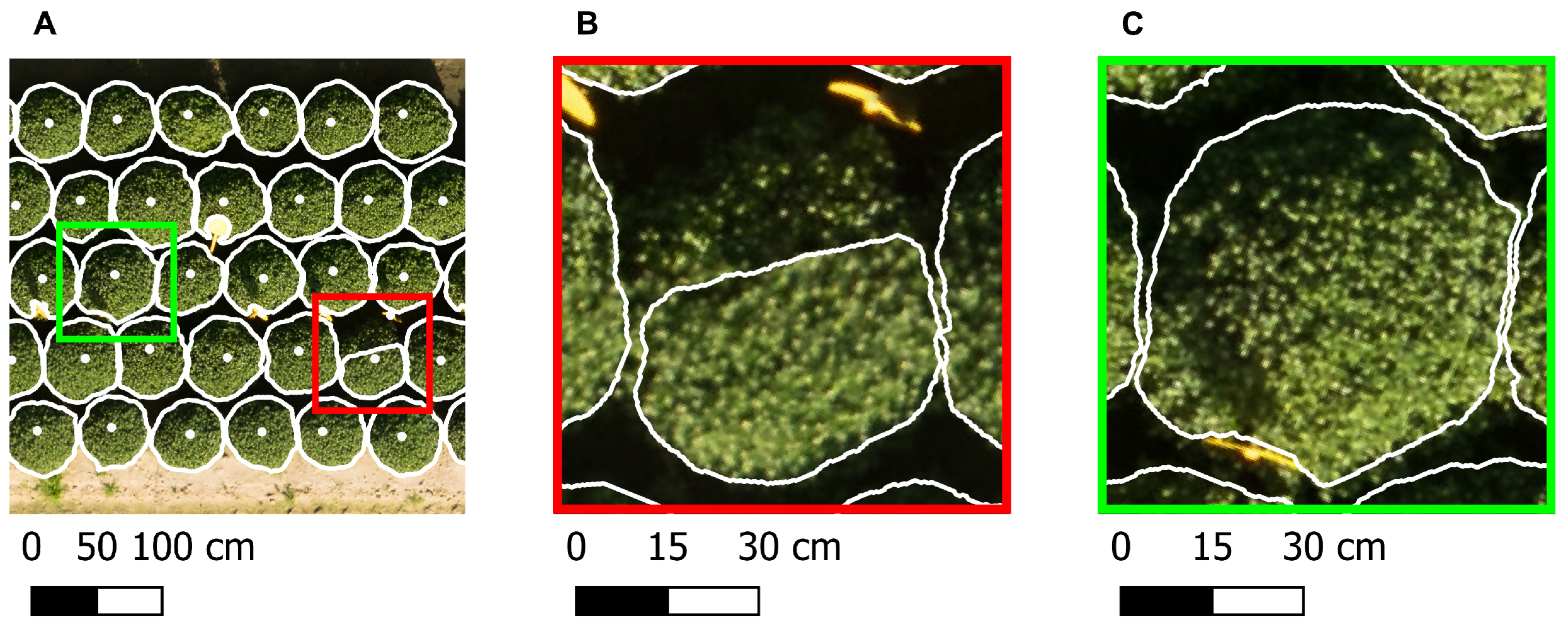
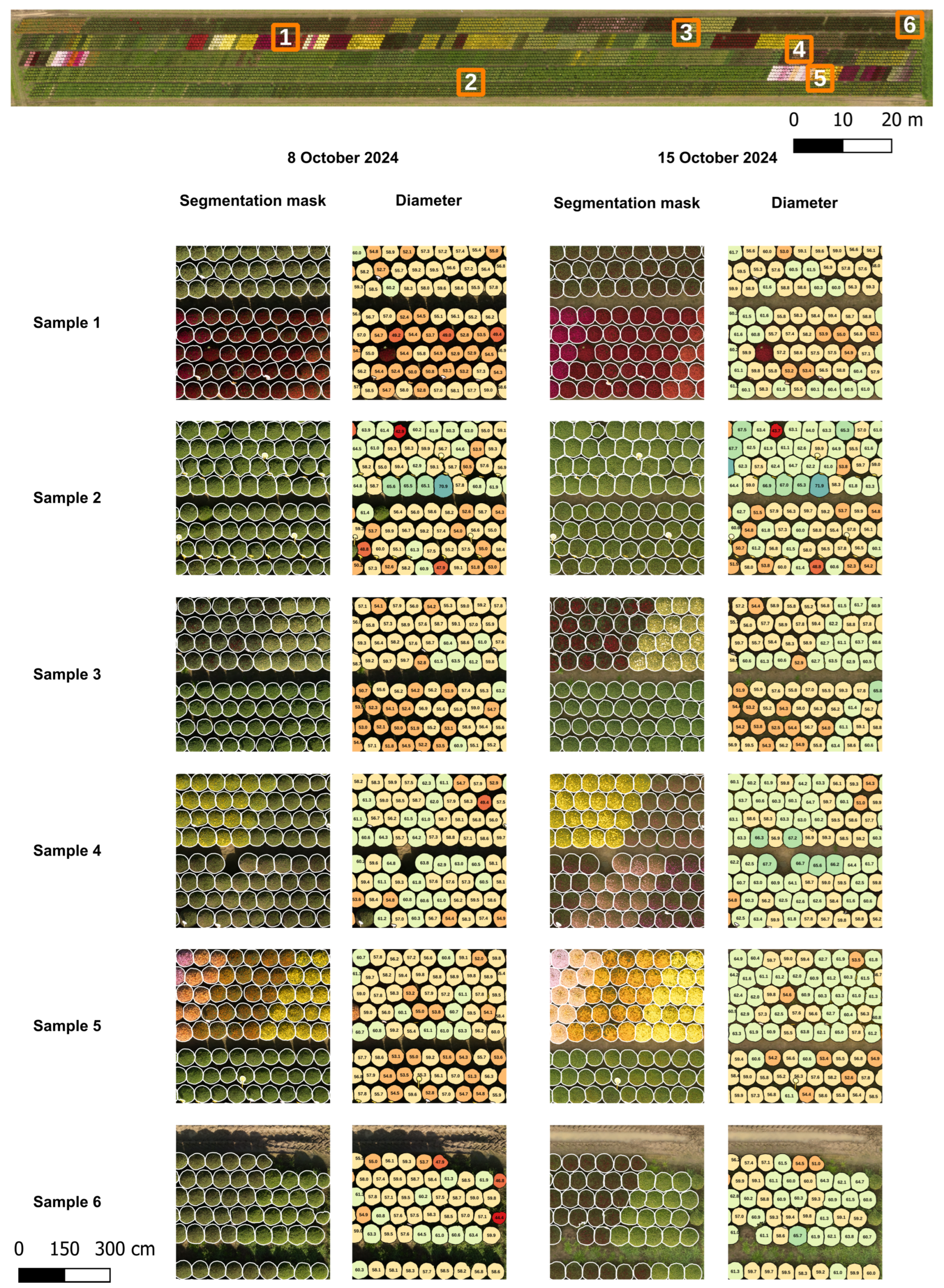
A visual inspection of the post-processed field-level segmentation masks was performed to gain a more detailed understanding of the false positives and false negatives. Zoomed-in examples from selected sections of ROI 2 are shown in the “Segmentation mask” column of Figure 7. For ROI 1, the masks of selected sections are shown in Figure A3. In general, the segmentation masks closely followed the outlines of the chrysanthemums, even in cases where the plants were in contact with each other. However, when chrysanthemums formed a continuous, overlapping canopy, accurate segmentation was not always achieved. In some instances, particularly within ROI 1 of the orthomosaic acquired on October 8, the masks covered only approximately half of the plant. The flight over ROI 1 on October 8 was conducted under scattered cloud cover, resulting in field shadows and thus color variation (Figure 8). Closer inspection revealed that these partial masks corresponded to plants that were partially shaded, with the segmentation predominantly applied to the non-shaded portions, as shown in Figure 8B. Nevertheless, the model was able to handle orthomosaics captured under variable cloud cover conditions, as the majority of shaded plants were correctly segmented, of which an example can be found in Figure 8C.
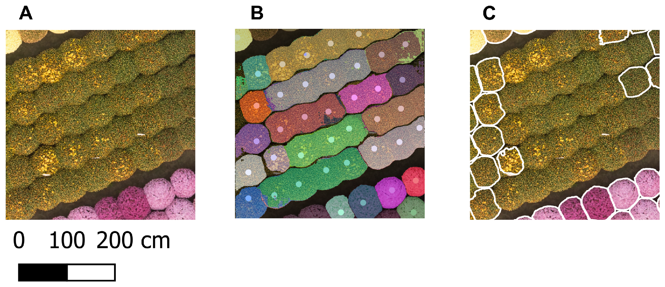
As illustrated in the figures (Figure 7 and Figure A3), the algorithm showed robustness to variations in flower color and morphology, effectively handling differences in size and shape, including both more rounded and more elongated crowns. Unsegmented chrysanthemums were often found in clusters, suggesting that the model may have had difficulties segmenting certain genotypes or growth stages. Larger, non-segmented clusters typically consisted of partially flowering chrysanthemums that formed an almost continuous overlapping canopy, as shown in Figure 6. In most cases, the absence of a mask for a chrysanthemum was due to incorrect prediction by the segmentation model, as demonstrated by Figure 9. The mask predicted by the segmentation model for one point prompt (= one chrysanthemum) covered multiple chrysanthemums, probably because the plants were very close to each other. Since the area of the mask was substantially larger than the average plant mask area, it was removed during post-processing and, therefore, the chrysanthemum did not have a mask in the field-level segmentation mask.
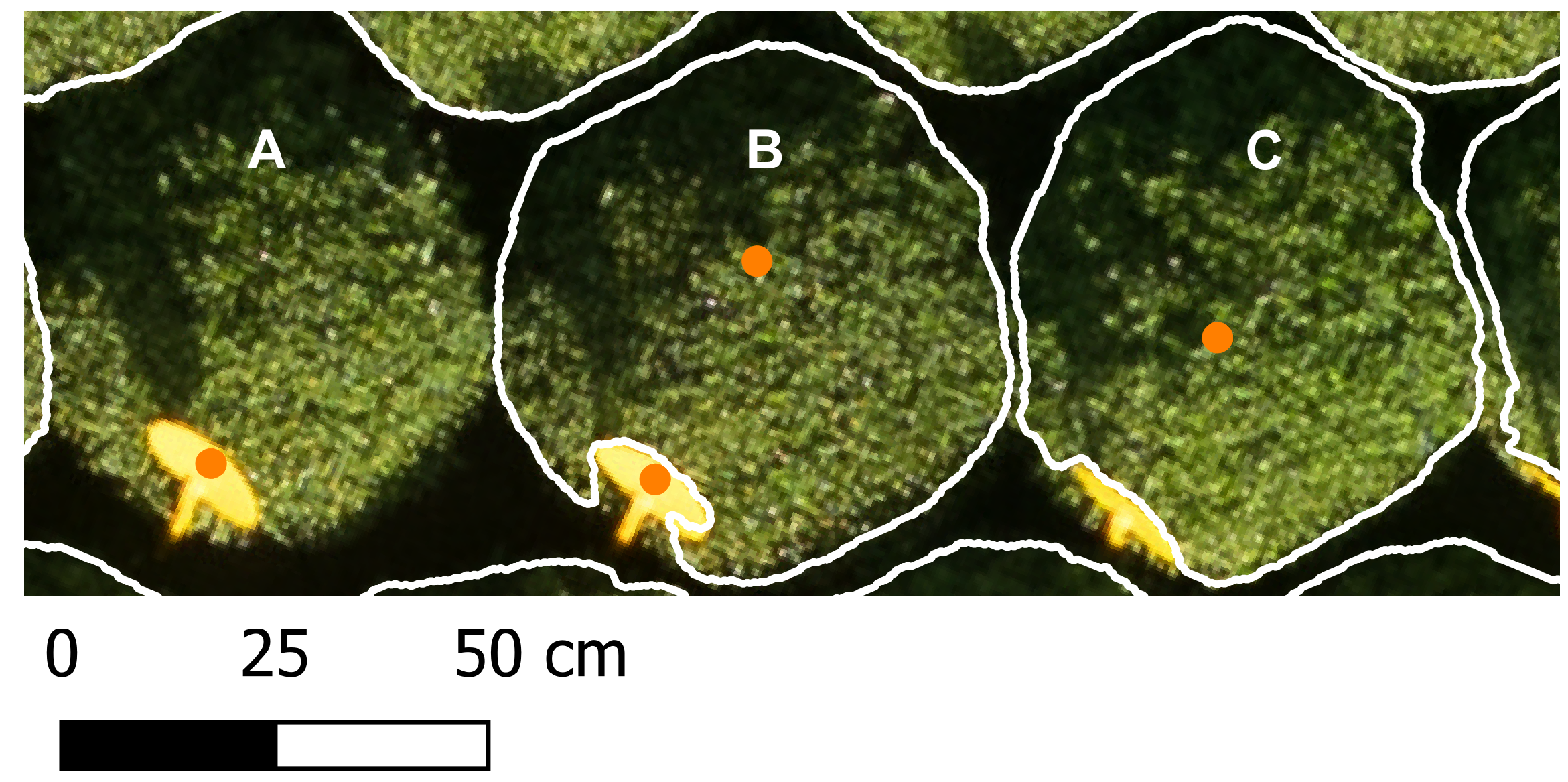
However, in some instances, no mask was predicted because no point prompt was provided. The absence of a point prompt for a chrysanthemum was likely due to the chosen parameter values for the local maxima calculation. In contrast, sometimes a point prompt was generated but it was not located directly on the plant itself. A possible cause is the plastic plant labels inserted into certain pots. These labels extended slightly above the top of the plants and could therefore correspond to local maxima, resulting in the generation of a point prompt. Typically, separate prompts were generated for both the plant and the label, with the label’s segmentation mask being removed during post-processing due to its smaller size (Figure 10B). However, in cases where a chrysanthemum was particularly small and the label was positioned near the center of the plant, only the label would receive a point prompt (Figure 10A). This occurred because a minimum distance between local maxima was required, potentially causing the plant’s own local maximum to be overlooked. On the other hand, the only instance where a mask corresponded to background was caused by a point prompt positioned at the border of a plant label. This led the model to predict a mask for the background rather than for the plant label. Since the area of the mask fell within the area threshold range, it was not removed during post-processing. The influence of plant labels on point prompt generation and segmentation performance was evaluated within the sections shown in Figure A3 and Figure 7 for both acquisition dates. Of the 162 plant labels, 86 (53%) had a point prompt located on them. These 86 prompts represented approximately 5% of the total point prompts generated. However, none of the plant labels had a mask after post-processing.
Figure 7. Segmentation masks and diameters for various sections (blue squares) of ROI 2, captured on 8 October and 15 October. The selected sections represent a range of chrysanthemum color and size variations. The values within the plant segmentation masks correspond with the estimated chrysanthemum diameters (cm), ranging from small (red mask) to large (blue mask).
Horticulturae 11 01043 g007
Figure 8. Segmentation performance for shaded areas of the field. (A) Section of the orthomosaic from ROI 1, captured on 8 October. The UAV flight was performed under scattered cloud cover, resulting in shadow across the field. The white dots represent the point prompts used to guide SAM 2.1. (B) Plant segmentation mask covering only part of the plant due to the presence of shadow. (C) Partially shaded chrysanthemum that was correctly segmented.
Horticulturae 11 01043 g008
Figure 9. Illustration of an inaccurate prediction caused by the segmentation model itself, rather than prompt generation or post-processing steps. (A) Tile of the orthomosaic captured on 15 October. (B) Segmentation mask for the tile, generated by SAM 2.1, prior to any post-processing. The point prompts are shown as white dots, indicating that a prompt was generated for each individual plant. However, several masks overlapped multiple plants. Distinct colors represent different masks. (C) Final segmentation mask for the tile after post-processing. Plant masks covering multiple plants were removed based on area and eccentricity thresholds.
Horticulturae 11 01043 g009
Figure 10. Illustration of possible scenarios for point prompt generation in case a plant label was inserted in the plant pot. Orange dots indicate the point prompts, while white outlines represent the individual plant masks. (A) A point prompt was generated only for the label as it was positioned near the center of the plant and extended above it. (B) Point prompts were generated for both the label and the plant. (C) A point prompt was generated only for the plant as the label was lower in height and did not form a distinct peak.
Horticulturae 11 01043 g010

3.2. Evaluation of the Diameter Measurement

In the absence of ground truth values obtained through field measurements, the accuracy of the pipeline for automated chrysanthemum crown diameter measurement was evaluated by comparison with manual measurements performed in QGIS. The results of this comparison are presented in Figure 11, covering both flight dates. In both scatter plots, the majority of data points are located close to the 1:1 reference line, distributed both above and below it, indicating that the predicted diameters were sometimes bigger and sometimes smaller than the measured values. The MAE and RMSE were 1.57 and 2.22 for 8 October, and 1.90 and 2.49 for 15 October, respectively. These results suggest that the pipeline provided an accurate estimation of the chrysanthemum crown diameter, which is further supported by the coefficient of determination ( R 2 ). The value for R 2 was approximately 0.90 for both dates, indicating a relatively high level of agreement between the automated and manual approach.
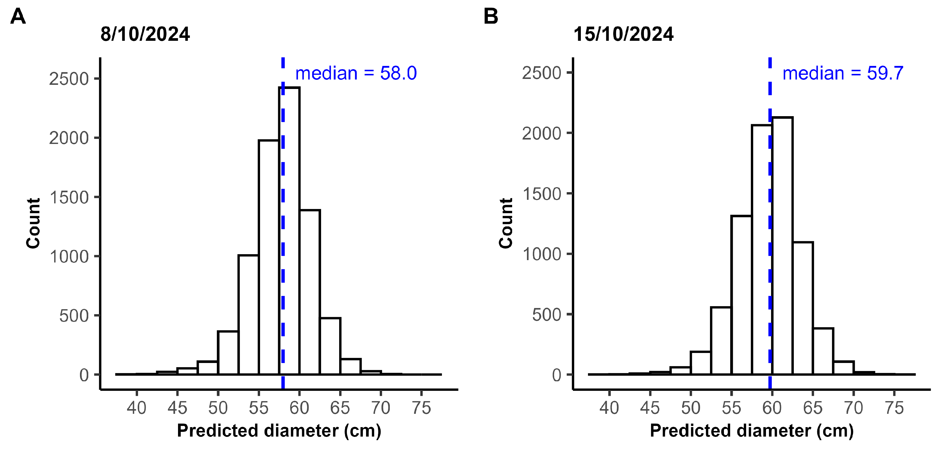
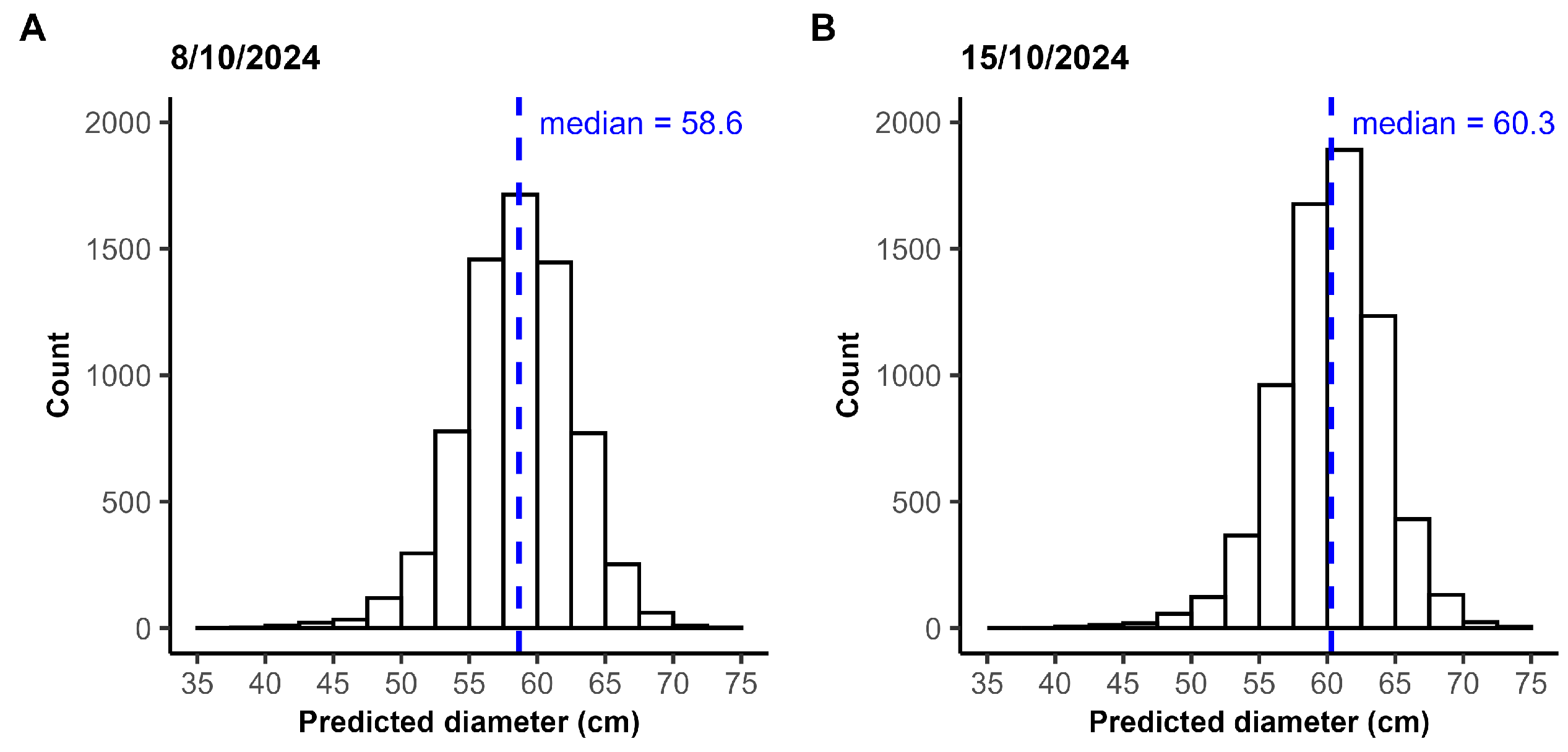
The same chrysanthemums were evaluated on two dates, one week apart. The distribution of the predicted diameter within ROI 2 is given in Figure 12 for both flight dates. The corresponding histograms for ROI 1 are presented in Figure A2. For chrysanthemums in ROI 1, the predicted diameters ranged from 39.0 cm to 71.3 cm on 8 October, with a median of 58.0 cm, and from 38.1 cm to 75.1 cm on 15 October, with the median increasing to 59.7 cm. For chrysanthemums in ROI 2, the diameters ranged from 36.1 cm to 73.3 cm on 8 October and from 40.0 cm to 74.5 cm on 15 October, with the median increasing from 58.6 cm to 60.3 cm. The results showed a slight increase in chrysanthemum diameters over the one-week period, as indicated by rising median values and a visible rightward shift in the histograms. To determine whether the observed changes were statistically significant and not attributable to model noise or natural variability, a one-tailed paired t-test was performed with a significance level of α = 0.05. For ROI 1, a statistically significant increase in diameter was observed at time point 2 (M = 59.55, SD = 3.73) compared to time point 1 (M = 57.79, SD = 3.56; t(7856) = 136.60, p < 0.001). Similarly, for ROI 2, there was also a statistically significant increase in diameter at time point 2 (M = 60.12, SD = 3.88) compared to time point 1 (M = 58.44, SD = 4.10; t(6842) = 101.23, p < 0.001). Although much substantial growth was not expected within such a short time frame, the observed changes may be attributed to plant sagging associated with flowering. The difference between the two time points demonstrate that the proposed pipeline is sensitive enough to detect subtle variations in plant size.

3.3. Sensitivity Analysis

The results of the sensitivity analysis can be found in Appendix B.

4. Discussion

This study demonstrates the applicability of SAM 2.1, combined with point prompts derived from the CHM, for the automatic extraction of ornamental plant traits from UAV-acquired RGB images to support ornamental growers and breeders in their decision-making. A novel aspect compared to similar work is the label-free nature of the proposed pipeline. The approach requires no annotated data and no model training, making it significantly faster and less labor-intensive than traditional supervised segmentation methods. Certain conditions must be met for the pipeline to be applicable: a CHM must be available and the plants should be relatively compact and not form a continuous, overlapping canopy.
The availability of an accurate CHM is necessary to generate point prompts for identifying the objects of interest. In the absence of a CHM, the model cannot target specific objects and instead attempts to segment all visible elements in the image, leading to noise and irrelevant segmentations. On the other hand, when an inaccurate CHM is used, point prompts may be misplaced, resulting in masks that correspond to background rather than the intended plants. The accuracy of the CHM itself depends on the quality of the DSM as well as the DTM. A precise DSM requires UAV flights to be performed with sufficient image overlap [40,45]. While increasing image overlap enhances DSM precision, it also prolongs the flight duration, reducing the area that can be captured in a single flight without requiring a battery change. Nevertheless, the area that can be evaluated with this method is still considerably larger than what could be assessed with the traditional approach. Generating an accurate DTM requires measuring the elevation of evenly distributed points across the ROI, which requires an RTK-GPS, increasing overall costs, and increasing data collection time. However, as reported in Appendix B.1, no additional elevation measurements beyond the GCPs are required to obtain good results, provided the measured points cover the borders of the ROI and the terrain does not have abrupt slope changes. In addition, this measurement only needs to be performed once.
The method for generating point prompts relies on the detection of local height maxima. Consequently, non-target objects within the field that are equal to or taller than the target plants may also trigger prompt generation and subsequent segmentation. However, masks that deviate in size or shape are filtered out in the post-processing step, meaning that only non-target objects with characteristics similar to the target plants are likely to be retained. A potential solution to eliminate the need for point prompts and, thus, the CHM is to use PerSAM-F, a customized version of SAM that enables personalized object segmentation through one-shot fine-tuning [46]. Although the fine-tuning is completed within 10 s, it still requires one annotated image. To avoid manual annotation, Osco et al. [47] combined Grounding DINO with SAM to enable segmentation based on text prompts and compared this approach with the performance of SAM using point and bounding box prompts. The results indicated that text prompts generally resulted in lower segmentation accuracy, with point prompts proving more effective for identifying and segmenting small, individual objects. The performance of segmentation guided with text prompts relies on Grounding DINO’s ability to correctly interpret and localize textual descriptions within the image. The authors noted that this ability can be limited, especially when domain-specific terminology is not well represented in the model’s training data. In contrast, point prompts offer more direct control over the segmentation target, thereby improving reliability. In addition, the combination of Grounding DINO with SAM was applied to automatically generate a mask of the target object, which was then used to fine-tune PerSAM-F. The authors stated that the effectiveness of the approach depends on the accurate identification of the target object, as PerSAM-F cannot be fine-tuned in the absence of an initial segmentation. It remains uncertain whether this method is effective for the segmentation of ornamental plants. This can be further explored in future research. The CHM can also serve a purpose beyond generating point prompts. For instance, Rayamajhi et al. [12] used it to estimate the height of individual plants.
The captured field included chrysanthemums of various genotypes, flower colors, sizes, and growth stages. An average recall of 96.86% demonstrates that the model is robust to all these variations, making it suitable for automatic diameter measurement across different chrysanthemum genotypes, flower colors, and both the bud and flowering stage. Furthermore, shadow between as well as on the chrysanthemums did not pose major issues, as evidenced by the similar recall and precision between the flights over ROI 1 captured on 8 October and on 15 October. The two flights were carried out under different lighting conditions. The coefficient of determination ( R 2 ) and the MAE indicated a slightly imperfect match between the estimated and measured diameters, with the pipeline both underestimating and overestimating the crown diameter. It should be noted that the manual measurements used for comparison do not represent absolute ground truth and likely contain some degree of measurement error themselves related to the expert. Even if manual measurements were performed directly in the field rather than on the orthomosaic, some variability would remain, as different experts are unlikely to obtain identical diameter estimates for each plant.
Zhang et al. [26] estimated chrysanthemum crown diameter using the bounding rectangle of the segmentation mask predicted by Mask R-CNN. Their reported RMSE of 2.29 cm, based on comparisons between estimated diameters and manually measured field values obtained using a measuring tape, was comparable to the values obtained using our approach. However, Mask R-CNN is a supervised learning model and its application to varying field conditions typically requires retraining [34]. The researchers used a dataset containing 3014 annotated images with 3262 instances. Manually annotating that amount of data requires a substantial amount of time and labor. In contrast, our proposed method operates without the need for manual annotation or model training.
There are still some opportunities to further optimize the pipeline. For example, to avoid reliance on manual height measurements with the RTK GPS for DTM generation, an alternative approach could be to perform a flight before the chrysanthemums are present in the field, capturing the DTM of the terrain beforehand. In this case, an appropriate choice of sensor and flight parameters (flight altitude and overlap) is essential, as the resolution of the DSM and, consequently, the quality of the CHM depend on them. However, this would further reduce the manual labor. To be more user-friendly, the manual settings for the point prompt generation and post-processing could be specified using meaningful real-word metrics. For instance, instead of expressing the minimum distance between local maxima in pixels, defining this value in meters would be more intuitive, given that a reasonable estimation is often available. However, our findings indicate that these parameters primarily influence the segmentation performance (number of plants with/without a mask), rather than the accuracy of diameter measurements. Moreover, as long as the thresholds are not too strict, the segmentation performance remains satisfactory. Consequently, if sporadic errors are acceptable, the precise tuning of these manual settings becomes less critical. In this case, it is recommended to use low values for the minimum distance and peak height during point prompt generation and high values for maximum area and eccentricity, along with a low value for minimum area during post-processing.
For the segmentation, the largest model, Hiera-L, was selected as the SAM 2.1 image encoder due to its better segmentation accuracy, as reported in Appendix B.4. This performance advantage comes at the cost of a longer processing time; however, the additional time remains relatively limited (Table A3). In scenarios where fast processing is required, smaller image encoders (Hiera-S and Hiera-T) may serve as an alternative, but this comes with reduced segmentation performance and lower diameter accuracy.
Although the method has certain limitations, we believe it holds potential as a robust tool for the automatic extraction of various plant traits across different field conditions, with potential applications in both breeding (e.g., selection) and production (e.g., growth monitoring and stress detection) contexts. In future research, the algorithm could be applied to other crops, both in container fields and fields, to further test its robustness. Moreover, the predicted diameters could be validated against manual measurements performed by experts. In addition to diameter, other traits such as canopy volume and height could also be extracted. Monitoring these traits over time would allow for evaluation of the algorithm’s potential for supporting growth monitoring in a production environment, as illustrated by Vigneault et al. [48]. Moreover, when multispectral imagery is available, vegetation indices can be calculated on a per-plant basis to support yield and biomass assessments and the detection of biotic and abiotic stresses, including drought and diseases [19].

5. Conclusions

This study presented an approach for the robust, label-free segmentation of plants in UAV-acquired RGB imagery, enabling the automatic extraction of individual plant traits. Unlike supervised segmentation models commonly used in this context, the proposed approach eliminates the need for an annotated training dataset, significantly reducing the time and labor required to adapt the approach to new field conditions. This method enables objective, field-scale evaluation of plants without relying on traditional manual measurements. The extracted feature(s) can support plant growth monitoring and stress detection, providing valuable input for site-specific applications of water and pesticides. Additionally, the approach has the potential to assist breeders in their decision-making. Future research could explore the broader applicability of this method using UAV-derived imagery across different ornamental and horticultural crops, as well as its effectiveness in extracting a wider range of plant traits.

Author Contributions

Conceptualization, R.H., J.M., J.V.H., J.V. and P.L.; methodology, R.H., J.M., J.V.H., J.V. and P.L.; validation, R.H., J.M., J.V. and P.L.; formal analysis, R.H., J.M., J.V. and P.L.; investigation, R.H., J.M., J.V. and P.L.; writing—original draft preparation, R.H., J.M., J.V. and P.L.; writing—review and editing, R.H., J.M., J.V.H., J.V. and P.L.; visualization, R.H.; supervision, J.M., J.V. and P.L.; project administration, R.H., J.V.H. and P.L.; funding acquisition, J.V.H., J.V. and P.L. All authors have read and agreed to the published version of the manuscript.

Funding

This research was funded by VLAIO grant number HBC.2023.0922—SierTech—New technologies and artificial intelligence for optimal crop management in floriculture, a collaborative project between Viaverda, UGENT, and ILVO.

Data Availability Statement

The datasets presented in this article are not readily available because the data are part of an ongoing study. Requests to access the datasets should be directed to the corresponding author.

Acknowledgments

The authors wish to express their gratitude to Gediflora for their cooperation and for granting permission to perform UAV flights over their fields. They also wish to thank Isabel Roldán-Ruiz for the valuable insights that helped shape the direction of this work. Furthermore, they would like to thank Thomas Vanderstocken and Aaron Van Gehuchten for performing the UAV flights and Thomas Vanderstocken for stitching the UAV imagery.

Conflicts of Interest

The authors declare no conflicts of interest. The funders had no role in the design of the study; in the collection, analyses, or interpretation of data; in the writing of the manuscript; or in the decision to publish the results.

Appendix A. Supplementary Figures and Tables

Figure A1. Flow chart of the pipeline for automatic extraction of plant traits from UAV RGB imagery using label-free segmentation, demonstrated for crown diameter measurement of chrysanthemums.
Horticulturae 11 01043 g0a1
Table A1. Flight details for each UAV flight.
DateTimeCloud Cover (/8)Flight Height (m)Flight Speed ( m · s 1 )Overlap Flight Direction (%)Overlap Lateral Direction (%)Area ( m 2 )
8 October 202411:03 a.m.2/8 *36.73.1808011,500
8 October 202412:25 p.m.7/8 *33.13.080809140
15 October 202412:42 p.m.7/8 *36.53.1808023,700
* Cloud cover is quantified on an eight-point scale, where higher values indicate greater cloud coverage. A value of 2 corresponds to scattered cloud cover, meaning few clouds were present. In contrast, a value of 7 indicates broken cloud cover, where clouds obscured most of the sky, though it was not completely overcast. The area corresponds with the area surveyed by the UAV.
Table A2. Camera settings and number of images taken during each flight.
DateTimeShutter Speed ( s 1 )ApertureISONumber of Images
8 October 202411:03 a.m.1/1250f/3.2250481
8 October 202412:25 p.m.1/1250f/3.5320359
15 October 202412:42 p.m.1/1250f/3.52001394
Table A3. Comparison of wall time and peak RAM usage across the available SAM 2.1 encoders for segmentation of the clipped orthomosaic (ROI 1) acquired on October 15. The experiments were conducted on a system running Windows Server 2022 Standard Edition, equipped with 384 GB RAM, two Intel Xeon Gold 6226R CPUs, and an NVIDIA RTX A5000 GPU.
SAM 2.1 EncoderWall Time (s)Peak RAM Usage (GB)
Hiera-L encoder133323
Hiera-B+ encoder125224
Hiera-S encoder115923
Hiera-T encoder117019
Figure A2. Distribution of the predicted crown diameters (cm) for the chrysanthemums in ROI 1 on 8 October (A) and 15 October 2024 (B).
Horticulturae 11 01043 g0a2
Figure A3. Segmentation masks and diameters for various sections (orange squares) of ROI 1 captured on 8 October and 15 October. The selected sections represent a range of chrysanthemum color and size variations. The values within the plant segmentation masks correspond with the estimated chrysanthemum diameters (cm), ranging from small (red mask) to large (blue mask). The figure further demonstrates the applicability of the pipeline to orthomosaics acquired under suboptimal lighting conditions. Although shadows were present on and around the chrysanthemums, the segmentation masks remained accurate.
Horticulturae 11 01043 g0a3

Appendix B. Sensitivity Analysis

Appendix B.1. Effect of Simplified DTM on Segmentation Accuracy and Diameter Measurement

The influence of the number of elevation points used in the generation of the DTM on segmentation quality and diameter estimation was evaluated. In addition, various DTM resolutions were tested. The results are summarized in Table A4.
Generating a DTM using only GCPs reduced the elevation range, with the maximum height lowered and the minimum height raised. Despite this, the tops of the plants remained clearly visible in the CHM. Point prompts were largely consistent with the reference, except in one region lacking CHM data due to insufficient GCP coverage, resulting in missing segmentation masks and, thus, lower recall. Overall, slightly fewer plants received masks, but their shapes matched the reference exactly, so diameter estimation was unaffected.
Reducing the DTM resolution led to fewer point prompts, with some disappearing from both background elements (such as labels, weeds) and actual plants. Lower resolutions also shifted prompt locations, often toward the edge of the plant. The accuracy of point prompt placement proved critical: slight displacements led to missing masks in some cases, while, in others, new masks appeared where none existed in the reference.

Appendix B.2. Sensitivity Analysis of Parameters for Point Prompt Generation

The impact of the point prompt generation parameters, minimum peak height and minimum distance between local maxima, on segmentation performance and diameter estimation accuracy was analyzed. An overview of the results is presented in Table A5.
Reducing the minimum distance between local maxima increased the number of point prompts by approximately 4% at 5 px and 36% at 1 px compared to the reference. Occasionally, a plant that previously only had a point prompt located on the plant label also obtained one directly on the plant. Multiple point prompts per plant resulted in better segmentation, with more plants receiving a mask, indicated by the higher recall. In contrast, increasing the minimum distance between local maxima decreased the number of point prompts, with a decrease of 4% at 15 px compared to the reference. Although it primarily removed point prompts from plant labels, there was a slight reduction in the number of plants that were segmented. Further decreasing the distance led to a 17% decrease and a notable decline in recall due to missing masks.
Lowering the minimum peak height had a limited effect on point prompts located on plants but increased the number of prompts on the background, leading to more false positives. These occurred outside the evaluated regions, which explains the similar recall and precision values. Increasing the peak height threshold to the 0.9 quantile reduced the amount of point prompts to 44% of the reference, reducing the number of plants with masks and lowering the recall.
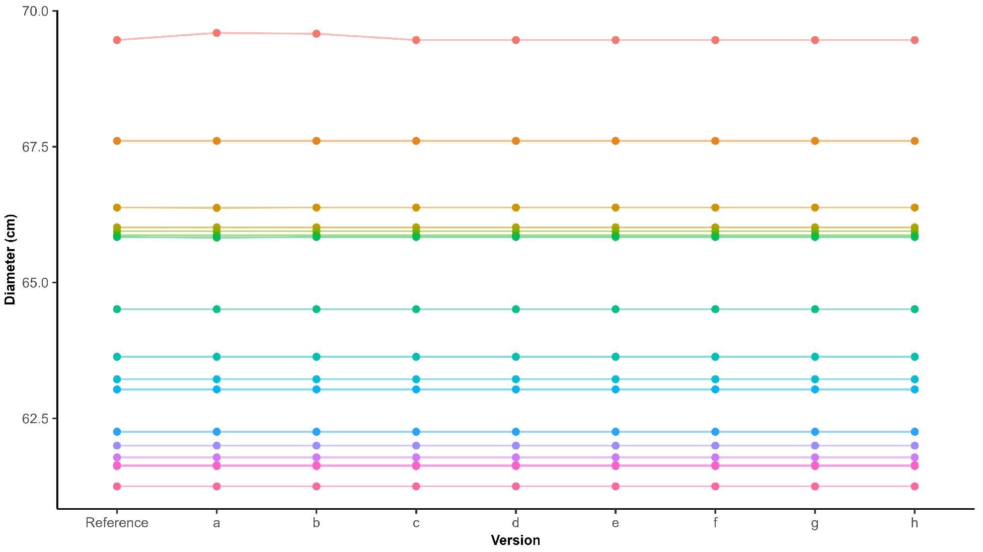
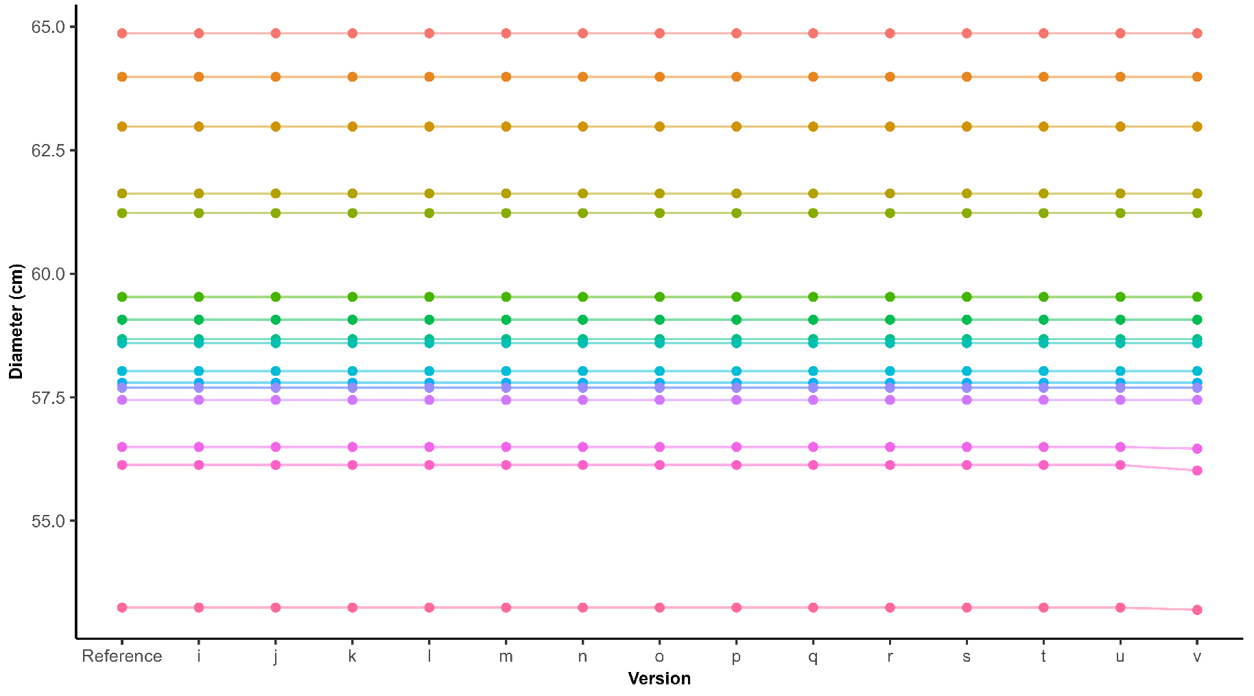
In summary, point prompt generation parameters affected the number of prompts and plants with masks but had minimal impact on the predicted diameter. If a mask was predicted, the IoU with the reference mask was often 1, indicating that mask shapes and estimated diameters remained consistent despite parameter changes, as illustrated in Figure A4. Variations in R 2 and MAE relative to the reference mainly reflect differences in sample size.
Figure A4. Effect of the values of the point prompts parameters, as described in Table A5, on the diameter estimations for 17 different plants. The diameter remained almost constant, suggesting that a similar segmentation mask was predicted even when parameters changed. The analysis is only displayed for plants where a mask was predicted for each version.
Horticulturae 11 01043 g0a4

Appendix B.3. Sensitivity Analysis of Post-Processing Parameters

Segmentation quality and the accuracy of diameter estimation were assessed for different values of the post-processing parameters. The results are reported in Figure A6.
The largest plant mask in the reference segmentation mask was 0.44 m2. When the maximum area was reduced to 1 or 2 times the IQR above the first quartile ( Q 1 ), such large masks were excluded, increasing false negatives and reducing recall. At 2 × IQR, recall remained stable within the evaluated regions, despite fewer masks compared to the reference. Similarly, setting the minimum area above the smallest reference mask (0.13 m2) led to the removal of smaller masks, resulting in a lower recall. However, it could improve precision by filtering out false positives. Adjusting the allowed area range by lowering the minimum area or raising the maximum area had limited impact. A small number of false positives, such as masks overlapping multiple plants or partially matching plant labels, occurred outside the evaluated regions.
Reducing the maximum eccentricity increased the required roundness for masks. As plants were not perfectly round, overly strict thresholds led to a sharp decline in recall. Allowing more elongated masks slightly increased the number of detected plant masks (10 across the full field for an eccentricity of 0.9, outside evaluated regions), but most overlapped multiple plants or only partially covered a single plant.
Similar to the effects observed when varying the point prompt generation parameters, modifying the post-processing settings influenced the amount of plants with a segmentation mask but did not alter the shape of the predicted masks or the diameter, as shown in Figure A5. As a result, the R 2 and MAE remained stable.
Figure A5. Effect of the values of the post-processing parameters, as mentioned in Table A6, on the diameter estimations for 17 different plants. The diameter remained almost constant, suggesting that a similar segmentation mask was predicted even when parameters changed. The analysis is only displayed for plants where a mask was predicted for each version.
Horticulturae 11 01043 g0a5

Appendix B.4. Impact of SAM 2.1 Encoder on Segmentation Accuracy and Diameter Estimation

The segmentation performance of the four different SAM 2.1 encoders, Hier-L, Hiera-B+, Hiera-S, and Hiera-T, is shown in Table A7. The smaller the encoder, the less plant masks were predicted, leading to lower recall. Missed plants often occurred in clusters. As demonstrated in Figure A6, masks were often less smooth, frequently extending beyond plant boundaries, especially for Hiera-S and Hiera-T, the two smallest models. These false positives contributed to lower precision and poorer diameter estimation. Despite the reported recall, visual inspection of the full segmented ROI from Hiera-B+ revealed more undetected plants compared to Hiera-L, suggesting a higher number of false negatives and an overestimation of recall. Although precision and diameter evaluation slightly improved, indicating closer resemblance to ground truth, the differences were minimal upon visual review.
Figure A6. Comparison of plant masks generated by different SAM 2.1 encoders.
Horticulturae 11 01043 g0a6
Table A4. Sensitivity analysis evaluating the impact of the DTM settings (number of elevation points and resolution) on segmentation quality and diameter estimation accuracy. Segmentation performance was evaluated for 480 plants, while diameter estimation was evaluated for the number of plants indicated in column “n”. The value for the minimum peak height was the same as described in Section 2.4 and is reported both as a quantile of all positive height values of the CHM (Q) and as an absolute value (in m) in the “Minimum peak height” column. The minimum distance in pixels was changed such that the distance in meters remained the same. Post-processing parameters maximum area, minimum area, and maximum eccentricity were held constant, as described in Section 2.6. The maximum area and minimum area are reported both as absolute values (in m2) and as scaled values: the maximum area was calculated by adding a multiple (x) of the IQR to Q 3 and the minimum area by subtracting a multiple (x) of the IQR from Q 1 . The first row presents the results for the parameter values used in the main analysis discussed in this article, hereafter referred to as reference. Evaluation outcomes that exceeded the reference are marked in green and those exhibiting inferior performance in red (comparison was performed up to two decimal digits). Parameter values highlighted in gray indicate the modified settings.
Point Prompt GenerationPost-ProcessingEvaluation Segmentation Mask After Post-ProcessingEvaluation Diameter
Elevation Points Resolution DTM (cm/px) Minimum Peak Height (Q|m) Maximum Area (x| m 2 ) Minimum Area (x| m 2 ) True Positives False Positives False Negatives Recall (%) Precision (%) F 1 (%) n R 2 MAE (cm)
5510.3|0.3563|0.473|0.124724499.1699.1699.161020.891.90
9 (GCPs)10.3|0.2563|0.47 *3|0.16 *46541197.6999.1598.4198 0.871.88
557.7 **0.3|0.3563|0.46 *3|0.12 *4714598.9599.1699.05101 0.881.89
5515.3 **0.3|0.3563|0.46 *3|0.12 *46731097.9099.3698.6399 0.851.91
** Given that the DSM had a resolution of 1.54 cm/px and the CHM adopted the lower resolution of the DSM and DTM, the resolution of the DTM directly determined the final resolution of the CHM. * As the CHM influenced the point prompt generation and this, in turn, influenced the segmentation results, the absolute values of the minimum and maximum area changed, although the relative values stayed the same. Diameter evaluation was performed only on plants that had a manual measurement and for which a predicted mask was available.
Table A5. Sensitivity analysis evaluating the impact of varying the minimum peak height and minimum distance between local maxima, two parameters of the point prompt generation (Section 2.4), on segmentation quality and diameter estimation accuracy. Segmentation performance was evaluated for 480 plants, while diameter estimation was evaluated for the number of plants indicated in column “n”. Minimum distance between local maxima is reported in both pixels and centimeters in the “Minimum distance” column. Minimum peak height is reported as a quantile of all positive height values of the CHM (Q) and as an absolute value (in m) in the “Minimum peak height” column. Post-processing parameters maximum area, minimum area, and maximum eccentricity were held constant, as described in Section 2.6. The maximum area and minimum area are reported both as absolute values (in m2) and as scaled values: the maximum area was calculated by adding a multiple (x) of the IQR to Q 3 and the minimum area by subtracting a multiple (x) of the IQR from Q 1 . The first row presents the results for the parameter values used in the main analysis discussed in this article, hereafter referred to as reference. Evaluation outcomes that exceeded the reference are marked in green, those equivalent to the reference are marked in orange and those exhibiting inferior performance are marked in red (comparison was performed up to two decimal digits). Parameter values highlighted in gray indicate the modified settings.
VersionPoint Prompt GenerationPost-ProcessingEvaluation Segmentation MaskEvaluation Diameter
Minimum Distance (px|m) Minimum Peak Height (q|m) Maximum Area (x| m 2 ) Minimum Area (x| m 2 ) True Positives False Positives False Negatives Recall (%) Precision (%) F 1 (%) n R 2 MAE (cm)
Reference10|0.1530.3|0.3563|0.473|0.124724499.1699.1699.16102 0.891.90
a1|0.0150.3|0.3563|0.47 *3|0.11 *4744299.5899.1699.37102 0.891.90
b5|0.0770.3|0.3563|0.47 *3|0.11 *4744299.5899.1699.37102 0.891.91
c15|0.2300.3|0.3563|0.46 *3|0.12 *45931896.2399.3597.76101 0.881.89
d20|0.3070.3|0.3563|0.46 *3|0.13 *41726187.2499.5292.9883 0.811.87
e10|0.1530.1|0.1383|0.47 *3|0.11 *4724499.1699.1699.16102 0.891.90
f10|0.1530.5|0.4233|0.47 *3|0.12 *45741996.0199.1397.5595 0.841.89
g10|0.1530.7|0.4733|0.47 *3|0.13 *39238582.1899.2489.9177 0.831.87
h10|0.1530.9|0.5333|0.48 *3|0.14 *164231434.3198.8050.9330 0.702.31
* As the parameters used for point prompt generation influenced the segmentation results, the absolute values of the minimum and maximum area changed, although the relative values stayed the same. Diameter evaluation was performed only on plants that had a manual measurement and for which a predicted mask was available.
Table A6. Sensitivity analysis evaluating the impact of varying the upper and lower threshold of the area (maximum area and minimum area) and the upper threshold for the eccentricity (maximum eccentricity), three parameters of the post-processing (Section 2.6), on segmentation quality and diameter estimation accuracy. Segmentation performance was evaluated for 480 plants, while diameter estimation was evaluated for the number of plants indicated in column “n”. Since the parameter values of the point prompt generation were held constant, the same point prompts were used as described in Section 2.4. Post-processing parameters maximum area and minimum area are reported both as absolute values (in m2) and as scaled values: the maximum area was calculated by adding a multiple (x) of the IQR to Q 3 and the minimum area by subtracting a multiple (x) of the IQR from Q 1 . The first row presents the results for the parameter values used in the main analysis discussed in this article, hereafter referred to as reference. Evaluation outcomes that exceeded the reference are marked in green, those equivalent to the reference in orange, and those exhibiting inferior performance in red (comparison was performed up to two decimal digits). Parameter values highlighted in gray indicate the modified settings.
VersionPost-ProcessingEvaluation Segmentation MaskEvaluation Diameter
Maximum Area (x| m 2 ) Minimum Area (x| m 2 ) Maximum Eccentricity True Positives False Positives False Negatives Recall (%) Precision (%) F 1 (%) n R 2 MAE (cm)
Reference3|0.473|0.120.754724499.1699.1699.16102 0.891.90
i1|0.363|0.120.7546641097.9099.1598.52100 0.891.89
j2|0.423|0.120.754724499.1699.1699.16102 0.891.90
k4|0.523|0.120.754724499.1699.1699.16102 0.891.90
l5|0.573|0.120.754724499.1699.1699.16102 0.891.90
m6|0.613|0.120.754724499.1699.1699.16102 0.891.90
n9|0.773|0.120.754724499.1699.1699.16102 0.891.90
o100|0.773|0.120.754724499.1699.1699.16102 0.891.90
p3|0.471|0.220.7545132694.5599.3496.8992 0.801.89
q3|0.472|0.170.7546531297.4899.3698.4198 0.841.89
r3|0.474|0.060.754724499.1699.1699.16102 0.891.90
s3|0.475|0.010.754724499.1699.1699.16102 0.891.90
t3|0.473|0.120.3069041114.38100.0025.1419 0.882.15
u3|0.473|0.120.6045722195.6199.5697.5599 0.891.90
v3|0.473|0.120.904724499.1699.1699.16102 0.891.90
Diameter evaluation was performed only on plants that had a manual measurement and for which a predicted mask was available.
Table A7. Evaluation of the segmentation performance across different SAM 2.1 encoders and their impact on diameter estimation. Segmentation performance was evaluated for 480 plants, while diameter estimation was evaluated for the number of plants indicated in column “n”. All segmentations were generated using the same point prompts, as described in Section 2.4. Post-processing was carried out using the parameter values mentioned in Section 2.6. Post-processing parameters maximum area and minimum area are reported both as absolute values (in m2) and as scaled values: the maximum area was calculated by adding a multiple (x) of the IQR to Q 3 and the minimum area by subtracting a multiple (x) of the IQR from Q 1 . The first row in the table presents the results for the SAM 2.1 encoder employed in the main analysis, hereafter referred to as the reference. Evaluation outcomes that outperformed the reference are marked in green, those equivalent in orange, and those with lower performance in red (comparison was performed up to two decimal digits).
SAM 2.1Post-ProcessingEvaluation Segmentation MaskEvaluation Diameter
Encoder Maximum Area (x| m 2 ) Minimum Area (x| m 2 ) True Positives False Positives False Negatives Recall (%) Precision (%) F 1 (%) n R 2 MAE (cm)
Hiera-L3|0.473|0.124724499.1699.1699.16102 0.891.90
Hiera-B+3|0.48 *3|0.11 *4762299.5899.5899.58102 0.891.85
Hiera-S3|0.49 *3|0.098 *4657898.3198.5298.41101 0.891.91
Hiera-T3|0.54 *3|0.06 *46461097.8998.7298.3198 0.891.94
* As the parameters used for point prompt generation influenced the segmentation results, the absolute values of the minimum and maximum area changed, although the relative values stayed the same. Diameter evaluation was performed only on plants that had a manual measurement and for which a predicted mask was available.

References

  1. Lamm, K.; Powell, A.; Lombardini, L. Identifying Critical Issues in the Horticulture Industry: A Delphi Analysis during the COVID-19 Pandemic. Horticulturae 2021, 7, 416. [Google Scholar] [CrossRef]
  2. Xu, X. Major challenges facing the commercial horticulture. Front. Hortic. 2022, 1, 980159. [Google Scholar] [CrossRef]
  3. Zhang, M.; Han, Y.; Li, D.; Xu, S.; Huang, Y. Smart horticulture as an emerging interdisciplinary field combining novel solutions: Past development, current challenges, and future perspectives. Hortic. Plant J. 2024, 10, 1257–1273. [Google Scholar] [CrossRef]
  4. Poenaru, M.M.; Manta, L.F.; Gherțescu, C.; Manta, A.G. Shaping the Future of Horticulture: Innovative Technologies, Artificial Intelligence, and Robotic Automation Through a Bibliometric Lens. Horticulturae 2025, 11, 449. [Google Scholar] [CrossRef]
  5. Sam, S.; Mira, L.; Kai, S. The impact of digitalization and automation on horticultural employees—A systematic literature review and field study. J. Rural. Stud. 2022, 95, 560–569. [Google Scholar] [CrossRef]
  6. Mahmud, M.S.; Zahid, A.; Das, A.K. Sensing and Automation Technologies for Ornamental Nursery Crop Production: Current Status and Future Prospects. Sensors 2023, 23, 1818. [Google Scholar] [CrossRef] [PubMed]
  7. Torres Gil, L.K.; Valdelamar Martínez, D.; Saba, M. The Widespread Use of Remote Sensing in Asbestos, Vegetation, Oil and Gas, and Geology Applications. Atmosphere 2023, 14, 172. [Google Scholar] [CrossRef]
  8. Hemeda, S. Applications of Remote Sensing; IntechOpen: London, UK, 2023. [Google Scholar]
  9. Toth, C.; Jóźków, G. Remote sensing platforms and sensors: A survey. ISPRS J. Photogramm. Remote Sens. 2016, 115, 22–36. [Google Scholar] [CrossRef]
  10. Yang, W.; Zhai, R. What can aerial phenotyping do and bring to us (breeders)? New Phytol. 2022, 236, 1584–1604. [Google Scholar] [CrossRef]
  11. Gill, T.; Gill, S.K.; Saini, D.K.; Chopra, Y.; de Koff, J.P.; Sandhu, K.S. A Comprehensive Review of High Throughput Phenotyping and Machine Learning for Plant Stress Phenotyping. Phenomics 2022, 2, 156–183. [Google Scholar] [CrossRef]
  12. Rayamajhi, A.; Jahanifar, H.; Mahmud, M.S. Measuring ornamental tree canopy attributes for precision spraying using drone technology and self-supervised segmentation. Comput. Electron. Agric. 2024, 225, 109359. [Google Scholar] [CrossRef]
  13. Abebe, A.M.; Kim, Y.; Kim, J.; Kim, S.L.; Baek, J. Image-Based High-Throughput Phenotyping in Horticultural Crops. Plants 2023, 12, 2061. [Google Scholar] [CrossRef] [PubMed]
  14. Argyrou, A.; Agapiou, A. A Review of Artificial Intelligence and Remote Sensing for Archaeological Research. Remote Sens. 2022, 14, 6000. [Google Scholar] [CrossRef]
  15. van der Meer, F.D.; van der Werff, H.M.A.; van Ruitenbeek, F.J.A.; Hecker, C.A.; Bakker, W.H.; Noomen, M.F.; van der Meijde, M.; Carranza, E.J.M.; Smeth, J.B.d.; Woldai, T. Multi- and hyperspectral geologic remote sensing: A review. Int. J. Appl. Earth Obs. Geoinf. 2012, 14, 112–128. [Google Scholar] [CrossRef]
  16. Sun, Z.; Wang, X.; Wang, Z.; Yang, L.; Xie, Y.; Huang, Y. UAVs as remote sensing platforms in plant ecology: Review of applications and challenges. J. Plant Ecol. 2021, 14, 1003–1023. [Google Scholar] [CrossRef]
  17. Khanal, S.; Kc, K.; Fulton, J.P.; Shearer, S.; Ozkan, E. Remote Sensing in Agriculture—Accomplishments, Limitations, and Opportunities. Remote Sens. 2020, 12, 3783. [Google Scholar] [CrossRef]
  18. Rai, R.K.; Karada, M.S.; Mishra, R.; Agnihotri, D.; Patel, K.K.; Thakur, S.; Singh, D. Transformative Role of Remote Sensing in Advancing Horticulture: Optimizing Sustainability, Efficiency and Resilience. Int. J. Environ. Clim. Change 2023, 13, 3559–3567. [Google Scholar] [CrossRef]
  19. Sishodia, R.P.; Ray, R.L.; Singh, S.K. Applications of Remote Sensing in Precision Agriculture: A Review. Remote Sens. 2020, 12, 3136. [Google Scholar] [CrossRef]
  20. Meraj, T.; Sharif, M.I.; Raza, M.; Alabrah, A.; Kadry, S.; Gandomi, A.H. Computer vision-based plants phenotyping: A comprehensive survey. iScience 2024, 27, 108709. [Google Scholar] [CrossRef]
  21. Araus, J.L.; Kefauver, S.C.; Vergara-Díaz, O.; Gracia-Romero, A.; Rezzouk, F.Z.; Segarra, J.; Buchaillot, M.L.; Chang-Espino, M.; Vatter, T.; Sanchez-Bragado, R.; et al. Crop phenotyping in a context of global change: What to measure and how to do it. J. Integr. Plant Biol. 2022, 64, 592–618. [Google Scholar] [CrossRef]
  22. Borra-Serrano, I.; Van Laere, K.; Lootens, P.; Leus, L. Breeding and Selection of Nursery Plants Assisted by High-Throughput Field Phenotyping Using UAV Imagery: Case Studies with Sweet Box (Sarcococca) and Garden Rose (Rosa). Horticulturae 2022, 8, 1186. [Google Scholar] [CrossRef]
  23. Yu, Y.; Wang, C.; Fu, Q.; Kou, R.; Huang, F.; Yang, B.; Yang, T.; Gao, M. Techniques and Challenges of Image Segmentation: A Review. Electronics 2023, 12, 1199. [Google Scholar] [CrossRef]
  24. Cheng, J.; Deng, C.; Su, Y.; An, Z.; Wang, Q. Methods and datasets on semantic segmentation for Unmanned Aerial Vehicle remote sensing images: A review. ISPRS J. Photogramm. Remote Sens. 2024, 211, 1–34. [Google Scholar] [CrossRef]
  25. Plaksyvyi, A.; Skublewska-Paszkowska, M.; Powroźnik, P. A Comparative Analysis of Image Segmentation Using Classical and Deep Learning Approach. Adv. Sci. Technology. Res. J. 2023, 17, 127–139. [Google Scholar] [CrossRef]
  26. Zhang, J.; Lu, J.; Zhang, Q.; Qi, Q.; Zheng, G.; Chen, F.; Chen, S.; Zhang, F.; Fang, W.; Guan, Z. Estimation of Garden Chrysanthemum Crown Diameter Using Unmanned Aerial Vehicle (UAV)-Based RGB Imagery. Agronomy 2024, 14, 337. [Google Scholar] [CrossRef]
  27. Zheng, C.; Abd-Elrahman, A.; Whitaker, V.M.; Dalid, C. Deep Learning for Strawberry Canopy Delineation and Biomass Prediction from High-Resolution Images. Plant Phenomics 2022, 2022, 9850486. [Google Scholar] [CrossRef]
  28. Chadwick, A.J.; Goodbody, T.R.H.; Coops, N.C.; Hervieux, A.; Bater, C.W.; Martens, L.A.; White, B.; Röeser, D. Automatic Delineation and Height Measurement of Regenerating Conifer Crowns under Leaf-Off Conditions Using UAV Imagery. Remote Sens. 2020, 12, 4104. [Google Scholar] [CrossRef]
  29. Fu, H.; Zhao, H.; Jiang, J.; Zhang, Y.; Liu, G.; Xiao, W.; Du, S.; Guo, W.; Liu, X. Automatic detection tree crown and height using Mask R-CNN based on unmanned aerial vehicles images for biomass mapping. For. Ecol. Manag. 2024, 555, 121712. [Google Scholar] [CrossRef]
  30. Erdem, F.; Ocer, N.E.; Matci, D.K.; Kaplan, G.; Avdan, U. Apricot Tree Detection from UAV-Images Using Mask R-CNN and U-Net. Photogramm. Eng. Remote Sens. 2023, 89, 89–96. [Google Scholar] [CrossRef]
  31. Ye, Z.; Wei, J.; Lin, Y.; Guo, Q.; Zhang, J.; Zhang, H.; Deng, H.; Yang, K. Extraction of Olive Crown Based on UAV Visible Images and the U2-Net Deep Learning Model. Remote Sens. 2022, 14, 1523. [Google Scholar] [CrossRef]
  32. Ji, Y.; Yan, E.; Yin, X.; Song, Y.; Wei, W.; Mo, D. Automated extraction of Camellia oleifera crown using unmanned aerial vehicle visible images and the ResU-Net deep learning model. Front. Plant Sci. 2022, 13, 958940. [Google Scholar] [CrossRef] [PubMed]
  33. Mo, J.; Lan, Y.; Yang, D.; Wen, F.; Qiu, H.; Chen, X.; Deng, X. Deep Learning-Based Instance Segmentation Method of Litchi Canopy from UAV-Acquired Images. Remote Sens. 2021, 13, 3919. [Google Scholar] [CrossRef]
  34. Magistri, F.; Weyler, J.; Gogoll, D.; Lottes, P.; Behley, J.; Petrinic, N.; Stachniss, C. From one field to another—Unsupervised domain adaptation for semantic segmentation in agricultural robotics. Comput. Electron. Agric. 2023, 212, 108114. [Google Scholar] [CrossRef]
  35. Rafi, T.H.; Mahjabin, R.; Ghosh, E.; Ko, Y.W.; Lee, J.G. Domain generalization for semantic segmentation: A survey. Artif. Intell. Rev. 2024, 57, 247. [Google Scholar] [CrossRef]
  36. Potena, C.; Nardi, D.; Pretto, A. Fast and Accurate Crop and Weed Identification with Summarized Train Sets for Precision Agriculture. In Intelligent Autonomous Systems 14; Chen, W., Hosoda, K., Menegatti, E., Shimizu, M., Wang, H., Eds.; Springer: Cham, Switzerland, 2017; pp. 105–121. [Google Scholar] [CrossRef]
  37. Ravi, N.; Gabeur, V.; Hu, Y.T.; Hu, R.; Ryali, C.; Ma, T.; Khedr, H.; Rädle, R.; Rolland, C.; Gustafson, L.; et al. SAM 2: Segment Anything in Images and Videos. arXiv 2024, arXiv:2408.00714. Available online: http://arxiv.org/abs/2408.00714 (accessed on 28 October 2024).
  38. Gillies, S.; Ward, B.; Petersen, A.S. Rasterio: Geospatial Raster I/O for Python Programmers. 2013. Available online: https://github.com/mapbox/rasterio (accessed on 28 October 2024).
  39. Virtanen, P.; Gommers, R.; Oliphant, T.E.; Haberland, M.; Reddy, T.; Cournapeau, D.; Burovski, E.; Peterson, P.; Weckesser, W.; Bright, J.; et al. SciPy 1.0: Fundamental Algorithms for Scientific Computing in Python. Nat. Methods 2020, 17, 261–272. [Google Scholar] [CrossRef]
  40. Borra-Serrano, I.; De Swaef, T.; Muylle, H.; Nuyttens, D.; Vangeyte, J.; Mertens, K.; Saeys, W.; Somers, B.; Roldán-Ruiz, I.; Lootens, P. Canopy height measurements and non-destructive biomass estimation of Lolium perenne swards using UAV imagery. Grass Forage Sci. 2019, 74, 356–369. [Google Scholar] [CrossRef]
  41. Walt, S.v.d.; Schönberger, J.L.; Nunez-Iglesias, J.; Boulogne, F.; Warner, J.D.; Yager, N.; Gouillart, E.; Yu, T. scikit-image: Image processing in Python. PeerJ 2014, 2, e453. [Google Scholar] [CrossRef]
  42. Bradski, G. The OpenCV Library. Dr. Dobb’s J. Softw. Tools 2000. [Google Scholar]
  43. Gillies, S.; van der Wel, C.; Van den Bossche, J.; Taves, M.W.; Arnott, J.; Ward, B.C. Shapely, Version 2.0.7. 2025. Available online: https://zenodo.org/records/15463269 (accessed on 26 June 2025).
  44. QGIS Development Team. QGIS Geographic Information System; QGIS Association. Available online: https://www.qgis.org (accessed on 26 June 2025).
  45. Torres-Sánchez, J.; López-Granados, F.; Borra-Serrano, I.; Peña, J.M. Assessing UAV-collected image overlap influence on computation time and digital surface model accuracy in olive orchards. Precis. Agric. 2018, 19, 115–133. [Google Scholar] [CrossRef]
  46. Zhang, R.; Jiang, Z.; Guo, Z.; Yan, S.; Pan, J.; Ma, X.; Dong, H.; Gao, P.; Li, H. Personalize Segment Anything Model with One Shot. arXiv 2023, arXiv:2305.03048. Available online: http://arxiv.org/abs/2305.03048 (accessed on 26 June 2025).
  47. Osco, L.P.; Wu, Q.; de Lemos, E.L.; Gonçalves, W.N.; Ramos, A.P.M.; Li, J.; Marcato, J. The Segment Anything Model (SAM) for remote sensing applications: From zero to one shot. Int. J. Appl. Earth Obs. Geoinf. 2023, 124, 103540. [Google Scholar] [CrossRef]
  48. Vigneault, P.; Lafond-Lapalme, J.; Deshaies, A.; Khun, K.; de la Sablonnière, S.; Filion, M.; Longchamps, L.; Mimee, B. An integrated data-driven approach to monitor and estimate plant-scale growth using UAV. ISPRS Open J. Photogramm. Remote Sens. 2024, 11, 100052. [Google Scholar] [CrossRef]
Figure 1. High-level summary of the proposed pipeline, illustrating the major processing steps.
Horticulturae 11 01043 g001
Figure 2. Orthomosaic of the observed area of the chrysanthemum field, captured on October 15, together with the ROIs. ROI 1 is outlined in orange and ROI 2 is in blue.
Horticulturae 11 01043 g002
Figure 3. Location of the ground control points (GCPs) (light gray squares) used for georeferencing and the additional points (red rectangles) used to create the digital terrain model (DTM), visualized in the orthomosaic of each flight. The elevation data from the GCPs were also incorporated into the DTM. (A) Orthomosaic of the flight on 8 October at 11:03 a.m. over ROI 1. For georeferencing purposes, 5 GCPs were laid out across the field, and the DTM was derived from the elevation of 37 locations. (B) Flight on 8 October at 12:25 p.m. over ROI 2. A set of 5 GCPs was used for georeferencing and the DTM was created based on data from 30 points. (C) Flight on 15 October at 12:42 p.m. covering both ROI 1 and 2. Nine GCPs were used for georeferencing and the DTM was generated from the elevation of 55 locations.
Horticulturae 11 01043 g003
Figure 4. (A) Single 1024 x 1024 tile of the orthomosaic captured on October 15 at 12:42 p.m. (B) Prompts (white dots) corresponding with the top of the plants (local maxima in the CHM), indicating the objects to segment. (C) Combined mask of all individual plant segmentation masks within the tile, as predicted by Segment Anything Model 2.1 (SAM 2.1), overlaid on the orthomosaic. Distinct colors denote different plant masks. The white dots represent the point prompts, each of which triggered the prediction of a corresponding plant segmentation mask. (D) Plant segmentation masks preserved since they did not lie entirely within the 256-pixel-wide border. The masks are overlaid on the orthomosaic.
Horticulturae 11 01043 g004
Figure 5. Segmentation mask of a single object predicted by the segmentation model SAM 2.1, containing multiple connected regions. The region in the red box did not belong to the plant and was excluded.
Horticulturae 11 01043 g005
Figure 6. Part of the orthomosaic from ROI 2, captured on October 15, illustrating poor segmentation performance, with several chrysanthemums lacking a mask (white outline). The point prompts are visualized as white dots, indicating that poor segmentation was not due to the absence of a point prompt for the plant. SAM 2.1 appeared to struggle with segmenting chrysanthemums that lacked clear boundaries and exhibited a speckled pattern.
Horticulturae 11 01043 g006
Figure 11. Comparison between measured and predicted crown diameters (cm) of selected chrysanthemums from sections 1, 3, and 6 within ROI 2. Each point represents an individual plant measurement. (A) Measurements performed on the orthomosaic of 8 October. (B) Measurements performed on the orthomosaic of 15 October.
Horticulturae 11 01043 g011
Figure 12. Distribution of the predicted crown diameters (cm) for the chrysanthemums in ROI 2 on 8 October (A) and 15 October 2024 (B).
Horticulturae 11 01043 g012
Table 1. Area and number of plants per region of interest (ROI) on the two observation dates.
ROIDateArea ( m 2 )Number of Plants
18 October 202432908131
15 October 202432908131
28 October 202428687278
15 October 202428687275
Table 2. Resolution of the digital surface model (DSM), the DTM, and the canopy height model (CHM).
DateTimeResolution of the DSM ( cm / px )Resolution of the DTM ( cm / px )Resolution of the CHM ( cm / px )
8 October 202411:03 a.m.1.481.00 *1.48
8 October 202412:25 p.m.1.491.00 *1.49
15 October 202412:42 p.m.1.541.00 *1.54
* The resolution of the DTM reflects the chosen resolution of the underlying interpolation grid.
Table 3. Evaluation of the field-level segmentation mask for each ROI per flight date. True positives were masks with a visually estimated intersection over union (IoU) of at least 0.8. False positives included masks with an IoU below 0.8 or masks that did not correspond to any chrysanthemum. False negatives represented chrysanthemums that were not segmented. False positives and false negatives were manually counted. The number of true positives was calculated as the difference between the total number of masks and the false positives.
ROIDateTrue PositivesFalse PositivesFalse NegativesRecallPrecision F 1
18 October 202479741115798.0799.8698.96
15 October 20247955017697.84100.098.91
28 October 20246979129995.8999.9997.90
15 October 20246938033795.37100.0097.63
allall298461296996.8699.9698.38
Disclaimer/Publisher’s Note: The statements, opinions and data contained in all publications are solely those of the individual author(s) and contributor(s) and not of MDPI and/or the editor(s). MDPI and/or the editor(s) disclaim responsibility for any injury to people or property resulting from any ideas, methods, instructions or products referred to in the content.