Segmentation-Based Classification of Plants Robust to Various Environmental Factors in South Korea with Self-Collected Database

Abstract

Many plant image-based studies primarily use datasets featuring either a single plant, a plant with only one leaf, or images containing only plants and leaves without any background. However, in real-world scenarios, a substantial portion of acquired images consists of blurred plants or extensive backgrounds rather than high-resolution details of the target plants. In such cases, classification models struggle to identify relevant areas for classification, leading to insufficient information and reduced classification performance. Moreover, the presence of moisture, water droplets, dust, or partially damaged leaves further degrades classification accuracy. To address these challenges and enhance classification performance, this study introduces a plant image segmentation (Pl-ImS) model for segmentation and a plant image classification (Pl-ImC) model for classification. The proposed models were evaluated using a self-collected dataset of 21,760 plant images captured under real field conditions in South Korea, incorporating various environmental factors such as moisture, water droplets, dust, and partial leaf loss. The segmentation method achieved a dice score (DS) of 89.90% and an intersection over union (IoU) of 81.82%, while the classification method attained an F1-score of 95.97%, surpassing state-of-the-art methods.

1. Introduction

Various systems incorporating cameras and artificial intelligence (AI) algorithms have been developed for the segmentation and classification of plant images. These systems are extensively applied in multiple domains, including crop disease classification and detection [1,2,3], plant disease diagnosis [4], fruit classification [5,6,7,8], and plant classification [9,10,11,12]. For plant recognition using images acquired by camera devices, several approaches exist, including detection algorithms [3], image blur removal techniques [13], hand-crafted algorithms, and methods utilizing image datasets that have been manually processed [14].

Previous studies have used images with only a single plant leaf [15,16], images with only a single plant [17], and images full of plants and plant leaves with little background [18]. Moreover, in datasets consisting entirely of plants and leaves without a background, many images feature blurred plant regions rather than high-resolution details of the target plant (Figure 1h). Furthermore, in datasets containing a single plant or a plant with only one leaf, most images include more background than plant content, or only a partial leaf is visible (Figure 1e–g). In such cases, classification models struggle to identify the relevant regions for classification, leading to insufficient information for plant image classification and a decline in performance. Additionally, classification accuracy may further deteriorate when plants are covered with moisture, water droplets, or dust (Figure 2) or when a leaf is partially lost (Figure 3).

Figure 1a–d present standard images primarily featuring intact plant leaves. Figure 1e contains numerous high-quality small fragments of leaves and plant stems. Figure 1f includes high-quality small leaf fragments along with background elements such as other plants. Figure 1g features a high-quality portion of leaves but also includes blurred and dark plant content. Figure 1h shows a high-quality portion of leaves alongside blurred plant content. Since most of these images lack crucial high-resolution details, they contribute to a decline in plant recognition performance.

Figure 3 depicts plant leaves that have been partially damaged by insects. Despite the impact of such issues, previous studies have largely overlooked them, leading to a significant decline in plant image classification accuracy when these conditions occur. To address these challenges, this study conducted various experiments and proposed a plant image segmentation (Pl-ImS) model and a plant image classification (Pl-ImC) model to enhance classification performance. The segmentation network incorporates residual and dense blocks and is trained using the generative adversarial network (GAN) concept [20]. The images generated by the segmentation network undergo a masking operation before being processed by the classification network. Experiments were conducted using the self-collected dataset, which includes the issues highlighted in Figure 1, Figure 2 and Figure 3. Since existing open datasets do not account for these issues, they were not utilized in this study. To evaluate segmentation performance and compare it with existing approaches, ResNet-50 [21] was used for classification in each method. Furthermore, the Pl-ImC network incorporates residual and dense blocks, similar to the Pl-ImS network. During model development, the architecture and hyperparameters were carefully tuned throughout training to effectively handle the various cases presented in Figure 1, Figure 2 and Figure 3.

Theoretical knowledge of Pl-ImS: Residual networks enable the construction of deeper networks by introducing identity skip-connections that alleviate the vanishing gradient problem. These residual connections allow gradients to flow directly through shortcut paths, enabling stable and efficient training of very deep networks.

Dense Nets further enhance feature propagation by connecting each layer to all subsequent layers within a block. This design promotes feature reuse and efficient gradient flow, reducing redundancy while increasing representational capacity. In our segmentation model, we integrate both concepts through a custom-designed residual dense (Dense) block, combining residual shortcuts with densely connected layers to perform multi-scale feature fusion, which is essential for segmenting only the high-quality, informative regions of plant leaves from noisy backgrounds.

To further refine segmentation outputs, the architecture is trained within a GAN framework. GANs operate through adversarial training between a generator and a discriminator, where the discriminator guides the generator to produce more realistic outputs. This mechanism is theoretically supported by minimax optimization and distribution matching, enabling the segmentation model to generate sharper, more accurate boundary predictions by emphasizing high-quality leaf regions during training.

Theoretical knowledge of Pl-ImC: The classification stage requires robust extraction of discriminative features from the segmented leaf regions. We adopt a lightweight residual architecture, as residual blocks are known to preserve important feature hierarchies while allowing deeper representations without degradation in performance. Residual learning not only accelerates convergence but also enhances generalization, especially when data quality or quantity is limited.

Unlike the segmentation task, where detailed spatial structure is crucial, classification benefits more from global abstraction and semantic compression. Therefore, our classification model uses only residual blocks with carefully selected convolutional layers to maintain sufficient depth and receptive field while significantly reducing the number of parameters. This minimal yet effective design supports fast inference and deployability on edge or mobile devices without sacrificing accuracy.

Our main contributions in this study are explained in the following:

-

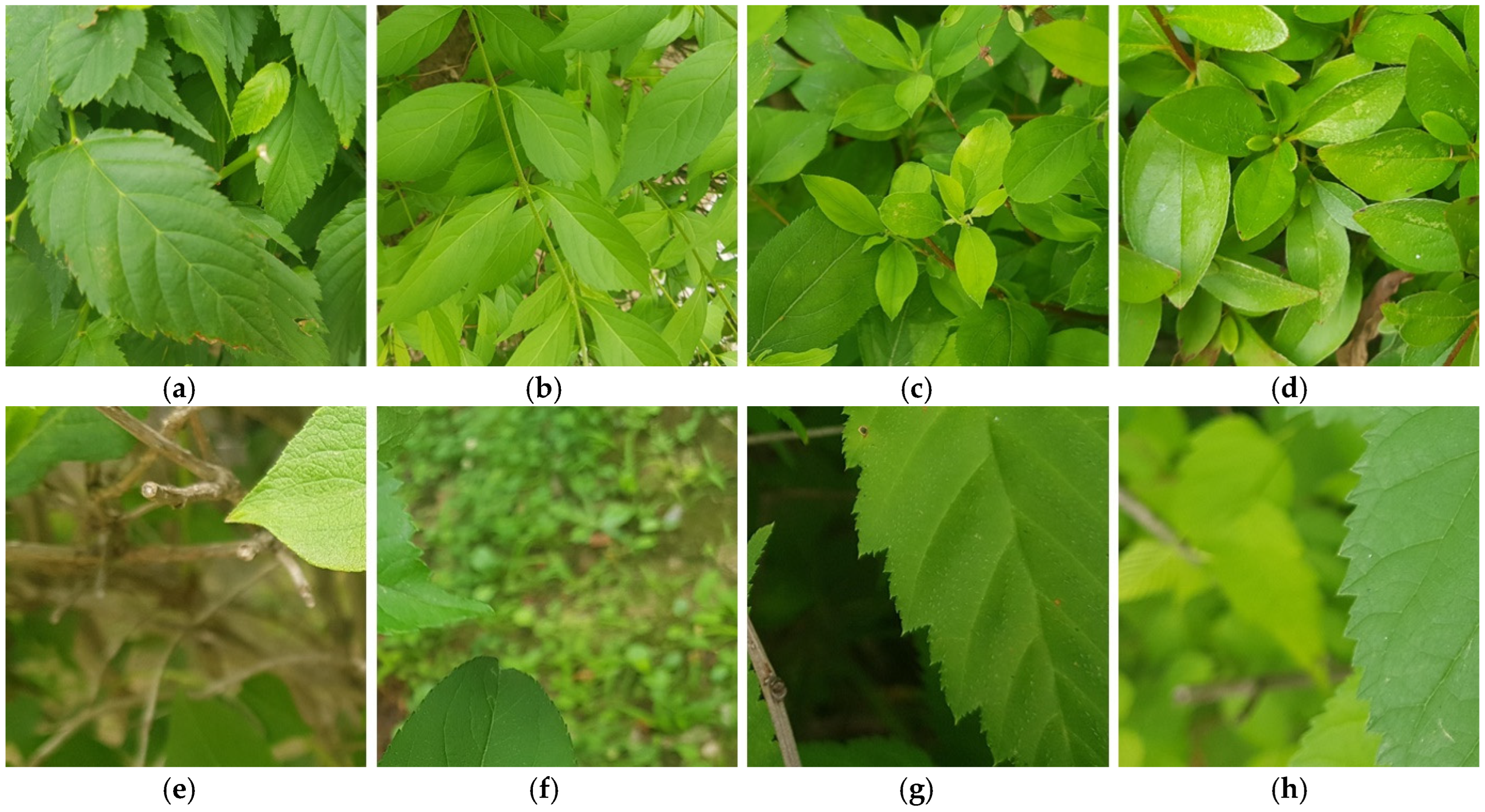
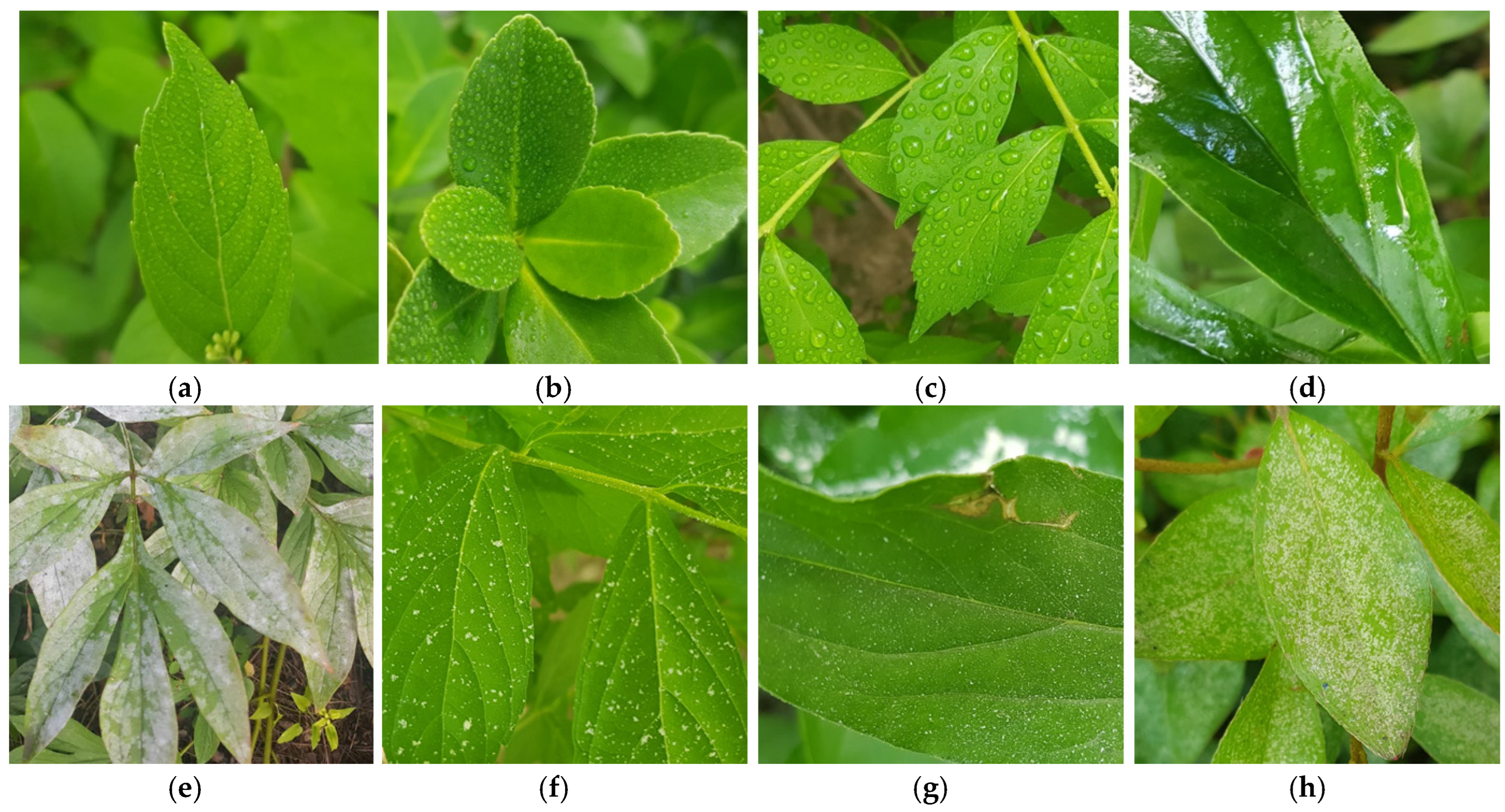
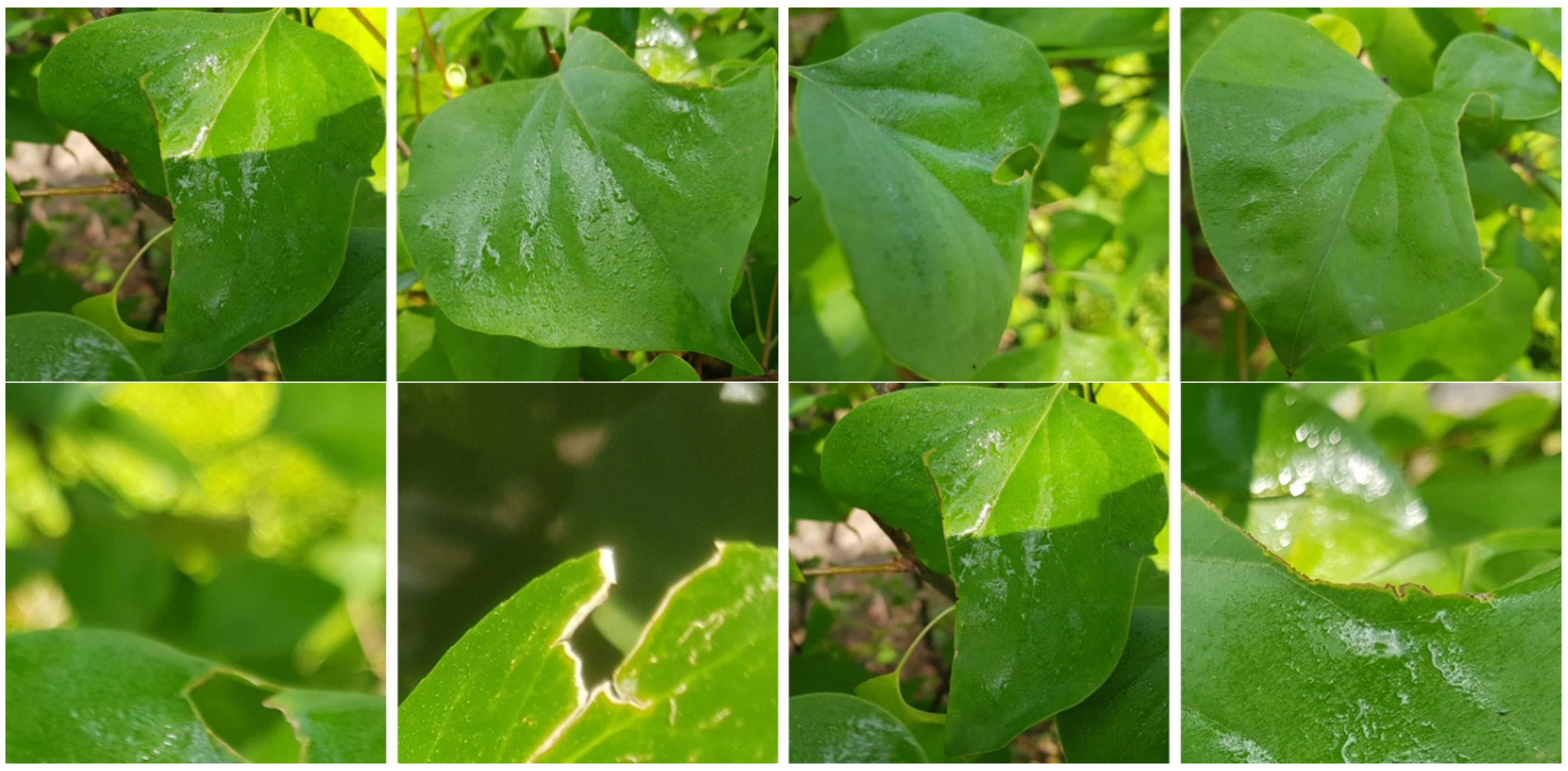
When capturing close-up images of plant leaves, the camera’s shallow depth of field (DoF) often results in only a portion of the leaf being in focus, while the rest appears blurred. Typically, the focused area is considered the primary region of interest for recognition. However, most previous studies have not addressed this issue. This study explores plant recognition by focusing on clearly visible leaf regions and disregarding blurred areas. Furthermore, while previous studies did not consider input images containing moisture, water droplets, dust, or partially missing leaves, this study collects and investigates a dataset of plant images captured in real field environments with complex backgrounds in South Korea.

-

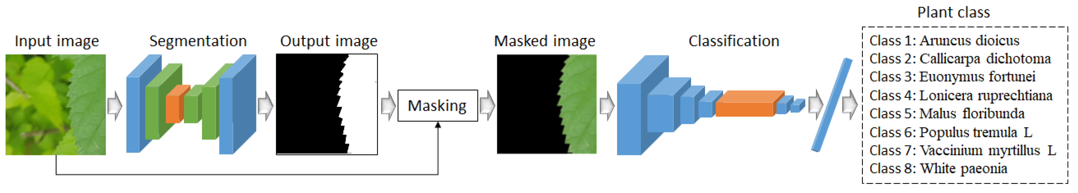
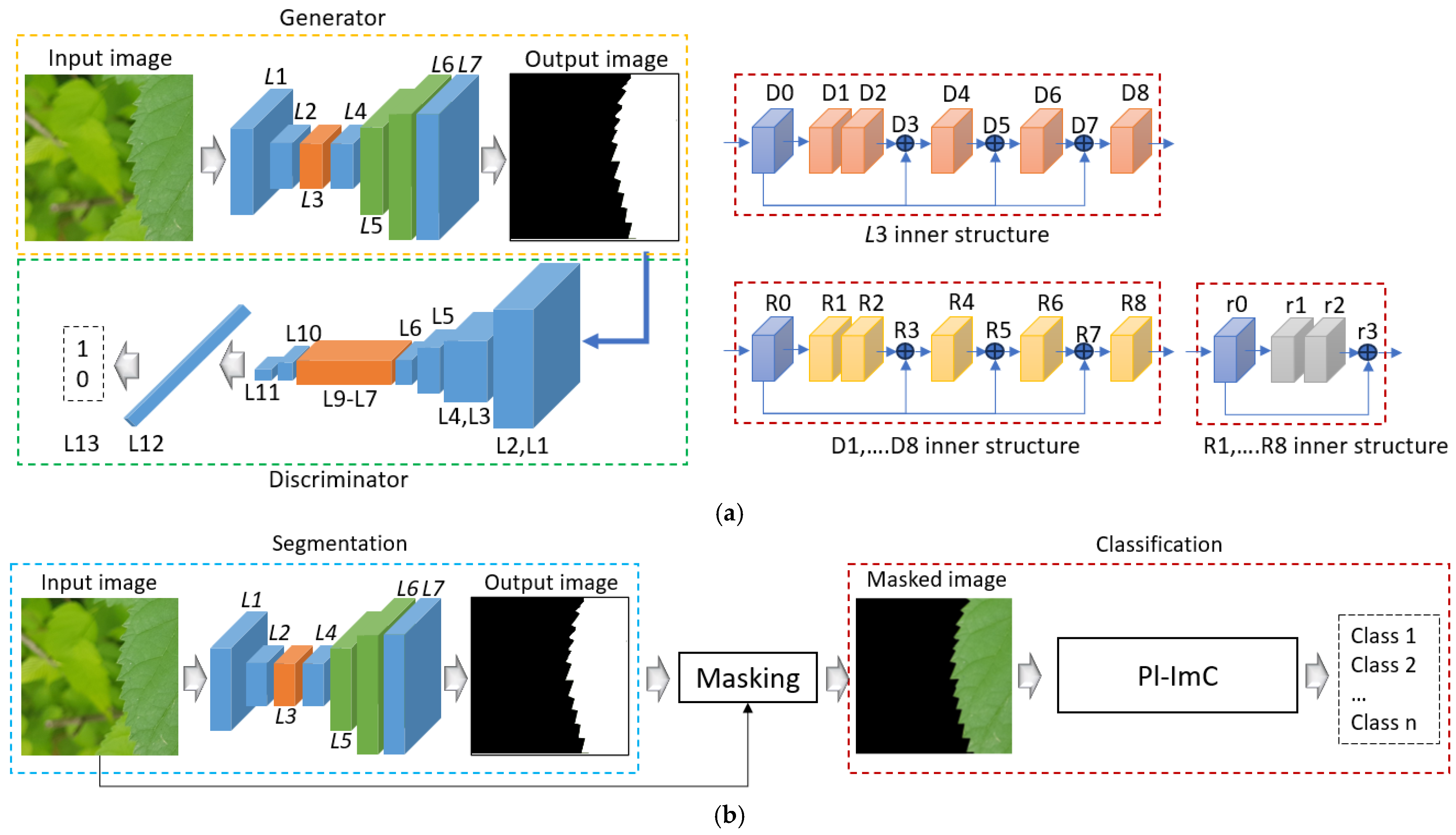
To address these challenges, this study proposes the Pl-ImS network in plant image segmentation. The Pl-ImS network incorporates residual blocks and a densely connected architecture, optimized based on the self-collected dataset. Additionally, a new residual DenseNet (RDense) block is designed, integrating five densely connected blocks. The RDense block architecture enables skip-connection-based feature fusion at multiple steps, ensuring high segmentation performance. Moreover, the Pl-ImS network is trained using a GAN framework, incorporating a discriminator network to improve performance. During training, ground-truth images are prepared to facilitate segmentation, emphasizing only the high-quality plant regions in the input images.

-

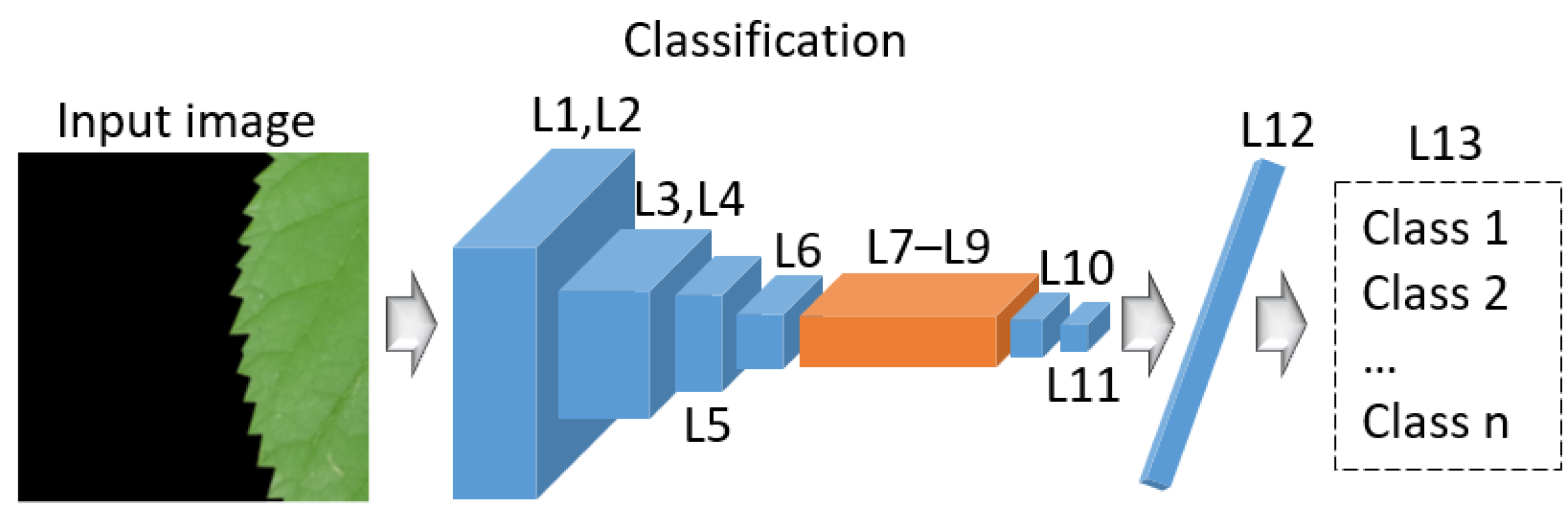
To further improve classification performance, this study proposes the Pl-ImC network in plant image classification. In the Pl-ImC network, using only residual blocks yields better performance than incorporating a densely connected network. Therefore, the architecture is designed with three residual blocks and eight convolutional layers. Since the Pl-ImS network has a large number of parameters and a slow processing speed, a simplified architecture is implemented for the Pl-ImC network, reducing the number of parameters to 2.1 M to enhance processing efficiency. Additionally, overall model design time is minimized by utilizing only the simplified fully connected (FC) layer architecture from the Pl-ImC network as the discriminator network for the Pl-ImS network.

-

Fractal dimension estimation is applied to the Pl-ImS network to further refine segmentation performance. Moreover, the proposed models, source codes, and built databases are available on GitHub [19].

The rest of the paper is organized as follows. Section 2 provides an in-depth discussion of previous plant-related studies. Section 3 details the proposed methods. Section 4 presents all experimental results and relevant analyses. Section 5 discusses the results. Section 6 concludes the study.

2. Related Work

In this section a comprehensive review of existing studies on plant image segmentation and classification is presented. The existing research can be categorized into two areas: plant image segmentation studies and plant image classification studies.

2.1. Plant Image Segmentation Studies

This subsection reviews previous studies on plant image segmentation, divided into two groups: studies that used images featuring a single plant, such as a single leaf, fruit, or vegetable, and studies that analyzed images containing multiple plants, including multiple leaves, fruits, or vegetables.

2.1.1. Images with a Single Plant

Yang et al. [22] employed the tree dataset of urban street (TDUS) and introduced a leaf detection based on YOLOv8 to avoid background interference during the stage 2 leaf segmentation process. They then proposed an enhanced DeepLabv3+-based leaf segmentation method to efficiently detect stick leaves and thin petioles. Similarly, Shoaib et al. [23] used the PlantVillage dataset [15] and proposed a deep learning-based system for detecting tomato plant diseases using a plant leaf dataset.

2.1.2. Images with Multiple Plants

Wang et al. [17] employed computer vision problems in the plant phenotyping (CVPPP) dataset and implemented a YOLOv8-seg model for leaf segmentation. To enhance segmentation performance, they proposed a bidirectional feature pyramid network (BiFPN) module and a ghost module for the standard YOLOv8, resulting in two improved versions. Ward et al. [24] proposed a method of leaf segmentation using an augmentation method on real plant datasets with composite plant images generated through domain randomization. They also trained a state-of-the-art (SOTA) deep learning segmentation model, Mask R-CNN [25], using a combination of real and synthetic Arabidopsis plant images from the CVPPP dataset. Milioto et al. [26] used three distinct plant image datasets, Bonn, Stuttgart, and Zurich, collected from Germany and Switzerland. Their study tackled the challenge of distinguishing beet plants, weeds, and background using a convolutional neural network-based semantic segmentation (CNN-SS) approach and an RGB dataset. Additionally, they proposed a CNN capable of real-time classification using existing vegetation indices and deployed the system on agricultural robots operating across various fields in Germany and Switzerland, thoroughly evaluating its performance.

2.2. Plant Image Classification Studies

This subsection reviews previous studies on plant image classification, categorizing them into three groups: those using images of a single plant, those utilizing images with multiple plants, and those incorporating both types of datasets.

2.2.1. Images with a Single Plant

Hamid et al. [27] performed an experiment on classification by using an existing CNN, AlexNet, and a bag of features (BoF), comparing their performance on the Fruits-360 [16] dataset. Katarzyna et al. [28] also used a CNN and the Fruits-360 dataset. Moreover, YOLO-V3 was used for extracting regions of interest (ROI) from the original images of apples to perform classification. Siddiqi [29] proposed FruitNet and compared fourteen deep learning-based methods on the Fruits-360 dataset to assess classification performance. Kader et al. [6] performed fruit recognition experiments on the Fruits-360 dataset and performed a comparative analysis of different types of machine learning-based techniques that included support vector machines (SVM), linear discriminant analysis, Naïve Bayes, random forests, decision trees, k-nearest neighbors, and logistic regression. Additionally, the study applied different feature extraction methods, including color histograms, Hu moments, and Haralick texture, to enhance classification performance.

2.2.2. Images with Multiple Plants

Abawatew et al. [9], Ashwinkumar et al. [10], and Chakraborty et al. [11] proposed classification methods based on the attention-augmented residual (AAR) network, optimal mobile network-based convolutional neural networks (OMNCNN), and DenseNet-121 [30], respectively, conducting experiments on classification using the PlantDoc database [18]. Chompookham et al. [31] evaluated five network types, Xception, MobileNetV1, NASNetMobile, MobileNetV2, and DenseNet-121, on the same dataset. Anasta et al. [2] performed an experiment on their own newly collected dataset to detect disease-affected regions in visible light images based on thermal imaging and if-then rules. However, the manual observation and analysis of these detected regions proved to be a time-consuming process. Batchuluun et al. [32] developed a network named the plant classification residual (PlantCR), which simultaneously processes thermal and visual images for multi-class classification by integrating features extracted from both image types. Raza et al. [3] presented thermal and visual image-based approaches to conduct experiments on a binary classification, utilizing three different camera devices for capturing visual and thermal images. By integrating the three images, classification accuracy for distinguishing healthy and diseased plants was enhanced. Additionally, manually extracted features, analysis of variance (ANOVA) [33], and SVM were utilized to conduct a binary classification. Batchuluun et al. [34] enhanced classification performance by employing a network named the plant super-resolution (PlantSR) for upscaling images before inputting them into a classification network named the plant multi-class classification (PlantMC), utilizing both visible light and thermal images. These studies relied on self-collected datasets to validate their approaches.

2.2.3. Images with Single and Multiple Plants

Wang et al. [12] introduced a trilinear convolutional neural network (T-CNN) for a plant image classification task and used the PlantDoc and PlantVillage open datasets. Biswas et al. [7] introduced a multi-class CNN and tested the model using the FIDS30 and Fruits-360 datasets. Shahi et al. [5] proposed a deep learning method for attention-based fruit classification, utilizing pre-trained models named ImageNet and MobileNetV2, and compiled three fruit-related datasets. Hossain et al. [8] conducted classification experiments using CNN, VGG-16, a CNN-based lightweight model, pre-trained models, and datasets generated from a supermarket and self-collected sources.

However, a limitation of these previous studies is that they did not consider real field conditions, such as the presence of moisture, water droplets, dust on plant surfaces, or the partial loss of leaves. Moreover, these studies primarily used image datasets featuring plant leaves against a clean background, making their methods difficult to apply in real field environments. Another overlooked aspect was the presence of blurred areas in plant images, which affects classification accuracy (Figure 1h). To address the limitations above, a self-collected database that accounts for real field conditions and proposes the Pl-ImS and Pl-ImC models was created in this study.

Table 1. Comparison of our and previous plant image-based studies.

Task	Type	Dataset	Method		Advantage	Disadvantage
Segmentation	Single plant	TDUS	DEEPLABV3+ [22]		- Considers images from real field conditions - Effective for segmenting a single plant in images	- Fails to account for various environmental factors (missing parts of the plant’s leaves due to blurring, the presence of small or large water droplets, dust, or insects) and cannot segment multiple plants at once
		PlantVillage	Modified U-Net [23]		- Can segment both plant parts and disease-affected areas - Effective for segmenting a single plant in images	- Does not consider images captured in real farmland environment - Fails to account for various environmental factors (missing parts of the plant’s leaves due to blurring, the presence of small or large water droplets, dust, or insects) and cannot segment multiple plants at once
	Multiple plants	CVPPP	YOLOv8-seg [17] Mask-RCNN [24]		Able to segment multiple plant leaves simultaneously	- Simultaneously segmenting multiple plants is time-consuming and less accurate - Fails to consider various factors (missing parts of the plant’s leaves due to blurring, the presence of small or large water droplets, dust, or insects)
		Bonn, Stuttgart, and Zurich	CNN-SS [26]		- Considers various illumination conditions and soil types - Considers images from real field conditions - Able to segment multiple plants simultaneously	- Images become blurred as robots move while capturing images in farms - Simultaneously segmenting multiple plants is time-consuming and less accurate - Fails to consider various factors (missing parts of the plant’s leaves due to blurring, the presence of small or large water droplets, dust, or insects)
Classification	Single plant	Fruits-360	Alexnet [27]; YOLO-V3 [28]; FruitNet [29]; SVM [6]		It is effective to segment a single plant in images.	- Reduced performance when images contain multiple plants or a large background - Does not consider images captured in a real farmland environment - Fails to consider various factors (missing parts of the plant’s leaves due to blurring, the presence of small or large water droplets, dust, or insects)
	Single and multiple plants	FIDS30 and Fruits-360	CNN-based [7]		- Consistent performance regardless of the number of plants - Considers various scenarios, including images with a single plant or a large background, filled with plant content, etc.	Fails to account for various environmental factors (missing parts of the plant’s leaves due to blurring, the presence of small or large water droplets, dust, or insects)
		Supermarket produce, self-collected	VGG16-based [8]		- Segmenting various plant images acquired from supermarkets effectively - Consistent performance regardless of the number of plants	- Does not consider images captured in a real farmland environment - Fails to consider various factors (missing parts of the plant’s leaves due to blurring, the presence of small or large water droplets, dust, or insects)
		Dataset collection	MobileNetV2 [5]		- Strong performance resulting from training the model on diverse fruit and vegetable datasets - Consistent performance regardless of the number of plants	- Does not consider the leaves of plants, fruits, and vegetables - Does not consider images captured in a real farmland environment - Fails to consider various factors (missing parts of the plant’s leaves due to blurring, the presence of small or large water droplets, dust, or insects)
		PlantVillage, PlantDoc	T-CNN [12]		- Able to differentiate plants and plant diseases - Consistent performance regardless of the number of plants in the images	- Fails to consider various factors (missing parts of the plant’s leaves due to blurring, the presence of small or large water droplets, dust, or insects) - Does not consider images captured in a real farmland environment
	Multiple plants	Normal plant images	Self-collected	If-then rule [2]; PlantCR [32]; SVM [3]; PlantMC [34]	- Can differentiate plants in visual and thermal images - Improves plant and plant disease classification by integrating thermal and visual images - Consistent performance regardless of the number of plants	- High processing speed achieved by utilizing multiple images simultaneously - Fails to account for various environmental factors (missing parts of the plant’s leaves due to blurring, the presence of small or large water droplets, dust, or insects)
			PlantDoc	AAR [9]; OMNCNN [10]; DenseNet-121 [11]	- Able to differentiate plants and plant diseases - Consistent performance regardless of the number of plants in the images	Fails to account for various environmental factors (missing parts of the plant’s leaves due to blurring, the presence of small or large water droplets, dust, or insects)
		Plant images of blur, small or large water droplets, dust, and insects with parts of leaves	Self-collected	Pl-ImS + Pl-ImC (Proposed method)	- Accurately segments plant regions regardless of the number of plants in the images - Accounts for diverse environmental factors in images captured from real farmlands	- Extended processing time for plant image segmentation and classification - Large model size

provides a comparative analysis of the disadvantages and advantages of our method against existing plant image-based methods, highlighting differences in image type, dataset, and methodology.

3. Proposed Methodology

3.1. Overview of the Proposed Method

This subsection presents the detailed information of our method, with the process illustrated in the flowchart in Figure 4. As shown in Figure 1, Figure 2 and Figure 3, when a plant image is input, the proposed Pl-ImS model first segments the plant region and identifies the ROI based on the segmented data. Then, an image containing only the masked ROI is fed into the Pl-ImC model, which generates the final plant classification result.

Section 3.2 presents the explanation of our Pl-ImS architecture and the proposed segmentation method, supported by figures and a table.

3.2. Overview of Proposed Segmentation Method

This subsection presents a detailed description of the architecture of Pl-ImS, the proposed segmentation method. Tables S1–S5 (Supplementary Materials) provide the architecture of segmentation networks. The segmentation networks process input and output images of size 1000 × 1000 × 3 (width × height × depth). As shown in Table S1, the segmentation network is composed of a tanh activation layer (tanh), an upsampling layer (up_sampling2d), convolution layers (conv2d), an input layer (input), RDense blocks, and parameters (Params). The sizes of the padding of conv2d_0 to conv2d_3 is 1, while the stride size for conv2d_0 and conv2d_1 is 2, and for the other layers, it is 1. The filter sizes of conv2d_0 to conv2d_3 are all 3, with conv2d_0 and conv2d_1 having 512 filters, while conv2d_2 and conv2d_3 contain 128 and 3 filters, respectively. “#” indicates “number of” in all contents. In Table S2, dense_0 represents a densely connected layer, whereas Table S3 defines res_0 as a residual block. Table S4 specifies that both the padding and stride sizes for conv2d_0 and conv2d_1 are 1. In Table S5, the stride sizes for conv2d_0, conv2d_1, and conv2d_3 are 1, while the other layers have a stride size of 2. The residual block remains consistent, and the padding size, excluding the residual block, is 0. Figure 5 displays the segmentation network, where Figure 5a shows the training phase and Figure 5b shows the testing phase. In Figure 5, L1–L7 correspond to “layer #” in Table S1, while L1–L13 align with Table S5. Additionally, D0–D8, R0–R8, and r0–r3 denote RDense blocks, dense blocks, and residual blocks, as indicated in Tables S2–S4.

In Figure 5a, the residual block ($\mathrm{Ʀ}$(.)), dense block (Đ(.)), and RDense block ($\mathfrak{C}$(.)) are mathematically defined by Equations (1)–(3). In Equation (1), Ʀ$\left(.\right)$ and $x_i$ represent residual block and input feature, respectively. ${{\mathrm{Ɣ}}_{\omega }}_o(.)$ and ${{\mathrm{Ɣ}}_{\omega }}_k(.)$ represent convolution layers that have weights ${\omega }_o$ and ${\omega }_k$, respectively:

$$\mathrm{Ʀ}\left(x_i\right)={\mathrm{Ɣ}}_{{\omega }_o}\left({\mathrm{Ɣ}}_{{\omega }_k}\left(x_i\right)\right)+x_i$$

(1)

$$Đ\left(x_i\right)={\mathrm{Ʀ}}_5\left({\mathrm{Ʀ}}_4\left({\mathrm{Ʀ}}_3\left({\mathrm{Ʀ}}_2\left({\mathrm{Ʀ}}_1\left(x_i\right)\right)+x_i\right)+x_i\right)+x_i\right)$$

(2)

$$\mathfrak{C}\left(x_i\right)={\mathrm{Đ}}_5\left({Đ}_4\left({Đ}_3\left({Đ}_2\left({Đ}_1\left(x_i\right)\right)+x_i\right)+x_i\right)+x_i\right)$$

(3)

The final layer of Pl-ImS generates an output image, mathematically expressed using Equation (4):

$$Y\mathrm{ }=\mathrm{ }\mathrm{ʄ}\left({\mathrm{Ɣ}}_{{\omega }_s}\left(x_i\right)\right)$$

(4)

where $x_i$, ${\mathrm{Ɣ}}_{{\omega }_s}\left(.\right)$, ʄ$(.)$, and Y represent input tensor, convolution layer, tanh activation function, and output image, respectively. In Figure 5b, “masking” refers to the operation of masking the input image based on the output image. This process involves setting the pixels corresponding to the black ROI to 0 while preserving the pixels of the input image that align with the white ROI of the output image. Figure 5b can be expressed mathematically using Equation (5). In Equation (5), $Ŋ\left(.\right)$, $\mathrm{ɱ}\left(.\right)$, $\mathrm{\zeta }\left(.\right)$, and P denote the generator network (Pl-ImS), the masking operation, the classification network (Pl-ImC), and the output probability, respectively.

$$P\mathrm{ }=\mathrm{\zeta }\left(ɱ\left(Ŋ\left(x_i\right),x_i\right)\right)$$

(5)

The detailed structure of Pl-ImC, our classification method, is explained in Section 3.3, with supporting figures and tables.

3.3. Overview of Proposed Classification Method

This subsection offers a comprehensive explanation of the Pl-ImC architecture, the proposed classification method. Table S6 (Supplementary Materials) outlines the architecture of Pl-ImC. The input and output images in Pl-ImC have dimensions of 1000 × 1000 × 3 and 8 (number of classes), respectively. As detailed in Table S6, the stride size for conv2d_0, conv2d_1, and conv2d_3 is 1, while the stride size for the remaining layers is 2. The residual block follows the same structure as described previously, with a padding size of 0 for all layers except the residual block. Figure 6 depicts the Pl-ImC network, where L1–L13 represent the corresponding “layer #” from Table S6.

3.4. Description of the Dataset

The self-collected dataset is detailed in Table S7 (Supplementary Materials) and Figures S1–S4 (Supplementary Materials). It consists of eight classes, categorized into four cases: normal, dust-covered, drenched leaves with large water droplets, and a little wet leaf with small water droplets. Furthermore, each of these four cases includes variations where parts of the plant are missing. The original images have dimensions of 3024 × 4032 × 3 and are stored in JPEG format. The augmented (cropped) images have dimensions of 1000 × 1000 × 3, also in JPEG format. The images were captured between 10:00 AM and 1:00 PM during the summer in Yangju, Republic of Korea. Table S7 lists the number of images and plant names by class, with a total of 21,760 images included in the dataset. Figure S1 presents representative plant images for each class, while Figure S2 displays the four cases: normal, dust-covered, drenched with large water droplets, and a little wet leaf with small water droplets. Figure S3 shows plants with missing parts under these cases, and Figure S4 illustrates leaf damage due to insect activity.

In the segmentation method, the background of the mask images was annotated with black and the foreground with white (red is used in the paper for better visualization), as shown in Figure S5 (Supplementary Materials). The images in both the training and testing sets were manually annotated in this study.

In the classification method, images corresponding to each class are divided into subfolders, and the labeling process is performed in the source code while loading images from each subfolder. Moreover, the ground-truth mask images annotate which areas have high or low resolution, as shown in Figure S5, where red indicates high-resolution areas and black indicates low-resolution areas.

Table S8 (Supplementary Materials) summarizes daily environmental conditions during the image data collection period (1–30 June 2024) in Yangju City, Republic of Korea. Key factors recorded include lighting, temperature, weather conditions, and humidity levels, providing contextual insight into the dataset’s variability.

Images were captured consistently between 10:00 AM and 1:00 PM to maintain consistent lighting conditions. Weather conditions were categorized as clear, cloudy, or rainy, based on daily weather observations and local forecasts.

It is important to note that high humidity does not necessarily indicate a rainy day in Table S8. In the Republic of Korea, especially during the summer season (June to August), atmospheric humidity tends to remain consistently high due to seasonal moisture and rising temperatures, even in the absence of actual rainfall.

Rainy days in this dataset are defined based on observed precipitation, not humidity percentage. For example, a day labeled “Rainy” indicates measurable rainfall occurred, whereas days with high humidity but no precipitation are labeled “Clear” or “Cloudy” depending on sky conditions.

This distinction is crucial because blur and image quality issues can arise not only from rainfall but also from humid, foggy, or overcast conditions, which may explain certain segmentation and classification challenges observed in the study.

4. Experimental Results

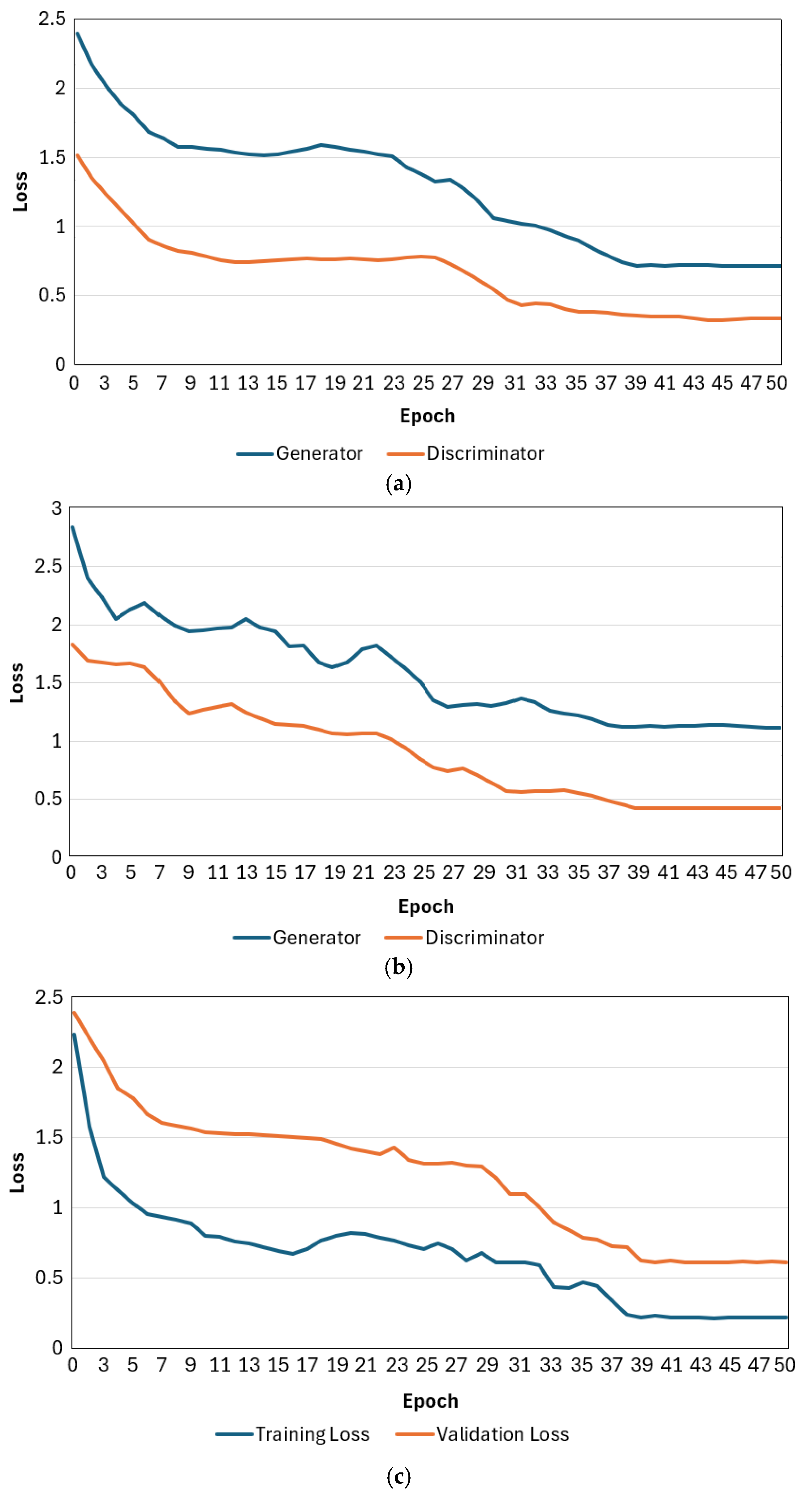
4.1. Training

This subsection describes the software, hardware, hyperparameters used for training, and the training setup used in this study.

Table 2. Software and hardware used in our method.

Hardware		Software
Hardware	Specification	Library	Version
Memory	32 GB RAM	Python [35]	3.5.4
GPU	Nvidia GeForce TITAN X (12 GB)	TensorFlow [36]	1.9.0
CPU	Intel(R) CoreTM i7-6700 CPU@3.40 GHz (8 CPUs)	OpenCV [37]	4.3.0
		Keras API [38]	2.1.6-tf

shows the software and specifications of the computer, and

Table 3. Training setup.

Parameter	Pl-ImC	Pl-ImS
Loss	Categorical cross-entropy (CCE) [39]	Binary cross entropy loss (BCE) [40]
Optimizer	Adaptive moment estimation (Adam) [41]	Adam
# Epochs	100	100
Learning rate	0.001	0.001
Batch size	8	8

summarizes the hyperparameters and training setup of the proposed Pl-ImS and Pl-ImC methods. When choosing the hyperparameters, we optimized them in our experiments by training the models with different hyperparameters. The epoch number was set to 100 for both methods, but we chose a model with 40 epochs because it has the best classification accuracy based on validation data.

Adam optimizer was used in the training, and the loss functions are as follows: The expression for the BCE can be expressed as Equation (6).

$$BCE=-{\displaystyle \frac{1}{N}}{\sum }_{i=1}^N(x\left(i\right)\mathit{log}\left(p\left(i\right)\right)+(1-x\left(i\right)\left)log\right(1-p\left(i\right)\left)\right)$$

(6)

where p(i) and x(i) denote the predicted and true classes of the ith sample, and N denotes the total number of samples, respectively. x is 0 or 1. The expression of CCE loss can be expressed as Equation (7).

$$CCE(o)=-\mathrm{l}\mathrm{o}\mathrm{g}\left({\displaystyle \frac{exp\left(k\right(o\left)\right)}{{\sum }_l^{N}exp\left(k\right(l\left)\right)}}\right)$$

(7)

where exp is an exponential function that is applied to elements in the input vector k and output value ($\mathrm{e}\mathrm{x}\mathrm{p}\left(k\right(o\left)\right)$), followed by a normalization process using the sum of exponentials (${\sum }_l^{N}exp\left(k\right(l\left)\right)$). All experiments were performed using 2-fold cross-validation, where for each fold, half of all data samples are for the train set while the rest is for the test set. We then performed a 2nd fold validation by swapping the testing and training sets. At each fold, the validation subset is obtained from the training data, which is 10% of the training set. We also trained the classification and segmentation networks separately using the dataset. Training the models in a separate way allows the models to focus more on their own tasks (segmentation and classification), which helps to achieve better accuracy.

Moreover, the end-to-end training process that concatenates both segmentation and classification networks requires a longer time for training the parameters. Figure 7 illustrates the loss curves of the training process for the Pl-ImS segmentation method and the Pl-ImC classification method, along with the validation loss curves for each epoch. As the epoch progresses, the loss curves of the training process converge, which means our network is properly trained. Also, the loss curve of the validation process converges as the epoch progresses, which means our network does not overfit.

In addition, in the experimental comparisons with existing methods in this study, we did not fine-tune any pre-trained models to ensure fair comparisons. Instead, their networks, including ours, were trained from scratch using only our self-collected dataset. Moreover, we did not modify the internal architectures or default configurations of the state-of-the-art methods. All models were used as publicly released, with only essential training hyperparameters adjusted as summarized in Table 3. Additionally, the input image sizes were resized to match the required input dimensions of each model to ensure compatibility and optimal performance. For the classification outputs, we set the number of output classes to match our proposed model’s class definitions to enable a fair comparison across all methods.

4.2. Testing

4.2.1. Evaluation Metrics

Two evaluation metrics (Equations (8) and (9)) were used to measure the performance of plant image segmentation. These metrics include calculating the dice score (DS) [42] in Equation (8) and the intersection over union (IoU) [43] in Equation (9). The DS and IoU metrics measure the segmentation accuracy based on the overlapping area of the ground-truth mask and the segmented mask in an image segmentation task.

$$\mathrm{D}\mathrm{S}={\displaystyle \frac{2\times \mathrm{T}\mathrm{P}}{2\times \mathrm{T}\mathrm{P}+\mathrm{F}\mathrm{P}+\mathrm{F}\mathrm{N}}}$$

(8)

$$\mathrm{I}\mathrm{o}\mathrm{U}={\displaystyle \frac{TP}{TP+FP+FN}}$$

(9)

Here, FP, TP, and FN are false positive, true positive, and false negative pixels, respectively, and positive and negative pixels denote pixels that are in the target’s region and pixels that are not in the target’s region, respectively. Thus, FP, TP, and FN refer to pixels that are not in the object’s region but were incorrectly determined to be, pixels that were correctly determined to be, and pixels that were incorrectly determined not to be in the object’s region, respectively. In this study, we also measured the segmentation accuracy based on the similarity between the complexity of the ground-truth segmentation region and the complexity of the segmentation region in the segmented mask based on the fractal dimension (FD) [44], as shown in Equation (10). FD scales the image to compute the complexity of the shape, which indicates whether the structure of the segmented image is distributed or concentrated [44]. In Equation (10), N, j, and FD are the number of boxes, the size of the box, and the fractal dimension, respectively.

$$\mathrm{F}\mathrm{D}={\mathit{lim}}_{ j\to 0}\mathrm{ }{\displaystyle \frac{\mathrm{l}\mathrm{o}\mathrm{g}\left(\mathrm{N}\right(\mathrm{j}\left)\right)}{\mathrm{l}\mathrm{o}\mathrm{g}(1/\mathrm{j})}}$$

(10)

Three metrics (Equations (11)–(13)) were used for measuring the accuracy of classification [43]. The equations are for estimating the F1-score using the positive predictive value (PPV) and the true positive rate (TPR), PPV using true positive (TP) and false positive (FP), and TPR using TP and false negative (FN). The ‘#’ in Equations (11)–(13) represents a count. Here, positive and negative refer to images that are classified as belonging to a certain class and images that are classified as not belonging to a certain class, respectively. TP, FN, and FP refer to cases where images that are classified as belonging to a certain class, which actually belongs to a certain class, cases where images that are classified as not belonging to a certain class, which actually belongs to a certain class, and cases where images that are classified as belonging to a certain class, which does not actually belongs to a certain class.

TPR = #TP/(#TP + #FN)

(11)

PPV = #TP/(#TP + #FP)

(12)

F-score = 2 × PPV × TPR/(PPV + TPR)

(13)

4.2.2. Ablation Study

In this subsection, we present the results of various ablation studies using the self-collected dataset.

Table 4. Segmentation results by the proposed Pl-ImS, in which various numbers of dense blocks were used in the Pl-ImS architecture to determine the optimal architectural configuration (unit: %).

Architectures	DS	IoU
Pl-ImS (with three dense blocks)	88.74	80.18
Pl-ImS (with four dense blocks)	89.19	81.58
Pl-ImS (with five dense blocks)	89.90	81.82
Pl-ImS (with six dense blocks)	89.05	81.58
Pl-ImS (with seven dense blocks)	87.16	79.58

compares the average segmentation results using all images, where various numbers of dense blocks were used in the Pl-ImS architecture to determine the optimal configuration. As shown in Table 4, Pl-ImS with five dense blocks achieved the best performance compared to other architectures. Therefore, this configuration was used for further experiments.

Table 5. Segmentation results by the proposed Pl-ImS (unit: %).

Input Images	DS	IoU
Normal	91.23	82.83
Missing part	89.52	81.46
Little wet leaf with small water droplets	90.06	82.01
Drenched leaf with large water droplets	89.74	81.48
Dust	88.95	81.36
Average	89.90	81.82

compares the segmentation results using all images, including the normal case, images with missing parts, a little wet leaf with small water droplets, a drenched leaf with large water droplets, and dust cases. As shown in Table 5, the segmentation results obtained by Pl-ImS are DS = 89.90% and IoU = 81.82%.

As shown in Table 5, the “Normal” image has the highest accuracy, followed by the “Little wet leaf with small water drop” image. For the “Little wet leaf with small water drop” image, we can see that the size of the water drop on the leaf is small, so it does not affect the accuracy much, while for the “Drenched leaf with large water drop” image, the size of the water drop on the leaf is large, and for the “dust” image, the dust obscures the features and patterns of the leaf, so it affects the accuracy a lot.

As a next ablation study,

Table 6. Classification results by the proposed Pl-ImS + Pl-ImC, in which various numbers of residual blocks were used in the Pl-ImC architecture to determine the optimal architectural configuration (unit: %).

Architectures	Pl-ImS + Pl-ImC
	TPR	PPV	F1-Score
With a residual block	96.36	93.99	95.18
With two residual blocks	96.36	94.52	95.44
With three residual blocks	96.67	95.28	95.97
With four residual blocks	96.29	94.71	95.50
With five residual blocks	96.32	95.26	95.79

compares the average classification results using all images, where various numbers of residual blocks were used in the Pl-ImC architecture to determine the optimal configuration. As shown in Table 6, Pl-ImC with three residual blocks achieved the best performance compared to other architectures. Therefore, this configuration was used for further experiments.

Table 7. Confusion matrix of classification results by the proposed Pl-ImS + Pl-ImC.

	Predicted	Aruncus dioicus	Callicarpa dichotoma	Euonymus fortunei	Lonicera ruprechtiana	Malus floribunda	Populus tremula L.	Vaccinium myrtillus L.	White paeonia	Total # of Data	TPR (%)
Actual
Aruncus dioicus		2289	0	19	14	15	17	1	5	2360	96.99
Callicarpa dichotoma		3	3416	48	23	10	2	9	9	3520	97.05
Euonymus fortunei		33	25	3403	54	16	3	31	35	3600	94.53
Lonicera ruprechtiana		1	12	2	2030	5	20	5	5	2080	97.60
Malus floribunda		11	17	6	12	2100	40	5	9	2200	95.45
Populus tremula L.		1	14	0	5	10	2550	5	15	2600	98.08
Vaccinium myrtillus L.		35	9	15	43	10	15	3100	53	3280	94.51
White paeonia		22	4	12	3	5	16	18	2040	2120	96.23

presents the confusion matrix used to compare the classification performance of each class. As shown, classes with more data, such as Euonymus fortunei (3600 samples, TPR: 94.53%) and Callicarpa dichotoma (3520 samples, TPR: 97.05%), exhibited lower accuracy than those with fewer samples, like Lonicera ruprechtiana (2080 samples, TPR: 97.60%) and Populus tremula L. (2600 samples, TPR: 98.08%). This result confirms that having more data does not necessarily lead to higher classification accuracy.

Moreover, the results of plant classification using ResNet-50 [21], a well-known classification method, are shown in

Table 8. Classification results by ResNet-50 with and without a segmentation (unit: %).

Input Images	ResNet-50			Pl-ImS + ResNet-50
	TPR	PPV	F1-Score	TPR	PPV	F1-Score
Normal	91.51	95.14	93.32	97.74	94.49	96.11
Missing part	88.59	89.25	88.92	93.02	92.78	92.90
Little wet leaf with small water drop	86.59	86.36	86.47	95.16	92.14	93.65
Drenched leaf with large water drop	90.22	94.46	92.34	94.90	93.40	94.15
Dust	90.08	87.07	88.57	93.96	91.82	92.89
Average	89.39	90.45	89.92	94.95	92.92	93.94

. The accuracy of the combined method of the Pl-ImS and ResNet-50 proposed in this paper is also compared. In Table 8, ResNet has the lowest accuracy for “Little wet leaf with small water drop” images, but Pl-ImS + ResNet-50 has the lowest accuracy for “Dust” images, which is analyzed to be due to the lowest segmentation accuracy for “Dust” images in Table 5.

Also, as shown in Table 8, the accuracy of Pl-ImS + ResNet-50 is significantly higher than the classification accuracy of ResNet-50 without Pl-ImS. As a result, it can be seen that the classification accuracy is higher when the segmentation model (Pl-ImS) is applied before the classification model (ResNet-50). Then, the accuracy of Pl-ImC and Pl-ImS + Pl-ImC proposed in this paper is compared as shown in

Table 9. Classification results by the proposed Pl-ImC with and without Pl-ImS (unit: %).

Input Images	Pl-ImC			Pl-ImS + Pl-ImC
	TPR	PPV	F1-Score	TPR	PPV	F1-Score
Normal	94.56	97.51	96.03	98.23	97.35	97.79
Missing part	90.14	90.90	90.52	95.44	94.82	95.13
Little wet leaf with small water drop	88.70	89.77	89.23	95.95	93.66	94.80
Drenched leaf with large water drop	92.37	96.17	94.27	97.18	96.15	96.66
Dust	93.76	88.27	91.01	96.57	94.42	95.49
Average	91.90	92.52	92.21	96.67	95.28	95.97

. As shown in Table 8 and Table 9, the accuracy of the proposed Pl-ImC is higher than the classification results using ResNet-50, and the accuracy using Pl-ImS is significantly the highest.

4.2.3. Comparisons with Plant Image-Based SOTA Segmentation Methods

Next, we compared our method with previously introduced plant image segmentation-based SOTA methods. As a comparison method, segmentation methods based on structures such as DeepLabV3+ [22], Modified U-Net [23], YOLOv8-Seg [17], Mask R-CNN [24], and CNN-SS [26] were used.

Table 10. Comparisons of segmentation accuracies by the proposed and SOTA methods (unit: %).

Input Images	Model/Method	DS	IoU
Normal	DeepLabV3+ [22]	84.93	81.35
	YOLOv8-Seg [17]	83.74	79.41
	Mask R-CNN [24]	83.84	79.56
	Modified U-Net [23]	83.48	80.48
	CNN-SS [26]	84.52	81.65
	Pl-ImS (proposed)	91.23	82.83
Missing part	DeepLabV3+ [22]	83.62	80.13
	YOLOv8-Seg [17]	82.29	78.12
	Mask R-CNN [24]	82.34	78.37
	Modified U-Net [23]	82.52	79.78
	CNN-SS [26]	83.41	80.13
	Pl-ImS (proposed)	89.52	81.46
Little wet leaf with small water drop	DeepLabV3+ [22]	84.43	80.91
	YOLOv8-Seg [17]	82.89	79.14
	Mask R-CNN [24]	83.09	79.72
	Modified U-Net [23]	82.85	79.92
	CNN-SS [26]	83.88	81.08
	Pl-ImS (proposed)	90.06	82.01
Drenched leaf with large water drop	DeepLabV3+ [22]	84.33	80.40
	YOLOv8-Seg [17]	82.39	78.88
	Mask R-CNN [24]	82.93	78.86
	Modified U-Net [23]	82.69	79.79
	CNN-SS [26]	83.60	80.28
	Pl- ImS (proposed)	89.74	81.48
Dust	DeepLabV3+ [22]	83.06	80.11
	YOLOv8-Seg [17]	81.70	78.37
	Mask R-CNN [24]	82.17	78.18
	Modified U-Net [23]	81.60	79.49
	CNN-SS [26]	81.80	80.11
	Pl-ImS (proposed)	88.95	81.36
Average	DeepLabV3+ [22]	84.07	80.58
	YOLOv8-Seg [17]	82.60	78.78
	Mask R-CNN [24]	82.87	78.93
	Modified U-Net [23]	82.62	79.89
	CNN-SS [26]	83.44	80.65
	Pl-ImS (proposed)	89.90	81.82

compares the segmentation performance, and

Table 11. Comparisons of classification accuracies by the proposed and SOTA segmentation methods, followed by ResNet-50 (unit: %).

Input Images	Model/Method	TPR	PPV	F1-Score
Normal	DeepLabV3+ [22] + ResNet-50	87.45	90.64	89.04
	YOLOv8-Seg [17] + ResNet-50	88.34	88.41	88.37
	Mask R-CNN [24] + ResNet-50	95.12	89.43	92.27
	Modified U-Net [23] + ResNet-50	92.56	89.18	90.87
	CNN-SS [26] + ResNet-50	89.78	94.71	92.24
	Pl-ImS + ResNet-50	97.74	94.49	96.11
Missing part	DeepLabV3+ [22] + ResNet-50	86.18	93.05	89.61
	YOLOv8-Seg [17] + ResNet-50	89.37	89.60	89.48
	Mask R-CNN [24] + ResNet-50	91.06	90.17	90.61
	Modified U-Net [23] + ResNet-50	90.03	87.02	88.52
	CNN-SS [26] + ResNet-50	91.87	87.23	89.55
	Pl-ImS + ResNet-50	93.02	92.78	92.90
Little wet leaf with small water drop	DeepLabV3+ [22] + ResNet-50	85.57	88.01	86.79
	YOLOv8-Seg [17] + ResNet-50	86.80	86.98	86.89
	Mask R-CNN [24] + ResNet-50	93.58	87.06	90.32
	Modified U-Net [23] + ResNet-50	90.56	87.86	89.21
	CNN-SS [26] + ResNet-50	87.74	92.08	89.91
	Pl-ImS + ResNet-50	95.16	92.14	93.65
Drenched leaf with large water drop	DeepLabV3+ [22] + ResNet-50	91.62	88.40	90.01
	YOLOv8-Seg [17] + ResNet-50	90.96	94.86	92.91
	Mask R-CNN [24] + ResNet-50	85.68	88.72	87.20
	Modified U-Net [23] + ResNet-50	92.64	94.88	93.76
	CNN-SS [26] + ResNet-50	88.20	89.55	88.87
	Pl-ImS + ResNet-50	94.90	93.40	94.15
Dust	DeepLabV3+ [22] + ResNet-50	89.11	94.38	91.74
	YOLOv8-Seg [17] + ResNet-50	92.08	88.69	90.38
	Mask R-CNN [24] + ResNet-50	91.26	93.01	92.13
	Modified U-Net [23] + ResNet-50	88.29	88.40	88.34
	CNN-SS [26] + ResNet-50	94.96	89.37	92.16
	Pl-ImS + ResNet-50	93.96	91.82	92.89
Average	DeepLabV3+ [22] + ResNet-50	87.98	90.89	89.44
	YOLOv8-Seg [17] + ResNet-50	89.51	89.70	89.60
	Mask R-CNN [24] + ResNet-50	91.34	89.67	90.50
	Modified U-Net [23] + ResNet-50	90.81	89.46	90.14
	CNN-SS [26] + ResNet-50	90.51	90.58	90.54
	Pl-ImS + ResNet-50	94.95	92.92	93.94

shows how each segmentation method affects the classification performance. As shown in Table 10, the segmentation accuracy of Pl-ImS is higher than that of the previously introduced plant image segmentation-based SOTA methods. Also, as in Table 11, the classification accuracy of the proposed Pl-ImS is greater than the classification results using the previously introduced plant image segmentation-based SOTA methods.

Therefore, it can be seen that the proposed Pl-ImS method achieves the highest accuracy in the segmentation (Table 10) and classification (Table 11) tasks. However, for other SOTA segmentation methods, the accuracy rankings are different in Table 10 and Table 11. Also, the proposed method has the highest accuracy when using “Normal” images, but the accuracy rankings are different for other SOTA segmentation methods. This shows that each SOTA segmentation method has a different network structure, does not produce similar results for each image dataset, and has different features.

4.2.4. Comparisons with Plant Image-Based SOTA Classification Methods

Next, we compared the proposed classification method with existing plant image-based SOTA classification methods. ANN-based [45], EfficientNet B5 [46], SVM-based [47], CNN-GLS [48], and CNN-SS [26] were used as comparison methods. The classification performance is compared in

Table 12. Comparisons of classification accuracies by the proposed and SOTA methods (unit: %).

Input Images	Model/Method	TPR	PPV	F1-Score
Normal	ANN-based [45]	93.01	93.84	93.43
	EfficientNet B5 [46]	92.25	92.64	92.45
	SVM-based [47]	93.15	95.78	94.47
	CNN-GLS [48]	92.45	96.45	94.45
	CNN-SS [26]	93.49	95.04	94.27
	Pl-ImC	94.56	97.51	96.04
	Pl-ImS + Pl-ImC (proposed)	98.23	97.35	97.79
Missing part	ANN-based [45]	89.57	90.20	89.88
	EfficientNet B5 [46]	90.04	90.40	90.22
	SVM-based [47]	89.13	89.71	89.42
	CNN-GLS [48]	89.00	90.84	89.92
	CNN-SS [26]	89.90	90.32	90.11
	Pl-ImC	90.14	90.90	90.52
	Pl-ImS + Pl-ImC (proposed)	95.44	94.82	95.13
Little wet leaf with small water drop	ANN-based [45]	87.31	87.97	87.64
	EfficientNet B5 [46]	87.93	87.46	87.70
	SVM-based [47]	87.41	87.00	87.20
	CNN-GLS [48]	87.26	87.27	87.26
	CNN-SS [26]	87.16	87.35	87.25
	Pl-ImC	88.70	89.77	89.24
	Pl-ImS + Pl-ImC (proposed)	95.95	93.66	94.80
Drenched leaf with large water drop	ANN-based [45]	90.56	95.20	92.88
	EfficientNet B5 [46]	91.48	95.09	93.28
	SVM-based [47]	90.77	95.30	93.04
	CNN-GLS [48]	90.84	95.88	93.36
	CNN-SS [26]	91.33	96.08	93.71
	Pl-ImC	92.37	96.17	94.27
	Pl-ImS + Pl-ImC (proposed)	97.18	96.15	96.66
Dust	ANN-based [45]	91.37	88.34	89.85
	EfficientNet B5 [46]	91.07	88.54	89.81
	SVM-based [47]	91.09	87.34	89.21
	CNN-GLS [48]	91.46	88.30	89.88
	CNN-SS [26]	91.97	87.74	89.85
	Pl-ImC	93.76	88.27	91.02
	Pl-ImS + Pl-ImC (proposed)	96.57	94.42	95.49
Average	ANN-based [45]	90.36	91.11	90.74
	EfficientNet B5 [46]	90.55	90.83	90.69
	SVM-based [47]	90.31	91.03	90.67
	CNN-GLS [48]	90.20	91.75	90.97
	CNN-SS [26]	90.77	91.31	91.04
	Pl-ImC	91.91	92.52	92.22
	Pl-ImS + Pl-ImC (proposed)	96.67	95.28	95.97

, and it can be seen that the proposed Pl-ImS + Pl-ImC results are higher than the results of existing plant image-based SOTA classification methods.

The proposed method has the highest accuracy when using “Normal” images, but for other SOTA classification methods, the accuracy rankings are different: most of them have high accuracy when using “Normal” images, and most of them have low accuracy when using “Little wet leaf with small water drop” images. This shows that the network structure of each SOTA classification method is different and has different functions.

4.2.5. Comparisons of Algorithm Complexity

In this subsection, we compare the algorithmic complexity between the proposed method and existing SOTA methods in the desktop computer environment described in Table 2. The deep learning methods described in Section 4.2.4 were used for comparison.

Table 13. Comparisons of processing times, GFLOPs, # parameters, and model sizes of proposed and SOTA methods (# means ‘number of’).

Model	Processing Time (Unit: ms)	GFLOPs	# Parameters (unit: Mega)	Model Size (Unit: MB)
ANN-based [45]	122.7	108.4	5.4	24.7
EfficientNet B5 [46]	135.8	115	30	56.4
CNN-GLS [48]	118.2	92.9	3.1	30.4
CNN-SS [26]	110.4	91.2	2.5	23.2
Pl-ImS + Pl-ImC (proposed)	151.4	131.2	123.0	62.0

shows the processing time per image, giga floating-point operations (GFLOPs), number of parameters, and model size. As shown in Table 13, our method does not have the lowest algorithmic complexity, which is due to the fact that our method additionally utilizes a segmentation model, which results in higher algorithmic complexity than other methods. However, in terms of classification accuracy, which is the main goal of this study, our method outperforms all existing SOTA methods, as shown in Table 12. In addition,

Table 14. Comparisons of processing times for real-time performance on relevant hardware platforms.

#	Device/Chipset	Architecture	Year	Estimated Time (ms)
1	GTX Titan X (ours)	Maxwell	2015	151.4
2	GTX 1060 6GB	Pascal	2016	204.8
3	GTX 1070	Pascal	2016	156.2
4	GTX 1080	Pascal	2016	113.9
5	RTX 2080 Ti	Turing	2018	38.1
6	GTX 1650	Turing	2019	302.8
7	RTX 2060	Turing	2019	78.5
8	Snapdragon 865 (Galaxy S20)	Android (Adreno 650)	2020	25,233.3
9	RTX 3090	Ampere	2020	28.7
10	Jetson Xavier NX (FP16)	Volta	2020	3028.0
11	Snapdragon 888 (Galaxy S21)	Android (Adreno 660)	2021	18,925.0
12	RTX 3060	Ampere	2021	79.7
13	Apple A15 Bionic (iPhone 13)	iOS (Neural Engine)	2021	9462.5
14	RTX 4090	Ada Lovelace	2022	12.3
15	Apple M2 (iPad Pro/MacBook)	macOS (Neural Eng.)	2022	1009.3
16	Snapdragon 8 Gen 2 (Galaxy S23)	Android (Adreno 740)	2022	12,616.7
17	Apple A16 Bionic (iPhone 14)	iOS (Neural Engine)	2022	8411.1
18	Jetson Orin Nano (INT8)	Ampere	2023	1514.0
19	RTX 4060	Ada Lovelace	2023	67.9

provides a comparison of processing times as a benchmark for real-time performance across 19 relevant hardware platforms.

5. Discussion

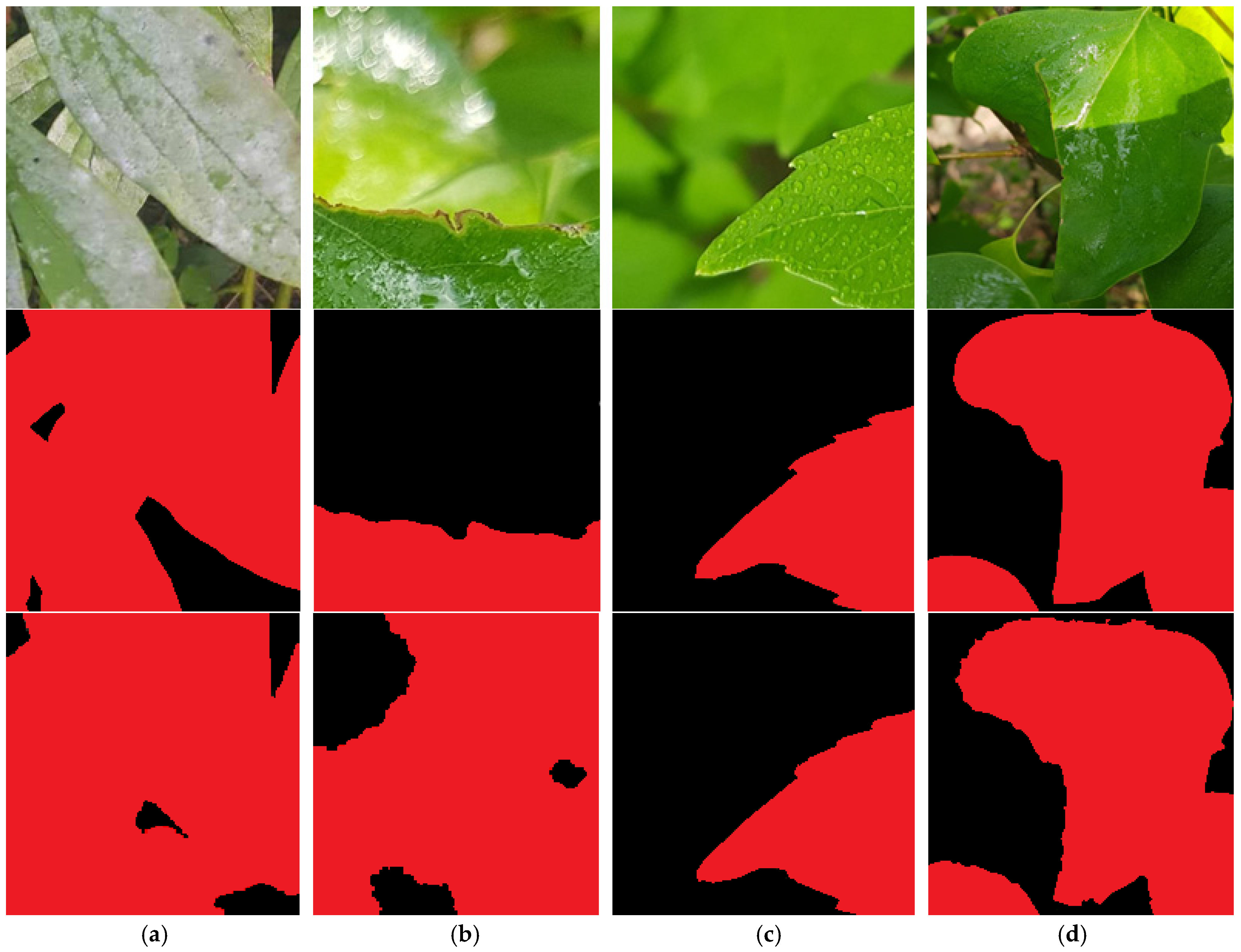
5.1. Error and Correct Segmentation Cases

Figure 8 shows the segmentation error and correct segmentation cases generated by the proposed Pl-ImS. In Figure 8a, the input image was covered with dust, which caused the segmentation error. In Figure 8b, the input image was missing some parts of the plant, and the remaining plant parts were blurred, which caused the segmentation error. However, as shown in Figure 8c,d, the proposed Pl-ImS segmented the plant image well even when some parts were removed.

5.2. Error and Correct Classification Cases

Figure 9 shows the classification errors and correct classification cases made by the proposed Pl-ImC. In Figure 9a, the input image was covered with dust, which caused the recognition error. In Figure 9b, the input image was missing some parts of the plant, and the rest of the plant was blurred, which caused the error. However, as shown in Figure 9c,d, the plant image was recognized well even when some parts were missing. We also analyzed the gradient-weighted class activation mapping (Grad-CAM) [49] images to verify that the proposed model extracts important features (red and yellow colors in Figure 9) for accurate classification and to interpret the model’s decision.

This Grad-CAM image is extracted from the last convolution layer of the proposed Pl-ImC. As shown in the Grad-CAM images in Figure 9, we can see that a plant in the image is correctly classified when focusing on the non-blurry image parts of the plant leaves (Figure 9c,d), whereas the image with dust (Figure 9a) and blurry parts (Figure 9b) are incorrectly classified when they are focused.

As shown in Figure 8 and Figure 9, blur and dust interfere with the extraction of clear texture and edge features, which are essential for both accurate segmentation of plant leaf boundaries and classification of disease patterns. The segmentation model, in particular, relies on contrast and structure to distinguish high-quality plant regions, and the presence of dust or motion blur can obscure these cues, leading to segmentation leakage or omission. This mis-segmentation then propagates to the classification stage, resulting in increased misclassifications due to irrelevant or misleading features being passed to the classifier, and this provides concrete evidence of how visual degradation affects each stage of the model pipeline.

5.3. FD Estimation for Plant Image Segmentation

In this subsection, we measure the segmentation accuracy based on the similarity between the complexity of the ground-truth segmentation region and the complexity of the segmentation region in the segmentation mask based on the FD, as shown in Equation (10). Figure 10 shows the input image, ground-truth segmentation mask image, and segmented images by various methods. Figure S6 (Supplementary Materials) illustrates the FD analysis performed using the segmented images shown in Figure 10.

Table S9 (Supplementary Materials) compares the segmentation performance of each method using the correlation coefficient (C), the coefficient of determination (R2), and the FD values. C value in Table S9 measures the linear relationship between two sets of values. In segmentation, it is used when comparing segmentation probability maps, where a C value closer to 1 means that the predicted pixel intensities closely match the ground-truth trends. The R² value in Table S9 indicates how much of the variance in the ground-truth is explained by the prediction. In segmentation, it evaluates how well predicted segmentation probability maps track the ground-truth, where an R² value closer to 1 indicates that the prediction explains most of the variation in the ground-truth.

FD quantifies the complexity or irregularity of a shape, especially its boundary. In segmentation, it is often used to characterize the shape of the segmented object, how rough, intricate, or detailed its edges are. A higher FD value means a more complex, irregular shape. In segmentation, we compute the FD of both the predicted and ground-truth segment boundaries. If their FD values are close, it suggests that the predicted segmentation captures the same level of structural detail as the ground-truth.

Moreover, DS and IoU measure the area or region of overlap; in short, they compare the segmentation result image and the ground-truth image by overlapping them to assess shape similarity, whereas FD compares only the edges (boundaries).

The images in Figure 10a and Figure 10b–h are the input color image and binary image, respectively, where white regions represent objects and black regions represent background. As shown in Figure 10, the binary image (c) segmented by the proposed method is the most similar to the ground-truth segmentation mask (b).

The binary images shown in Figure 10 are used for subsequent FD analysis. The data for calculating FD is obtained by covering the binary image with boxes of different sizes and counting the number of boxes that intersect the plant. The FD values in Figure S6 indicate how irregular and complex the shape of the segmented image is. As shown in Figure S6, lower FD values indicate less complex shapes, while higher values indicate more complex shapes.

In Table S9, “Box#” refers to the total number of boxes, including the different-sized boxes shown on the left side of Figure S6. Also, “S#” indicates the number of boxes of different sizes used in the FD value calculation. Here we can see that due to the complex shape of the image, we did not analyze it using the same-sized boxes. The largest and smallest box sizes are 128 × 128 and 2 × 2, respectively. A higher number of boxes means that more boxes are required to analyze the image, which means the shape is more complex. In addition, the image segmented by CNN-SS [26] (Figure 10f) had the lowest FD value due to fewer convex defects compared to the other images. Moreover, the higher FD value (YOLOv8-Seg in Figure 10e) indicates that the image used more boxes to analyze it compared to the other images, indicating that an image segmented by YOLOv8-Seg [24] was of higher complexity compared to the other images.

In addition, the FD, C, R2 values, and Box#, S#, s# obtained by Pl-ImS on this image are most similar to the ground-truth mask image compared to other images, as shown in Table S9. This confirms that the binary image segmented by the proposed Pl-ImS is more similar to the ground-truth mask image compared to other images, which means that the proposed Pl-ImS has better segmentation performance compared to other methods. Also, in Table S9, “s#” indicates the number of smallest boxes (2 × 2 size) used in the image analysis. The image segmented by Modified U-Net [23] used the most 58,617 smallest boxes in Table S9, which means that it has more undesirable small convex defects than the other images. In addition, the image segmented with our proposed method has the fewest smallest boxes in Table S9, 44,543, which means that it has fewer small convex defects than the other four images.

5.4. Statistical Analysis

In addition, a t-test (Student’s t-test [50]) and Cohen’s d-value [51] have been calculated (Figure S7 (Supplementary Materials)) for statistical validation using the dataset. To conduct the statistical validation, the F1 scores of our method and the second-best method are among the methods shown in Table S9. Cohen’s d-values, which are around 0.2, 0.5, and 0.8, represent effective sizes; the greater value indicates higher effectiveness. Cohen’s d-value and the p-value between our method and the second-best (CNN-SS [26]) method were calculated by using our newly collected plant image dataset as explained in Section 3.4. Cohen’s d-value and the p-value of the results obtained from the self-collected dataset were 0.046 and 5.552, respectively. The results above indicate that the proposed method achieves statistically greater accuracy compared to the second-best one in the confidence level of 95% with a large effect size.

6. Conclusions

In this study, we investigated for the first time how to recognize plants by ignoring blurred areas in the image and focusing only on clearly visible leaf areas. In addition, we acquired and studied a plant image dataset with complex backgrounds in a real field environment, where various factors play a role, including the surface of the plant in the input image being covered with moisture, water droplets, dust, etc., and some areas of the leaf being lost. To solve the problem of misclassifying plant images in these studies, we proposed a new method that combines Pl-ImS, a plant segmentation model, and Pl-ImC, a plant classification network.

Through various experiments using self-collected image datasets, we have shown that the proposed method achieves high classification accuracy, outperforming some existing methods. The t-test and Cohen’s d-value demonstrate that our method is statistically better than the existing methods. Moreover, we have demonstrated that our method correctly focuses on the regions with important information in the input plant images and performs classification based on Grad-CAM. Additionally, our method improved the plant classification and segmentation performance, as shown in Table 8 and Table 9. When the segmentation model was added to the proposed classification model, it showed greater accuracy compared to the previously introduced plant image-based classification model. This shows that the segmentation model is an effective addition to the classification task. Additionally, we also conducted an analysis of the segmentation results by using FD estimation. The FD values calculated by using the images generated by our method and the ground-truth mask images were most similar, as shown in the segmentation results.

However, as shown in the discussion section, our method performed classification and segmentation effectively when the input image contained only minimal plant information. Additionally, the experimental results show that the classification performance is very poor when there is a lot of dust. However, we have developed a model that effectively recognizes images of plants with some parts removed. In addition, even in images of plant leaves with some parts missing, we can see that the remaining parts of the plant are well-focused and correctly classified.

In future work, we will add more images of various plants, including environmental cases, to the self-collected dataset to reduce the errors and develop the proposed classification and segmentation networks to reflect the features of the SOTA methods. In addition, we will study how the complexity of the proposed models and algorithms can be reduced by using methods such as knowledge distillation and parameter quantization.

References

1. Batchuluun, G.; Nam, S.H.; Park, K.R. Deep learning-based plant classification and crop disease classification by thermal camera. J. King Saud Univ.-Comput. Inf. Sci. 2022, 34, 1319–1578. [Google Scholar] [CrossRef]
2. Anasta, N.; Setyawan, F.X.A.; Fitriawan, H. Disease detection in banana trees using an image processing-based thermal camera. IOP Conf. Ser. Earth Environ. Sci. 2021, 739, 012088. [Google Scholar] [CrossRef]
3. Raza, S.E.; Prince, G.; Clarkson, J.P.; Rajpoot, N.M. Automatic detection of diseased tomato plants using thermal and stereo visible light images. PLoS ONE 2015, 10, e0123262. [Google Scholar] [CrossRef] [PubMed]
4. Zhu, W.; Chen, H.; Ciechanowska, I.; Spaner, D. Application of infrared thermal imaging for the rapid diagnosis of crop disease. IFAC-Pap. 2018, 51, 424–430. [Google Scholar] [CrossRef]
5. Shahi, T.B.; Sitaula, C.; Neupane, A.; Guo, W. Fruit classification using attention-based MobileNetV2 for industrial applications. PLoS ONE 2022, 17, e0264586. [Google Scholar] [CrossRef] [PubMed]
6. Kader, A.; Sharif, S.; Bhowmick, P.; Mim, F.H.; Srizon, A.Y. Effective workflow for high-performance recognition of fruits using machine learning approaches. Int. Res. J. Eng. Technol. 2020, 7, 1516–1521. [Google Scholar]
7. Biswas, B.; Ghosh, S.K.; Ghosh, A. A robust multi-label fruit classification based on deep convolution neural network. In Computational Intelligence in Pattern Recognition; Advances in Intelligent Systems and Computing; Das, A., Nayak, J., Naik, B., Pati, S., Pelusi, D., Eds.; Springer: Singapore, 2020; Volume 999. [Google Scholar] [CrossRef]
8. Hossain, M.S.; Al-Hammadi, M.; Muhammad, G. Automatic fruit classification using deep learning for industrial applications. IEEE Trans. Ind. Inform. 2019, 15, 1027–1034. [Google Scholar] [CrossRef]
9. Abawatew, G.Y.; Belay, S.; Gedamu, K.; Assefa, M.; Ayalew, M.; Oluwasanmi, A.; Qin, Z. Attention augmented residual network for tomato disease detection and classification. Turk. J. Electr. Eng. Comput. Sci. 2021, 29, 2869–2885. [Google Scholar] [CrossRef]
10. Ashwinkumar, S.; Rajagopal, S.; Manimaran, V.; Jegajothi, B. Automated plant leaf disease detection and classification using optimal MobileNet based convolutional neural networks. Mater. Today 2022, 51, 480–487. [Google Scholar] [CrossRef]
11. Chakraborty, A.; Kumer, D.; Deeba, K. Plant leaf disease recognition using Fastai image classification. In Proceedings of the 5th International Conference on Computing Methodologies and Communication, Erode, India, 8–10 April 2021; pp. 1624–1630. [Google Scholar] [CrossRef]
12. Wang, D.; Wang, J.; Li, W.; Guan, P. T-CNN: Trilinear convolutional neural networks model for visual detection of plant diseases. Comput. Electron. Agric. 2021, 190, 106468. [Google Scholar] [CrossRef]
13. Yun, C.; Kim, Y.W.; Lee, S.J.; Im, S.J.; Park, K.R. WRA-Net: Wide receptive field attention network for motion deblurring in crop and weed image. Plant Phenomics 2023, 5, 0031. [Google Scholar] [CrossRef] [PubMed]
14. Wang, J.; Wu, B.; Kohnen, M.V.; Lin, D.; Yang, C.; Wang, X.; Qiang, A.; Liu, W.; Kang, J.; Li, H.; et al. Classification of rice yield using UAV-based hyperspectral imagery and lodging feature. Plant Phenomics 2021, 2021, 9765952. [Google Scholar] [CrossRef] [PubMed]
15. PlantVillage Dataset. Available online: https://www.kaggle.com/datasets/emmarex/plantdisease (accessed on 8 January 2025).
16. Horea, M.; Mihai, O. Fruit recognition from images using deep learning. Acta Univ. Sapientiae Inform. 2018, 10, 26–42. [Google Scholar]
17. Wang, P.; Deng, H.; Guo, J.; Ji, S.; Meng, D.; Bao, J.; Zuo, P. Leaf segmentation using modified YOLOv8-seg models. Life 2024, 14, 780. [Google Scholar] [CrossRef] [PubMed]
18. Singh, D.; Jain, N.; Jain, P.; Kayal, P.; Kumawat, S.; Batra, N. PlantDoc: A dataset for visual plant disease detection. In Proceedings of the ACM India Joint International Conference on Data Science and Management of Data (CoDS-COMAD), Hyderabad, India, 5–7 January 2020; pp. 249–253. [Google Scholar] [CrossRef]
19. The Self-Collected Dataset and the Source Code. Available online: https://github.com/ganav/Pl-ImS-Pl-ImC (accessed on 18 March 2025).
20. Goodfellow, I.J.; Pouget-Abadie, J.; Mirza, M.; Xu, B.; Warde-Farley, D.; Ozair, S.; Courville, A.; Bengio, Y. Generative adversarial networks. arXiv 2014, arXiv:1406.2661v1. [Google Scholar] [CrossRef]
21. He, K.; Zhang, X.; Ren, S.; Sun, J. Deep residual learning for image recognition. In Proceedings of the 2016 IEEE Conference on Computer Vision and Pattern Recognition (CVPR), Las Vegas, NV, USA; 27–30 June 2016; pp. 770–778. [CrossRef]
22. Yang, T.; Zhou, S.; Xu, A.; Ye, J.; Yin, J. An approach for plant leaf image segmentation based on YOLOV8 and the improved DEEPLABV3+. Plants 2023, 12, 3438. [Google Scholar] [CrossRef] [PubMed]
23. Shoaib, M.; Hussain, T.; Shah, B.; Ullah, I.; Shah, S.M.; Ali, F.; Park, S.H. Deep learning-based segmentation and classification of leaf images for detection of tomato plant disease. Front. Plant Sci. 2022, 13, 1031748. [Google Scholar] [CrossRef] [PubMed]
24. Ward, D.; Moghadam, P.; Hudson, N. Deep leaf segmentation using synthetic data. arXiv 2018, arXiv:1807.10931. [Google Scholar]
25. He, K.; Gkioxari, G.; Dollar, P.; Girshick, R. Mask R-CNN. In Proceedings of the IEEE International Conference on Computer Vision, Venice, Italy, 22–29 October 2017; pp. 2980–2988. [Google Scholar]
26. Milioto, A.; Lottes, P.; Stachniss, C. Real-time semantic segmentation of crop and weed for precision agriculture robots leveraging background knowledge in CNNs. In Proceedings of the IEEE International Conference on Robotics and Automation (ICRA), Brisbane, Australia, 21–25 May 2018; pp. 2229–2235. [Google Scholar]
27. Hamid, N.N.A.A.; Razali, R.A.; Ibrahim, Z. Comparing bags of features, conventional convolutional neural network and AlexNet for fruit recognition. Indones. J. Elect. Eng. Comput. Sci. 2019, 14, 333–339. [Google Scholar] [CrossRef]
28. Katarzyna, R.; Paweł, M.A. Vision-based method utilizing deep convolutional neural networks for fruit variety classification in uncertainty conditions of retail sales. Appl. Sci. 2019, 9, 3971. [Google Scholar] [CrossRef]
29. Siddiqi, R. Comparative performance of various deep learning based models in fruit image classification. In Proceedings of the 11th International Conference on Advances in Information Technology, Bangkok, Thailand, 1–3 July 2020; pp. 1–9. [Google Scholar] [CrossRef]
30. Huang, G.; Liu, Z.; Van Der Maaten, L.; Weinberger, K.Q. Densely connected convolutional networks. arXiv 2016, arXiv:1608.06993. [Google Scholar]
31. Chompookham, T.; Surinta, O. Ensemble methods with deep convolutional neural networks for plant leaf recognition. ICIC Express Lett. 2021, 15, 553–565. [Google Scholar]
32. Batchuluun, G.; Nam, S.H.; Park, K.R. Deep learning-based plant classification using nonaligned thermal and visible light images. Mathematics 2022, 10, 4053. [Google Scholar] [CrossRef]
33. Analysis of Variance. Available online: https://en.wikipedia.org/wiki/Analysis_of_variance (accessed on 8 February 2024).
34. Batchuluun, G.; Nam, S.H.; Park, C.; Park, K.R. Super-resolution reconstruction based plant image classification using thermal and visible-light images. Mathematics 2023, 11, 76. [Google Scholar] [CrossRef]
35. Python. Available online: https://www.python.org/ (accessed on 8 January 2025).
36. TensorFlow. Available online: https://www.tensorflow.org/ (accessed on 8 January 2025).
37. OpenCV. Available online: http://opencv.org/ (accessed on 8 January 2025).
38. Chollet, F. Keras, California, U.S. Available online: https://keras.io/ (accessed on 8 January 2025).
39. Zhang, Z.; Sabuncu, M.R. Generalized cross entropy loss for training deep neural networks with noisy labels. arXiv 2018, arXiv:1805.07836. [Google Scholar]
40. Wali, R. Xtreme Margin: A tunable loss function for binary classification problems. arXiv 2022, arXiv:2211.00176. [Google Scholar]
41. Kingma, D.P.; Ba, J.B. ADAM: A method for stochastic optimization. In Proceedings of the 3rd International Conference on Learning Representations, San Diego, CA, USA, 7–9 May 2015; pp. 1–15. [Google Scholar]
42. Bertels, J.; Eelbode, T.; Berman, M.; Vandermeulen, D.; Maes, F.; Bisschops, R.; Blaschko, M.B. Optimizing the dice score and jaccard index for medical image segmentation: Theory & practice. In Proceedings of the 22nd International Conference on Medical Image Computing and Computer-Assisted Intervention, Shenzhen, China, 13–17 October 2019; pp. 92–100. [Google Scholar]
43. Terven, J.; Cordova-Esparza, D.M.; Romero-González, J.A.; Ramírez-Pedraza, A.; Chávez-Urbiola, E.A. A comprehensive survey of loss functions and metrics in deep learning. Artif. Intell. Rev. 2025, 58, 195. [Google Scholar] [CrossRef]
44. Brouty, X.; Garcin, M. Fractal properties, information theory, and market efficiency. Chaos Solitons Fractals 2024, 180, 114543. [Google Scholar] [CrossRef]
45. Huixian, J. The analysis of plants image recognition based on deep learning and artificial neural network. IEEE Access 2020, 8, 68828–68841. [Google Scholar] [CrossRef]
46. Arun, Y.; Viknesh, G.S. Leaf classification for plant recognition using EfficientNet architecture. In Proceedings of the IEEE Fourth International Conference on Advances in Electronics, Computers and Communications, Bengaluru, India, 10–11 January 2022; pp. 1–5. [Google Scholar] [CrossRef]
47. Keerthika, P.; Devi, R.M.; Prasad, S.J.S.; Venkatesan, R.; Gunasekaran, H.; Sudha, K. Plant classification based on grey wolf optimizer based support vector machine (GOS) algorithm. In Proceedings of the 7th International Conference on Computing Methodologies and Communication, Erode, India, 23–25 February 2023; pp. 902–906. [Google Scholar] [CrossRef]
48. Sun, Y.; Tian, B.; Ni, C.; Wang, X.; Fei, C.; Chen, Q. Image classification of small sample grape leaves based on deep learning. In Proceedings of the IEEE 7th Information Technology and Mechatronics Engineering Conference, Chongqing, China, 15–17 September 2023; pp. 1874–1878. [Google Scholar] [CrossRef]
49. Selvaraju, R.R.; Cogswell, M.; Das, A.; Vedantam, R.; Parikh, D.; Batra, D. Grad-CAM: Visual explanations from deep networks via gradient-based localization. arXiv 2016, arXiv:1610.02391. [Google Scholar]
50. Curtis, D. Welch’s t test is more sensitive to real world violations of distributional assumptions than student’s t test but logistic regression is more robust than either. Stat. Pap. 2024, 65, 3981–3989. [Google Scholar] [CrossRef]
51. Groß, J.; Möller, A. Some additional remarks on statistical properties of Cohen’s d in the presence of covariates. Stat. Pap. 2024, 65, 3971–3979. [Google Scholar] [CrossRef]
Figure 1. Example plant images from the self-collected dataset [19]. (ad) Images containing full leaves; (eh) images with leaf fragments.
Horticulturae 11 00843 g001
Figure 2. Example plant images from the self-collected dataset [19]. (a,b) Plants with little wet leaves with small water droplets; (c,d) plants with drenched leaves and large water droplets; (eh) plants covered in environmental dust.
Horticulturae 11 00843 g002
Figure 3. Example plant images (1st and 2nd rows) with insect-induced damage from the self-collected dataset [19].
Horticulturae 11 00843 g003
Figure 4. Flowchart of the proposed method.
Horticulturae 11 00843 g004
Figure 5. Architecture of the proposed segmentation method. (a) Training phase; (b) testing phase.
Horticulturae 11 00843 g005
Figure 6. Architecture of the proposed Pl-ImC.
Horticulturae 11 00843 g006
Figure 7. Training and validation loss curves of the proposed Pl-ImS and Pl-ImC. (a) Training loss curves of Pl-ImS; (b) validation loss curves of Pl-ImS; (c) training and validation loss curves of Pl-ImC.
Horticulturae 11 00843 g007
Figure 8. Examples of incorrectly or correctly segmented images. From top to bottom, input images, ground-truth masks, and segmentation results: (a,b) incorrectly segmented images; (c,d) correctly segmented images.
Horticulturae 11 00843 g008
Figure 9. Examples of incorrectly or correctly classified images. From top to bottom, input images and images with heatmap obtained by using Grad-CAM. (a,b) incorrectly classified images; (c,d) correctly classified images. In (a), ground-truth and predicted classes are Aruncus dioicus and Callicarpa dichotoma, respectively, and in (b), ground-truth and predicted classes are Malus floribunda and Populus tremula L., respectively. In (c,d), ground-truth classes are Callicarpa dichotoma and Populus tremula L., respectively.
Horticulturae 11 00843 g009
Figure 10. Example images used to analyze FD. Input (a) and ground-truth (b) images and segmentation results by the proposed Pl-ImS (c), Modified U-Net [23] (d), YOLOv8-Seg [24] (e), CNN-SS [26] (f), Mask R-CNN [25] (g), and DeepLabV3+ [22] (h).
Horticulturae 11 00843 g010