The Mechanism by Which Colour Patch Characteristics Influence the Visual Landscape Quality of Rhododendron simsii Landscape Recreational Forests

Abstract

Landscape quality and the productivity of $\mathit{Rhododendron\; simsii}$ are directly related to the maintenance of ecological functions in the alpine region. The specific relationship between the spatial pattern of colour patches and the visual quality of R. simsii landscape recreational forests has been insufficiently explored. In this study, we constructed a model of the relationship between landscape colour patches and the aesthetic value of such a forest, analysing the key factors driving changes in its landscape quality. A total of 1549 participants were asked to assess 16 groups of landscape photographs. The results showed that variations in perceived aesthetic quality were stimulated by colour patch dynamics and spatial heterogeneity. Utilising structural equation modelling (SEM), we identified key indicators synergistically influencing aesthetic quality, including the area percentage, shape, and distribution of colour patches, which demonstrated strong explanatory power ($R^2$ = 0.83). The SEM also revealed that the red patch area, mean perimeter area ratio, and separation index are critical latent variables with standardised coefficients of 0.54, 0.65, and 0.62, respectively. These findings provide actionable design strategies: (1) optimising chromatic contrast through high-saturation patches, (2) controlling geometric complexity, and (3) improving spatial coherence. These results advance the theoretical framework for landscape aesthetic evaluation and offer practical guidance for landscape recreational forest management.

1. Introduction

With rapid socioeconomic development and urbanisation, public demand for suburban recreation, ecotourism, and nature-based wellness is surging [1]. This demand has increased interest in the concept of landscape recreational forests—forest ecosystems specifically managed to deliver high visual quality (defined as the psychological and aesthetic response elicited by human visual cognition of landscape characteristics, including spatial structure, chromatic contrast, and visual permeability) [2,3,4]. Landscape recreational forests aim to satisfy multifaceted recreational needs (i.e., leisure and health) while satisfying aesthetic preferences [5,6,7,8]. Consequently, the sustainable development of these valuable ecosystems critically depends on the robust scientific assessment of their landscape quality.

To satisfy this requirement for objective assessment, evaluation methodologies have evolved significantly. Early forest landscape evaluation relied predominantly on qualitative expert appraisals (i.e., the descriptive factor method) [2]. The 21st century witnessed a paradigm shift towards integrating quantitative rigour, culminating in the prominence of scenic beauty estimation (SBE) [9,10,11,12,13,14]. SBE quantifies the relative aesthetic value of landscapes by statistically aggregating human perceptual responses, objectively capturing interactions between natural/cultural aesthetics and human visual perception [9,15,16]. Its strengths lie in its high repeatability, comparability, and, crucially, the ability to bridge landscape structural characteristics and universal aesthetic principles through empirical modelling [17,18], enabling the prediction of scenic beauty based on measurable elements. This empirical modelling capability is particularly vital for understanding how specific, quantifiable landscape features drive aesthetic responses.

A critical dimension influencing aesthetic response in expansive forest landscapes is viewing distance. Visual experience varies fundamentally with distance: far-distance vision offers a macroscopic perspective, emphasising large-scale patterns like canopy lines and colour patches [19,20,21]. Within this context, far-distance visual quality, a specialised facet of overall visual quality, is governed by macro-scale landscape attributes, particularly chromatic salience and geomorphological integrity [22,23]. Here, colour emerges as the dominant sensory input, commanding approximately 80% of viewer attention during far-distance landscape appreciation [24]. Its profound influence on public landscape preferences [25] and far-distance visual quality [26,27] has earned it the designation as the “first element of vision” [24]. Consequently, optimising colour’s visual–aesthetic properties, especially the configuration of large-scale colour patches, is paramount for enhancing overall landscape quality in recreational forests viewed from afar [28,29,30].

$\mathit{Rhododendron\; simsii}$ Planch. provides a compelling illustration of the critical role of colour patches in far-distance forest aesthetics. Celebrated for its high ornamental value and vibrant floral displays [31,32,33], it is extensively utilised in landscape recreational forest design. As a species of significant ecological and cultural value in China, it has provincial flower status in Hunan and city flower status in Changsha [34,35]. Its extensive distribution in Hunan’s high-altitude regions (>1000 m), including key sites like DaWei Mountain National Forest Park, underpins vital alpine ecological functions and forest tourism economies [34,35]. During its flowering period, R. simsii generates distinctive colour patches—spatially discrete areas defined by hue—which are pivotal determinants of far-distance visual quality within landscape recreational forests, affected by coverage and geometric configuration [25,36].

Despite the acknowledged significance of these R. simsii colour patches [25,36], a critical research gap persists at the intersection of SBE modelling, far-distance visual quality, and colour patch configuration. While empirical evidence suggests that far-distance visual quality is highly sensitive to the spatial pattern of these patches (i.e., their size, distribution, proportional coverage, shape, and complexity) [25,36], rigorous quantification of the specific relationships between measurable colour patch spatial pattern metrics and objectively assessed far-distance scenic beauty remains nascent. Current research is largely exploratory, lacking robust mechanistic models that elucidate how these patch characteristics collectively drive aesthetic responses specifically in the far-distance visual domain. This gap impedes the development of evidence-based, spatially explicit management strategies for optimising the visual quality and recreational value of R. simsii landscapes, which are ecologically and economically significant [34,35].

To bridge this critical knowledge gap and provide a scientific foundation for optimising the management of these valuable landscapes, this study aimed to (1) quantify the specific relationships between key measurable spatial pattern metrics of R. simsii colour patches and objectively evaluated far-distance scenic beauty using the SBE method; (2) elucidate the collective influence and relative importance of these spatial pattern metrics on far-distance SBE scores, thereby revealing the underlying mechanistic drivers of aesthetic perception in this specific context; and (3) identify the dominant spatial pattern metrics that most significantly influence far-distance visual quality in R. simsii recreational forests. We pursued these objectives by focusing on the R. simsii landscape recreational forests within DaWei Mountain National Forest Park, Hunan Province. We selected 16 aerial photographs capturing the full spectrum of spatial heterogeneity in colour patch patterns (i.e., variations in patch size, distribution density, and chromatic contrast) across the R. simsii forests. These variations were hypothesised to drive divergent aesthetic perceptions based on established principles of landscape preference [25,36]. Subsequently, 31 colour patch indicators (i.e., patch area, percentage of patch area, and landscape shape index) were extracted from these images to quantify landscape structural characteristics. Our primary objectives were to (1) model the dynamics of aesthetic quality (SBE) in response to colour patch patterns and (2) identify the key colour patch indicators stimulating far-distance visual quality in R. simsii landscapes. We tested the following hypotheses: (1) the aesthetic quality of R. simsii landscape recreational forests is primarily enhanced by the structural attributes of its colour patches (hue and intensity) and their spatial heterogeneity, and (2) far-distance visual quality is collectively influenced by the area percentage, shape complexity, and spatial configuration of the dominant colour patches.

2. Materials and Methods

2.1. Study Area

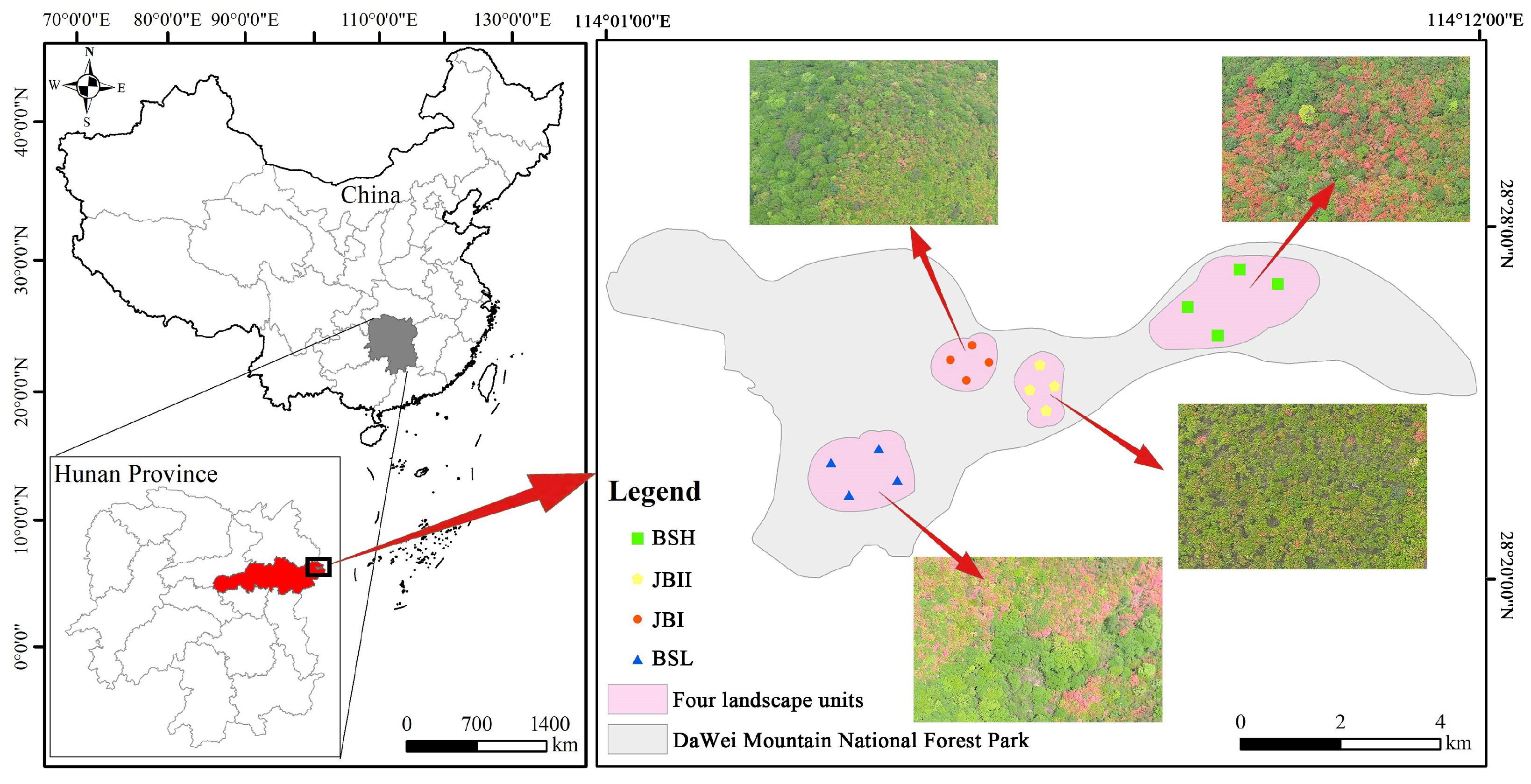
The study area was located in DaWei Mountain National Forest Park, situated in Liuyang City of Hunan Province (28°20^′–28°28^′ N, 114°01^′–114°12^′ E). The topography features erosion of granite landforms at an elevation of 76–2365 m above sea level. The area is characterised by a humid subtropical monsoon climate with an annual average precipitation of 1800–2000 mm and an annual mean air temperature between 11 and 16 ℃ [37,38]. Seasonally, average temperatures range from −4 to 2.5 ℃ in winter (dry season) and from 20 to 28 ℃ in summer (wet season). The soils are mainly developed from granite and mudstone. The soil type exhibits distinct vertical zonation: mountain yellow-brown earth predominates above 1200 m; mountain yellow earth predominates between 800 and 1200 m; and areas below 800 m are characterised by red earth [39].

Regarding land use within the park, the core areas of DaWei Mountain National Forest Park, particularly the mid-to-high elevation zones (above approximately 1200 m) where most of the R. simsii communities occur, are strictly protected and managed for conservation and ecotourism [40]. These areas are dominated by natural forest ecosystems. There are no agricultural activities (crop cultivation) or significant building construction within these core forest zones or specifically within the R. simsii stands targeted by our study [41]. Minor infrastructure associated with tourism (e.g., viewing platforms, trails, small rest stations) exists but was deliberately excluded from our aerial photography sampling locations to focus solely on the natural landscape patterns of the R. simsii colour patches.

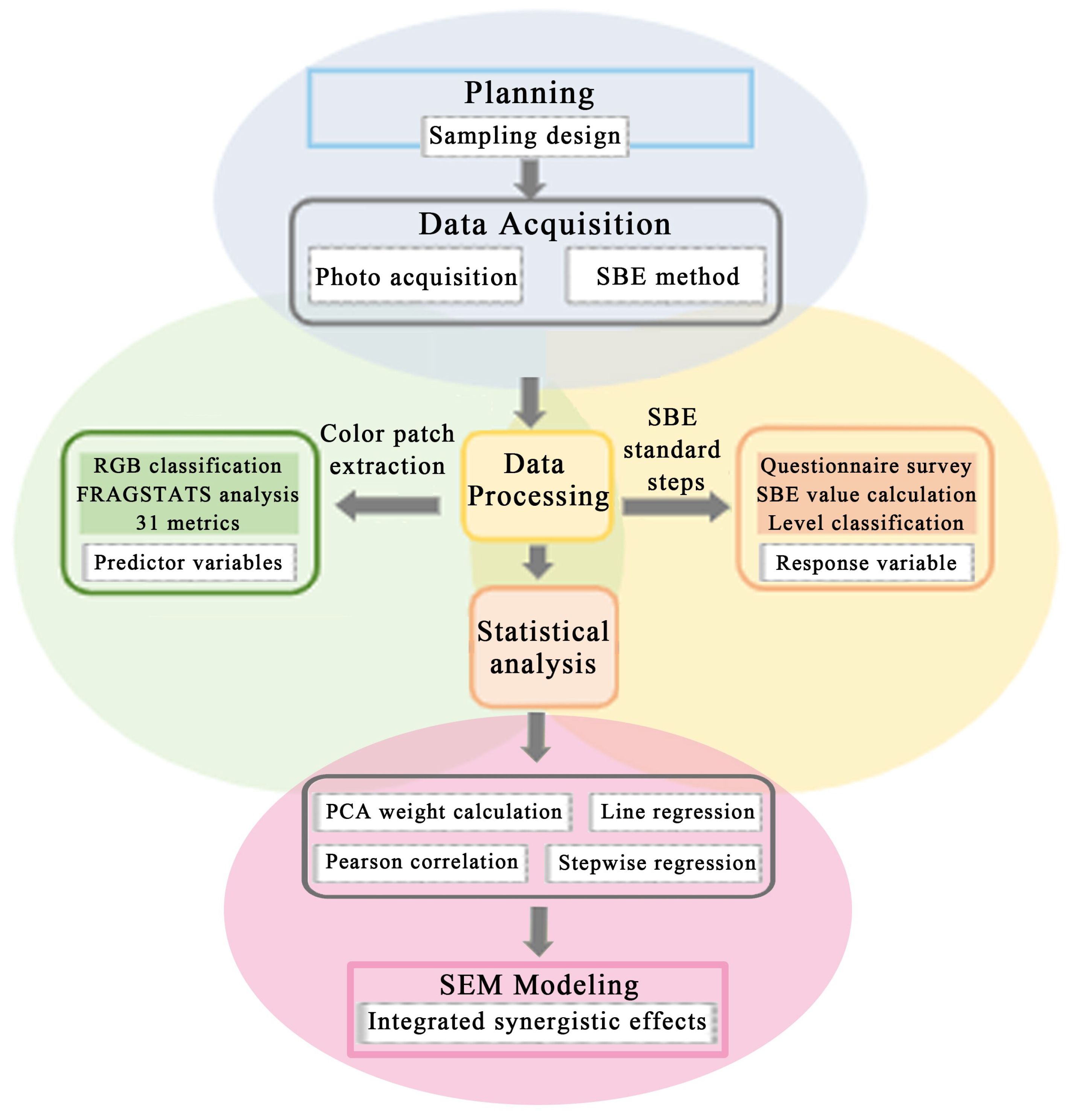
To optimise reader accessibility and scientific reproducibility, our investigation meticulously followed the procedural framework detailed in Figure 1.

2.2. Sampling Design and Photo Acquisition

Four landscape units (Baishihu Flower Sea, Baishilong Flower Sea, and Jiebei Flower Seas I and II) were selected using typical sampling. Within each unit, four 50 m × 50 m replicate plots were systematically positioned based on (1) representative R. simsii coverage; (2) homogeneous topography, and (3) minimum 500 m separation between plots to ensure independence. The 16 plots’ locations and appearance characteristics are shown in Figure 2.

Building upon the established role of maps and aerial imagery as boundary objects in environmental decision-making and participatory planning [42], this study leverages unoccupied aerial vehicles (UAVs/drones) to bridge high-resolution remote sensing and human landscape perception. In May 2021, aerial photographs were taken following standardised forest landscape photography principles [5,43,44]: (1) Non-stand elements were avoided (i.e., roads, equipment); (2) Photographs were taken under sufficient light; (3) Parameters were consistent (DJI Phantom 4 Pro drone at 100 m altitude; nadir orientation; 2.9 cm/pixel resolution).

Sixteen representative photographs (one per plot) were systematically selected from sixty-four candidates through a multi-stage screening protocol that integrated colourimetric analysis and perceptual validation (see Supplementary File S1). The selection adhered to the following criteria:

(1) Exclusion of artificial elements: photographs containing non-vegetation landscape features (i.e., infrastructure, human artifacts) were systematically excluded;

(2) Optimal lighting control: images captured under backlit or side-lit conditions were discarded to ensure consistent illumination;

(3) Illumination consistency: photographs with comparable solar geometry ($\pm {15}^{\circ }$ azimuth) and cloud cover (Okta $\le 2$) were prioritised;

(4) Information richness maximisation: images with low informational value (entropy $<6.0$ bits) were excluded in favour of those optimally representing landscape typologies.

2.3. Colour Patch Extraction

Landscape photographs of distant forest views were processed using Adobe Photoshop to delineate colour patches. Colour calibration was conducted using the X-Rite ColorChecker Passport (mean $\Delta E<1.5$). Ambiguous edges, such as flower–leaf transitions, were manually refined. Visual interpretation served as the primary classification criterion, segregating landscape elements into three chromatic categories based on the following spectral characteristics:

(1) Red patches: Corresponding to flowers of R. simsii (R: 220–255, G: 0–60, B: 0–50);

(2) Green patches: Representing foliage of R. simsii and co-occurring tree species (R: 0–100, G: 90–200, B: 0–120);

(3) Black patches: Denoting shaded tree bases and bare ground (R + G + B < 80, Saturation < 0.1).

Patch classifications were subsequently reclassified in ArcGIS 10.2 (ESRI, Redlands, CA, USA), with automated batch processing via Python ArcPy Module of ArcGIS 10.2. Raster conversion (5 cm resolution) of digitised images enabled quantitative landscape pattern analysis using FRAGSTATS 4.2 [45], extracting key colour patch indices (i.e., patch density, edge complexity).

The landscape indexes were divided into three levels: (1) patch level (processed for individual patches); (2) class level (processed for different types of patches); and (3) landscape level (processed for different land cover classes of patches).

Based on the characteristics of the forest landscape, we selected 31 indicators for analysis: total landscape area (TA), red patch area (RCA), green patch area (GCA), black patch area (BCA), percentage of red patch area (RPLAND), percentage of green patch area (GPLAND), percentage of black patch area (BPLAND), number of patches (NP), patch density (PD), red patch area/green patch area (RCA/GCA), red patch area/black patch area (RCA/BCA), green patch area/black patch area (GCA/BCA), largest patch index (LPI), landscape shape index (LSI), mean patch fractal dimension (FRAC-MN), mean perimeter area ratio (PARA-MN), mean shape index (SHAPE-MN), mean contiguity index (CONTIG-MN), mean related circumscribing circle (CIRCLE-MN), contagion index (CONTAG), path cohesion index (COHESION), landscape division index (DIVISION), perimeter area fractal dimension (PAFRAC), percentage of like adjacencies (PLADJ), Simpson’s evenness index (SIEI), Simpson’s diversity Index (SIDI), Shannon’s diversity Index (SHDI), separation index (SPLIT), Shannon’s evenness index (SHEI), patch richness (PR), and landscape aggregation index (AI). A full list and descriptions are provided in

Table A1. Landscape metrics for colour patch analysis in Rhododendron simsii recreational forests.

Abbr.	Metric Name	Formula	Ecological Interpretation
TA	Total Landscape Area	${\sum }_{i=1}^n{a}_i$	Total area of all patches, indicating landscape extent
RCA	Red Patch Area	$\sum a_{\mathrm{red}}$	Cumulative area of flowering patches (key visual attractor)
GCA	Green Patch Area	$\sum a_{\mathrm{green}}$	Total foliage area (background vegetation dominance)
BCA	Black Patch Area	$\sum a_{\mathrm{black}}$	Area of shaded/bare ground (affects landscape contrast)
RPLAND	Percentage of Red Patch	${\displaystyle \frac{\mathrm{RCA}}{\mathrm{TA}}}\times 100$	Relative dominance of flowering elements
GPLAND	Percentage of Green Patch	${\displaystyle \frac{\mathrm{GCA}}{\mathrm{TA}}}\times 100$	Vegetation coverage proportion
BPLAND	Percentage of Black Patch	${\displaystyle \frac{\mathrm{BCA}}{\mathrm{TA}}}\times 100$	Non-vegetated area proportion
NP	Number of Patches	N	Habitat fragmentation level
PD	Patch Density	${\displaystyle \frac{N}{\mathrm{TA}}}\times 10,000$	Spatial grain of colour distribution
RCA/GCA	Red-Green Area Ratio	${\displaystyle \frac{\mathrm{RCA}}{\mathrm{GCA}}}$	Flower–foliage balance (visual harmony)
RCA/BCA	Red-Black Area Ratio	${\displaystyle \frac{\mathrm{RCA}}{\mathrm{BCA}}}$	Flower–ground contrast intensity
GCA/BCA	Green–Black Area Ratio	${\displaystyle \frac{\mathrm{GCA}}{\mathrm{BCA}}}$	Vegetation–ground contrast
LPI	Largest Patch Index	${\displaystyle \frac{max\left(a_i\right)}{\mathrm{TA}}}\times 100$	Dominance of primary visual focus
LSI	Landscape Shape Index	${\displaystyle \frac{0.25E}{\sqrt{\mathrm{TA}}}}$	Complexity of colour boundaries (E = total edge length)
FRACMN	Mean Fractal Dimension	${\displaystyle \frac{2ln\left(0.25p_i\right)}{ln{a}_i}}$	Geometric intricacy of patch shapes
PARAMN	Mean Perimeter-Area Ratio	${\displaystyle \frac{p_i}{a_i}}$	Edge effect intensity
SHAPEMN	Mean Shape Index	${\displaystyle \frac{p_i}{2\sqrt{\pi a_i}}}$	Deviation from circular form (1 = circle)
CONTIGMN	Mean Contiguity Index	$\left[{\displaystyle \frac{{\sum }_{r=1}^z{c}_{ir}}{z}}\right]{\displaystyle \frac{1}{a_i}}$	Spatial connectedness within patches
CIRCLEMN	Mean Circumscribing Circle	$1-{\displaystyle \frac{a_i}{a_c}}$	Compactness relative to bounding circle ($a_c$ = circle area)
CONTAG	Contagion Index	$\left[1+{\displaystyle \frac{{\sum }_i{\sum }_k{P}_i{g}_{ik}ln\left(P_i{g}_{ik}\right)}{2ln\left(m\right)}}\right]\times 100$	Spatial aggregation of colour classes
COHESION	Patch Cohesion Index	$\left[1-{\displaystyle \frac{\sum p_i}{\sum p_i\sqrt{a_i}}}\right]\times 100$	Physical connectivity of patches
DIVISION	Landscape Division Index	$1-{\sum }_{i=1}^m{\left({\displaystyle \frac{a_i}{\mathrm{TA}}}\right)}^2$	Splitting degree of landscape
PAFRAC	Perimeter-Area Fractal Dim.	${\displaystyle \frac{2}{\beta }}(\beta \mathrm{from}lnp\sim lna)$	Scaling relationship between shape and size
PLADJ	Percentage of Like Adjacencies	${\displaystyle \frac{\sum g_{ii}}{G}}\times 100$	Homogeneity of patch neighbourhood ($g_{ii}$ = like adjacencies)
SIEI	Simpson’s Evenness Index	${\displaystyle \frac{1-\sum P_i^2}{1-1/m}}$	Equitability of colour class distribution
SIDI	Simpson’s Diversity Index	$1-{\sum }_{i=1}^m{P}_i^2$	Probability two random pixels differ in colour
SHDI	Shannon’s Diversity Index	$-{\sum }_{i=1}^m(P_{i}ln{P}_i)$	Richness and evenness of colour classes
SPLIT	Splitting Index	${\displaystyle \frac{{\mathrm{TA}}^2}{{\sum }_{i=1}^n{a}_i^2}}$	Spatial segregation of similar patches
SHEI	Shannon’s Evenness Index	${\displaystyle \frac{-\sum P_{i}ln{P}_i}{lnm}}$	Relative distribution evenness
PR	Patch Richness	m	Number of distinct colour classes

a_i = area of patch i; p_i = perimeter of patch i; P_i = proportion of landscape in class i; m = number of patch classes; n = total number of patches; All metrics computed using FRAGSTATS 4.2 with 5 cm resolution rasters; Colour classes: red (R. simsii flowers), green (R. simsii foliage), black (shaded tree bases/bare ground).

.

2.4. Scenic Beauty Estimation Method

The main work was performed in accordance with standard SBE steps, including a detailed survey of the sample plots, acquisition of forest landscape photographs, selection of landscape evaluation photographs, landscape evaluation, decomposition of landscape elements, data standardisation processing, and establishment of mathematical models. The landscape evaluation method mainly adopted the online questionnaire survey method (guiding participants to operate from a computer or mobile phone by posting a link) to obtain universal aesthetic standards of the evaluator [9,15]. Several studies have shown that there is no statistical difference in the aesthetic senses of different evaluation subjects [46,47,48]. Professional and non-professional group assessors are consistent in making aesthetic evaluations of plant communities, but the professional group exhibits a greater sensitivity to the aesthetics of the plant community [49]. To ensure the objectivity and accuracy of the evaluations, we selected a total of 1549 participants, mainly graduate students and some social workers majoring in relevant subjects in school. This study involving human participants was conducted in accordance with institutional guidelines and the National Ethical Review Regulations for Non-Biomedical Research (Article 17, 2021). Formal ethics committee approval was waived as this study (1) exclusively employed anonymous questionnaire surveys; (2) involved no clinical interventions or sensitive data collection; (3) posed minimal risk (Category A per CIOMS Guidelines). All participants provided written informed consent in compliance with the Declaration of Helsinki (2013) [50]. The survey protocols ensured (1) confidentiality, as data were anonymised through participant ID coding; (2) voluntary participation, with the option to withdraw without penalty; (3) privacy protection, as secure storage was used, per GDPR Article 32.

The specific process was as follows [14,51,52]:

(1) Participants electronically signed informed consent documentation confirming their voluntary participation before the study commenced.

(2) Survey objectives and scoring criteria were introduced, and all 16 photographs were previewed to establish perceptual baselines.

(3) Photographs were displayed individually in fixed sequence with a fixed display duration (60 s per image). The beauty of the landscape was scored using a 7-point Likert scale to represent the degree of scenic appeal: very like (3), like (2), slightly like (1), neutral (0), slightly dislike (−1), dislike (−2), and very dislike (−3).

(4) All participants were counted after the evaluation, and disqualified questionnaires (duplicate submissions and incomplete responses) were removed. Then, the beauty value of each landscape photo was counted according to the calculation method.

The complete survey instrument is provided as Supplementary File S1, featuring the informed consent form, survey questionnaire, and statistical analysis report.

2.5. Data Statistical Analysis

2.5.1. Predictor Variables: Colour Patch Metrics

The 31 colour patch metrics served as predictor variables.

Min–max normalisation method. We adopted min–max normalisation to standardise the raw data. This is a classical data processing and pre-processing technique which can convert the data to the ratio between the original values [53] calculated by Equation (1).

$$x^{\prime }={\displaystyle \frac{x-x_{Min}}{x_{Max}-x_{Min}}}$$

(1)

where x represents the original data; $x_{\begin{array}{c}Max\end{array}}$ and $x_{Min}$, respectively, represent the maximum and minimum values in the original data group of the same indicator; and $x^{\prime }$ represents the standardised data.

Weight calculation of colour patch indicators. After data standardisation, principal component analysis was used to determine the weights of colour patch indicators and was calculated by Equations (2) and (3).

$$M={\displaystyle \frac{{\sum }_{i=1}^m\frac{L_i{V}_j}{\sqrt{E_j}}}{{\sum }_{j=1}^n{V}_j}}$$

(2)

$$w={\displaystyle \frac{\overline{M_i}}{{\sum }_{i=1}^m\overline{M_i}}}$$

(3)

where m represents the extraction number of colour patch indicators; $L\begin{array}{c}i\end{array}$ represents the load value of the i-th indicator of the j-th principal component; $E\begin{array}{c}j\end{array}$ represents the eigenvalue of the j-th principal component; $V\begin{array}{c}j\end{array}$ represents the variance (%) of the j-th principal component; M represents the coefficient in the comprehensive score model of n principal components; $\overline{M\begin{array}{c}i\end{array}}$ represents the standardisation coefficient in the principal component composite score model treated by min–max normalisation (Equation (1)); and w represents the weight of the i-th indicator in the colour patch extraction index. Due to the possibility of negative load values for each indicator in principal component analysis, M may have negative values. According to the 3$\sigma$ criterion, the coordinate translation method was used to shift the M values of all indicators to the right by 1 to eliminate the influence of negative numbers, facilitating weight calculation and the next step in the analysis.

2.5.2. Response Variable: Scenic Beauty Estimation

$\mathbf{Beauty}\mathbf{value}\mathbf{calculation}$. The SBE method standardising equation was used to standardise the rating scores of each photo from 1538 people in the evaluation questionnaire, calculate the average standardised score (Z value) for each sample photo, and further calculate the SBE scores of the sample land. The calculation was carried out using Equations (4) and (5).

$$Z_{ij}=(R_{ij}-\overline{R})/S_j$$

(4)

$$S_i=\sum _{j=1}^{N_i}{Z}_{ij}/N_i$$

(5)

where $R\begin{array}{c}ij\end{array}$ represents the rating value of the j-th survey object on the i-th landscape; $\overline{R}$ represents the average of all scoring values for the j-th survey object; $S\begin{array}{c}j\end{array}$ represents the standard deviation of all scoring values for the j-th survey object; $Z\begin{array}{c}ij\end{array}$ represents the standardised score obtained by the j-th survey object for the i-th landscape; $N\begin{array}{c}i\end{array}$ represents the number of personnel participating in the i-th landscape evaluation; and $S\begin{array}{c}i\end{array}$ is the final SBE score for the i-th landscape.

$\mathbf{Beauty}\mathbf{level}\mathbf{classification}$. Scenic beauty was divided into five levels using the equal difference method [54]: the first grade is very good (VI), the second is good (IV), the third is average (III), the fourth is poor (II), and the fifth is very poor (I). The specific calculation equations are shown in

Table 1. The calculation equations of the grade division in the assessment of scenic beauty.

Grade	Minimum Value	Maximum Value
VI	(SBE$\begin{array}{c}max\end{array}$ − SBE$\begin{array}{c}min\end{array}$) × 80% + SBE$\begin{array}{c}min\end{array}$	(SBE$\begin{array}{c}max\end{array}$ − SBE$\begin{array}{c}min\end{array}$) + SBE$\begin{array}{c}min\end{array}$
IV	(SBE$\begin{array}{c}max\end{array}$ − SBE$\begin{array}{c}min\end{array}$) × 60% + SBE$\begin{array}{c}min\end{array}$	(SBE$\begin{array}{c}max\end{array}$ − SBE$\begin{array}{c}min\end{array}$) × 80% + SBE$\begin{array}{c}min\end{array}$
III	(SBE$\begin{array}{c}max\end{array}$ − SBE$\begin{array}{c}min\end{array}$) × 40% + SBE$\begin{array}{c}min\end{array}$	(SBE$\begin{array}{c}max\end{array}$ − SBE$\begin{array}{c}min\end{array}$) × 60% + SBE$\begin{array}{c}min\end{array}$
II	(SBE$\begin{array}{c}max\end{array}$ − SBE$\begin{array}{c}min\end{array}$) × 20% + SBE$\begin{array}{c}min\end{array}$	(SBE$\begin{array}{c}max\end{array}$ − SBE$\begin{array}{c}min\end{array}$) × 40% + SBE$\begin{array}{c}min\end{array}$
I	SBE$\begin{array}{c}min\end{array}$	(SBE$\begin{array}{c}max\end{array}$ − SBE$\begin{array}{c}min\end{array}$) × 20% + SBE$\begin{array}{c}min\end{array}$

SBE: the final score of scenic beauty estimation.

.

$\mathbf{Statistical}\mathbf{analysis}$. For data standardisation, to determine the average value and other routine calculations, we used the Microsoft Excel package. All statistical analyses were conducted using the R statistical software 4.4.3 package [55]. Principal component analysis (extraction of SBE influence factor (colour patch indicators) and weight calculation) was implemented using the $FactoMineR$ package [56] and visualised using the $factoextra$ [57] and $ggplot2$ packages [58] of the R software. A Pearson correlation plot (correlation between SBE values and indicators of colour patches) was drawn using the $Corrplot$ package [59] in the R statistical software. The comprehensive weight value of colour patch traits of the landscapes was plotted using the $tidyverse$ [60], $reshape2$ [61], $ggplot2$ [58], and $ggprism$ [62] packages in R. Based on the results of the principal component and Pearson correlation analyses, we used linear function analysis to further examine the trend in key colour patch element indicators changing with the beauty grade. The figure of linear function analysiswas produced via the $ggplot2$ [58], $tidyverse$ [60], and $dplyr$ [63] packages in R. Following the principal component analysis, we conducted stepwise regression analysis to determine the leading impact factors for the SBE values. This analysis was performed using the step function of R statistical software. Structural equation modelling (SEM) was performed using the $piecewiseSEM$ package [64] in R to further examine the synergistic effects of the area percentage, shape, and space collocation of colour patches on the SBE. The figure of SEM analysiswas plotted by the $ggplot2$ [58], and $patchwork$ [65] packages of R.

3. Results

3.1. Selection of Colour Patch Indicators for R. simsii Landscape Recreational Forest

The indicator features extracted from the colour patches varied among different units evaluated (

Table 2. Colour patch indicators of different evaluated landscape units (mean ± SD).

Indicators	BSH	BSL	JBI	JBII
TA	1083.80 ± 0.00	1986.13 ± 0.00	1992.29 ± 0.00	1996.54 ± 0.00
RCA	301.00 ± 53.07	257.15 ± 58.58	86.93 ± 32.33	87.70 ± 53.05
GCA	749.22 ± 37.49	1663.26 ± 39.72	1847.54 ± 45.94	1698.48 ± 175.39
BCA	33.59 ± 19.83	75.77 ± 42.38	61.71 ± 20.95	210.01 ± 197.80
RPLAND	27.77 ± 4.90	12.95 ± 2.93	4.36 ± 1.62	4.39 ± 2.66
GPLAND	69.13 ± 3.46	83.74 ± 1.99	92.73 ± 2.30	85.07 ± 8.79
BPLAND	3.10 ± 1.83	3.31 ± 2.12	2.90 ± 1.05	10.49 ± 9.91
RCA/GCA	0.40 ± 0.09	0.15 ± 0.04	0.05 ± 0.02	0.05 ± 0.03
RCA/BCA	8.96 ± 15.44	3.91 ± 6.63	1.50 ± 0.66	0.42 ± 18.31
GCA/BCA	22.30 ± 29.03	25.31 ± 29.85	31.95 ± 11.66	8.11 ± 207.63
NP	7925.25 ± 1987.77	13,660.50 ± 7608.15	7598.75 ± 3334.77	6346.75 ± 4350.16
PD	731.25 ± 183.41	684.33 ± 381.13	380.66 ± 167.06	317.94 ± 217.92
LPI	64.69 ± 4.32	81.24 ± 2.12	91.69 ± 2.74	83.29 ± 9.96
LSI	38.96 ± 5.07	44.66 ± 12.50	26.39 ± 9.63	32.02 ± 17.46
SHAPE-MN	1.31 ± 0.06	1.34 ± 0.04	1.37 ± 0.03	1.39 ± 0.05
FRACMN	1.17 ± 0.01	1.17 ± 0.00	1.18 ± 0.01	1.16 ± 0.01
PARA-MN	19,256.29 ± 3821.95	17,516.65 ± 2241.31	16,771.40 ± 307.57	16,010.66 ± 1969.91
CIRCLE-MN	0.45 ± 0.04	0.47 ± 0.02	0.49 ± 0.01	0.46 ± 0.01
CONTIG-MN	0.48 ± 0.10	0.53 ± 0.06	0.54 ± 0.01	0.57 ± 0.05
PAFRAC	1.25 ± 0.02	1.27 ± 0.01	1.28 ± 0.01	1.22 ± 0.01
CONTAG	62.56 ± 1.78	71.47 ± 1.82	83.18 ± 4.31	75.82 ± 10.01
PLADJ	97.66 ± 0.31	98.02 ± 0.56	98.84 ± 0.43	98.59 ± 0.78
COHESION	99.94 ± 0.00	99.95 ± 0.01	99.96 ± 0.00	99.96 ± 0.01
DIVISION	0.57 ± 0.05	0.34 ± 0.03	0.16 ± 0.05	0.30 ± 0.16
SPLIT	2.35 ± 0.27	1.52 ± 0.08	1.19 ± 0.07	1.49 ± 0.39
PR	3.00 ± 0.00	3.00 ± 0.00	3.00 ± 0.00	3.00 ± 0.00
SHDI	0.71 ± 0.03	0.53 ± 0.05	0.31 ± 0.08	0.46 ± 0.18
SIDI	0.44 ± 0.02	0.29 ± 0.03	0.14 ± 0.04	0.25 ± 0.12
SHEI	0.65 ± 0.03	0.48 ± 0.04	0.28 ± 0.07	0.42 ± 0.17
SIEI	0.66 ± 0.04	0.43 ± 0.04	0.21 ± 0.06	0.37 ± 0.19
AI	97.71 ± 0.31	98.06 ± 0.56	98.87 ± 0.43	98.62 ± 0.78

BSH: Baishihu Flower Sea; BSL: Baishilong Flower Sea; JBI: Jiebei Flower Sea I; JBII: Jiebei Flower Sea II; TA: total landscape area; RCA: red patch area; GCA: green patch area; BCA: black patch area; RPLAND: percentage of red patch area; GPLAND: percentage of green patch area; BPLAND: percentage of black patch area; NP: number of patches; PD: patch density; RCA/GCA: red patch area/green patch area; RCA/BCA: red patch area/black patch area; GCA/BCA: green patch area/black patch area; LPI: largest patch index; LSI: landscape shape index; FRAC-MN: mean patch fractal dimension; PARA-MN: mean perimeter area ratio; SHAPE-MN: mean shape index; CONTIG-MN: mean contiguity index; CIRCLE-MN: mean related circumscribing circle; CONTAG: contagion index; COHESION: path cohesion index; DIVISION: landscape division index; PAFRAC: perimeter area fractal dimension; PLADJ: percentage of like adjacencies; SIEI: Simpson’s evenness index; SIDI: Simpson’s diversity Index; SHDI: Shannon’s diversity Index; SPLIT: separation index; SHEI: Shannon’s evenness index; PR: patch richness; AI: landscape aggregation index.

). There were significant differences in the changes among 21 indicators, including RCA, GCA, BCA, RPLAND, GPLAND, BPLAND, NP, PD, RCA/GCA, RCA/BCA, GCA/BCA, LSI, LPI, PARA-MN, DIVISION, CONTAG, SPLIT, SHDI, SHEI, SIDI, and SIEI. The results showed that the gradient division of the selected evaluated landscape units was reasonable, and the evaluation of their beauty was of scientific significance.

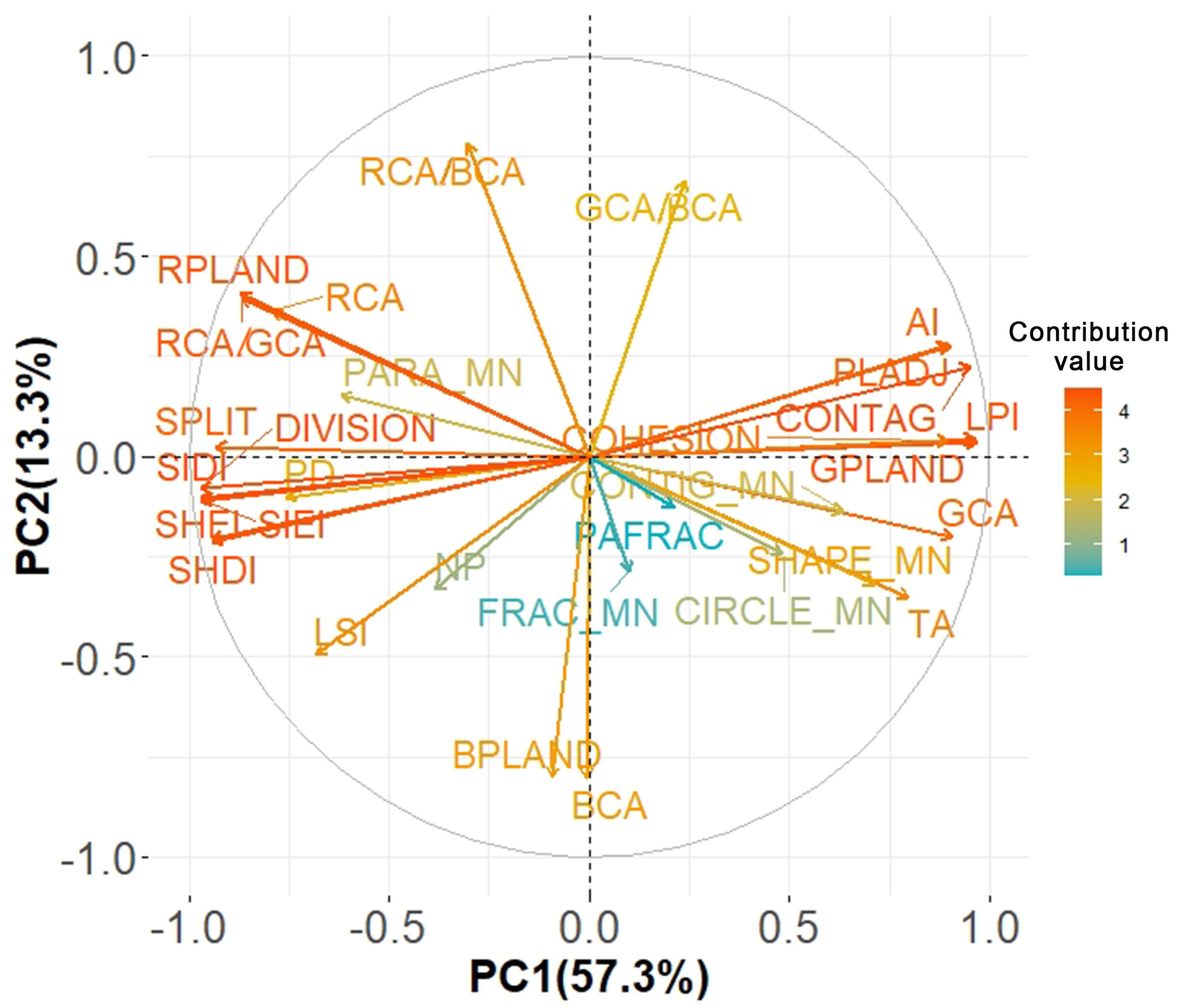
Based on the two indicators of eigenvalues (>1) and the cumulative contribution rate (>85%), five principal components were selected. The indicator with an absolute loading matrix value > 0.7 was selected as the dominant factor [66] for the selection criteria. The results showed that the colour patch indicators accounted for 94.8% of the variation in landscape features in far-distance images of the forest. The first principal component can be summarised as the colour characteristics of patches, reflecting the size, distribution percentage, heterogeneity, and aggregation of the landscape colour patches. There were 19 indicators, including TA, RCA, GCA, RPLAND, GPLAND, RCA/GCA, PD, SHAPE-MN, CONTAG, LPI, COHESION, DIVISION, PLADJ, SPLIT, SIDI, SHDI, SIEI, SHEI, and AI. The second principal component reflected the distribution ratio of red and black patches in the landscape. A total of three indicators were extracted: BCA, BPLAND, and RCA/BCA. The third principal component mainly referred to the overall distribution of the landscape pattern, including NP, FRAC-MN, and PAFRAC. There were no main factors extracted from the fourth and fifth principal components (Figure 3).

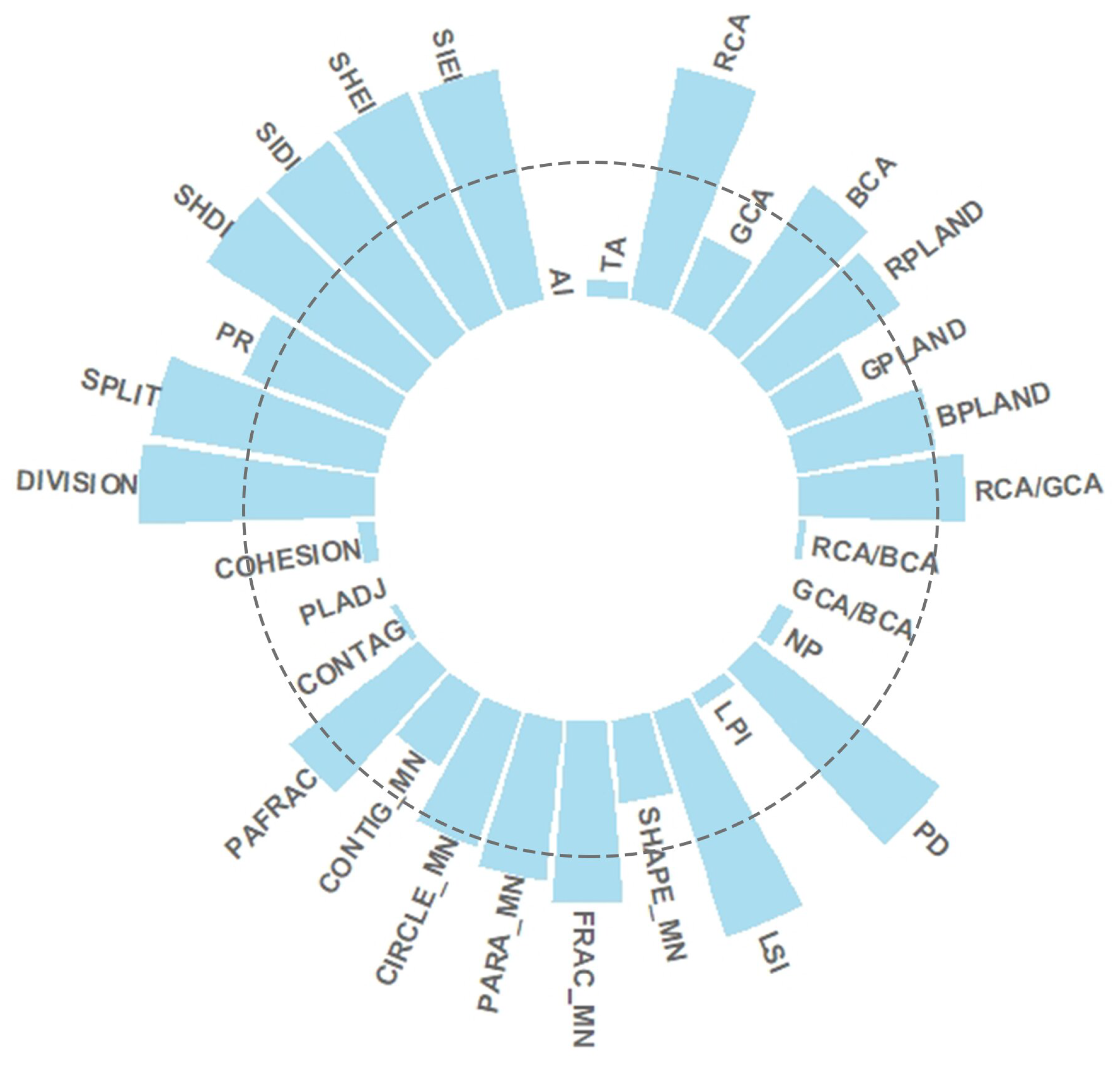
According to the selection criteria of indicators with comprehensive weight values > 0.032 (1/31), there were 19 indicators selected for the next analysis: RCA, BCA, RCA/GCA, RPLAND, BPLAND, PD, CIRCLE-MN, LSI, NP, FRAC-MN, PAFRAC, PARA-MN, DIVISION, SHDI, SHEI, SPLIT, PR, SIDI, and SIEI (Figure 4).

3.2. Overall Beauty Evaluation of R. simsii Landscape Recreational Forest

The calculation results showed that the degree of beauty of the R. simsii landscape recreational forest was divided into five levels: very good, good, average, poor, and very poor (

Table 3. The grade division in the assessment of scenic beauty for $\mathit{Rhododendron\; simsii}$ forest landscapes in the far-distance view.

Grade	SBE Minimum Value	SBE Maximum Value	Evaluation Level
VI	0.60	1.02	very good
IV	0.18	0.60	good
III	−0.24	0.18	average
II	−0.66	−0.24	poor
I	−1.08	−0.66	very poor

SBE: the final score of scenic beauty estimation.

). The results of the scenic beauty score revealed that the four landscape units of Baishihu Flower Sea had high scenic beauty, and all of them reached good or very good levels. The visual quality levels of the four landscape units of Baishilong Flower Sea were mainly poor, average, or good. All landscape units of Jiebei Flower Sea I had visual quality showing poor or average levels. The visual quality of the four landscape units of Jiebei Flower Sea II had the lowest values, which were very poor, poor, or average (

Table 4. Scenic beauty scores of different evaluated landscape units.

Landscape Units	Average Scores	Standardised Scores	Evaluation Levels
BSH1	2.12	1.02	very good
BSH2	1.66	0.59	good
BSH3	2.05	0.95	very good
BSH4	1.67	0.68	very good
BSL1	0.74	−0.27	poor
BSL2	1.45	0.43	good
BSL3	0.66	−0.35	poor
BSL4	0.78	−0.21	average
JBI1	0.92	−0.07	average
JBI2	0.90	−0.12	average
JBI3	0.95	−0.04	average
JBI4	0.64	−0.34	poor
JBII1	1.09	0.05	average
JBII2	0.35	−0.65	poor
JBII3	0.34	−0.59	poor
JBII4	−0.19	−1.08	very poor

BSH: Baishihu Flower Sea; BSL: Baishilong Flower Sea; JBI: Jiebei Flower Sea I; JBII: Jiebei Flower Sea II.

).

3.3. The Dominant Factors Affecting the Scenic Beauty of $\mathit{Rhododendron}\mathit{simsii}$ Landscape Recreational Forests

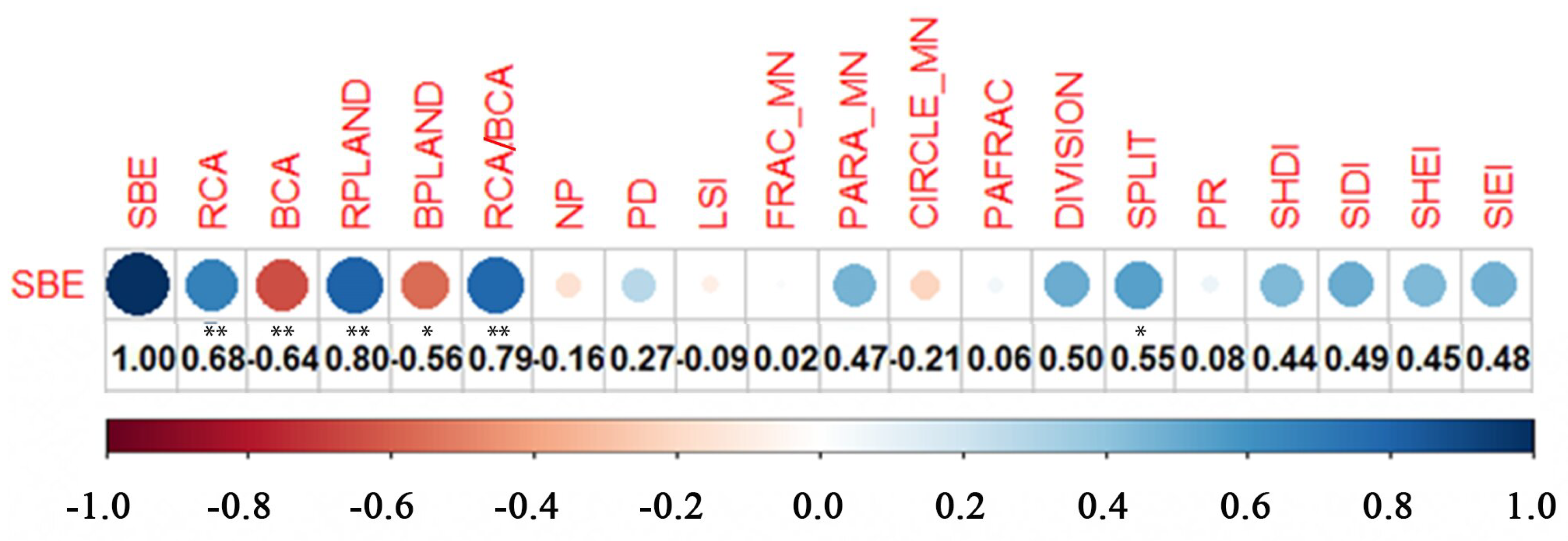
The results of the Pearson correlation analysis (Figure 5) indicated that the SBE value of the R. simsii landscape recreational forests was significantly or extremely significantly positively correlated with RCA, RPLAND, RCA/BCA, and SPLIT ($\mathit{p}$ < 0.05). There was a remarkable or extremely remarkably negative correlation between the SBE value and BCA and BPLAND ($\mathit{p}$ < 0.05). Specifically, the SBE value strongly correlated with RPLAND and RCA/BCA, with correlation coefficients of 0.80 and 0.79, respectively.

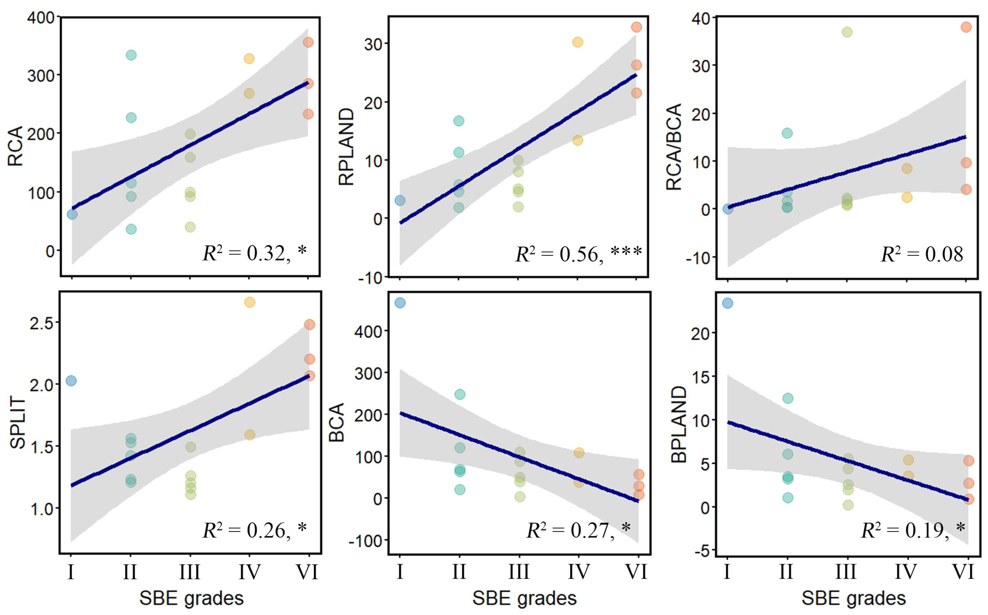
Following the results of the Pearson correlation analysis, we conducted a linear regression analysis to assess the relationships between the SBE grades and key colour patch indicators (Figure 6). The SBE grades significantly increased with RCA, RPLAND, and SPLIT, whereas they decreased remarkably with BCA and BPLAND.

The synergistic influence mechanism of various factors on the visual quality of R. simsii landscape recreational forests cannot be fully clarified by analysing the role of individual indicators alone. To reveal the relative importance of each colour patch indicator for the aesthetic value, a stepwise regression analysis was conducted on the indicators with high weight values obtained from the principal component analysis, and the final key factors were determined (

Table 5. Stepwise regression analysis of influencing factors of the SBE value.

Model	Indicators	Non-Standardised Coefficient	${\mathit{R}}^2$	p
1	Constant	−0.569	0.802	<0.05
	RPLAND	0.046
2	Constant	0.038	0.902	<0.05
	RPLAND	0.056
	LSI	−0.020
3	Constant	−0.912	0.932	<0.05
	RPLAND	0.050
	LSI	−0.024
	PARA-MN	0.001

$R^2$: model adjustment judgment coefficient; p: the significance level of simulation effect.

). The highest adjustment coefficient ($R^2$) was found for model 3, and the simulation effect reached a significant level ($\mathit{p}$ < 0.01). The regression equation was as follows: ySBE = 0.050x$\begin{array}{c}RPLAND\end{array}$ – 0.024x$\begin{array}{c}LSI\end{array}$ + 0.001x$\begin{array}{c}PARA-MN\end{array}$ – 0.912. The results show that the variation in SBE value was due to the comprehensive effect of RPLAND, LSI, and PARA-MN.

3.4. Synergy Effects of Landscape Indicators on the Variation in SBE of the R. simsii Landscape Recreational Forests

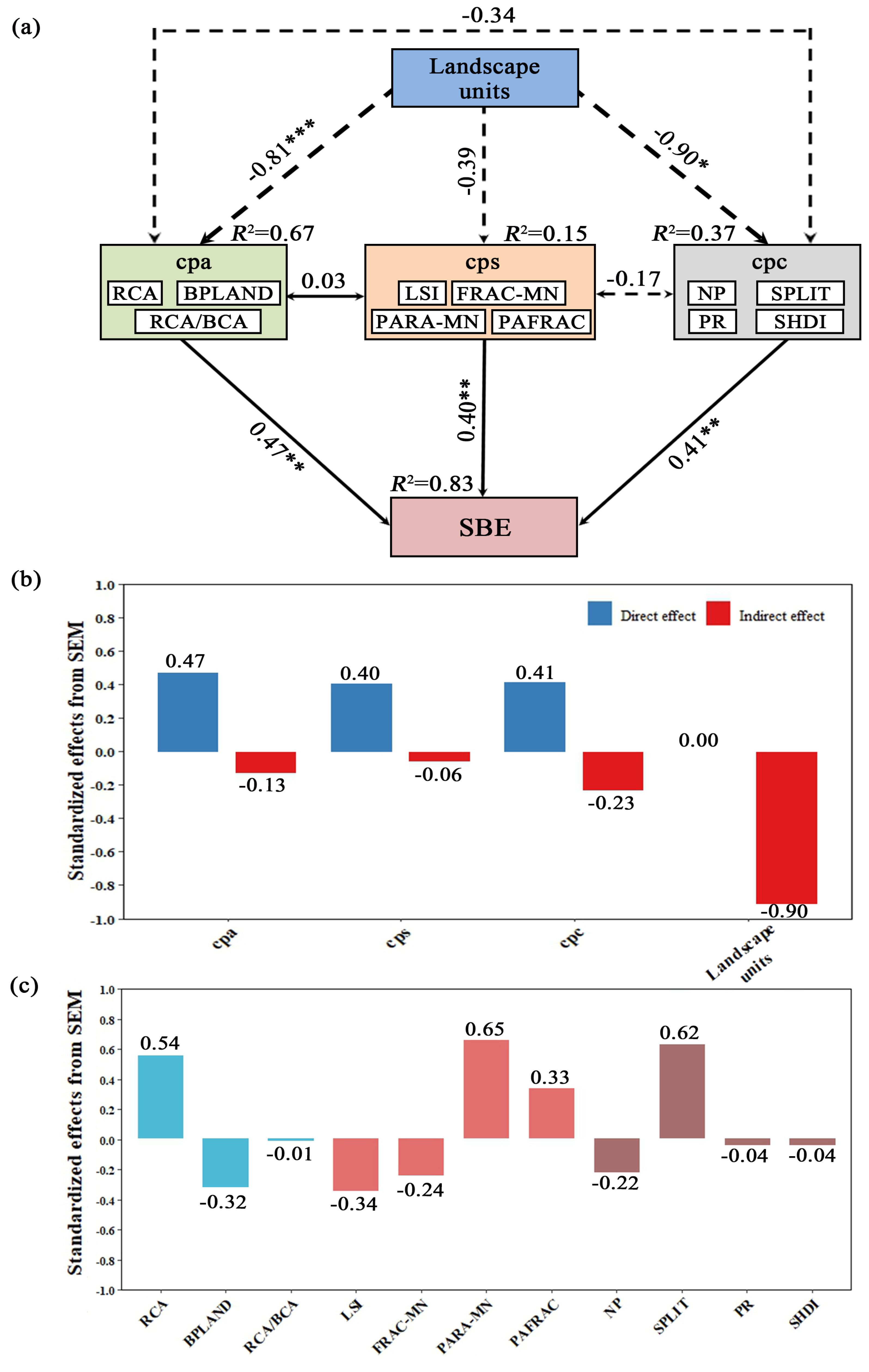
To elucidate the integrated synergistic effects of landscape indicators on the SBE values of the R. simsii landscape recreational forests and identify latent variable factors, we developed an SEM framework (Figure 7). Based on the functional–structural properties of the landscape indicators, they were categorised into three distinct groups: the area percentage of colour patches (cpa, including RCA, BPLAND and RCA/BCA), the shape of the colour patches (cps, including LSI, FRAC-MN, PARA-MN and PAFRAC), and the space collocation of colour patches (cpc, including NP, SPLIT, PR and SHDI). The results of this model showed no significant deviation from the observed data, thereby supporting adequate model fit, as indicated by residual normality analysis (Shapiro–Wilk test, W = 0.98, $\mathit{p}$ = 0.48), the Akaike Information Criterion (AIC = 45.08), tests of directed separation ($\mathit{p}$ = 0.41), global goodness-of-fit tests (Chi-Squared = 1.01, $\mathit{p}$ = 0.31) and Fisher’s C test (C = 1.76, $\mathit{p}$ = 0.41, degrees of freedom [df] = 11) [67,68]. This non-significant p-value ($\mathit{p}$ > 0.05) aligns with established thresholds for SEM, where higher $\mathit{p}$-values reflect better alignment between theoretical constructs and empirical covariance structures [69].

The SEM demonstrated robust explanatory capacity for the variation in SBE values, with $R^2$ = 0.83 (Figure 7a), indicating that 83% of the variance in SBE values was accounted for by the integrated landscape indicators. The area percentage of colour patches (cpa), shape of colour patches (cps), and space collocation of colour patches (cpc) exhibited strong positive direct effects on SBE, with coefficients of 0.47, 0.40, and 0.41, respectively (Figure 7b). The heterogeneity in SBE values across landscape units was predominantly mediated by negative indirect effects stemming from three distinct groups of landscape indicators, with coefficients of −0.90 (Figure 7b). Furthermore, RCA, PARA-MN, and SPLIT were identified as critical latent variables driving variations in SBE values. These indicators exerted significant positive standardised effects on SBE values, with path coefficients of 0.54, 0.65, and 0.62, respectively (Figure 7c).

4. Discussion

4.1. Regulatory Mechanisms of Colour Patch Dynamics and Spatial Heterogeneity on Far-Distance Visual Quality in $\mathit{R}.\mathit{simsii}$ Landscape Recreational Forests

Consideration of visual aesthetics outside the forest includes analysis and research on the distribution pattern and landscaping of plant landscapes, landscape colour matching, spatial hierarchy, landscape diversity, and colour richness. Changes in landscape pattern significantly affect various ecological processes and regulate the aesthetic characteristics of landscape visual elements. Specifically, landscape colour had a strong impact on people’s visual behaviour and preferences [25,36]. The higher the colour diversity of the patches, the stronger the colour contrast of the patches and the clearer the visual impact, which aligns better with people’s psychological need for diversity, change, and richness [28]. The results of Mu et al. (2022) [52] showed that forests with superior visual aesthetic quality had more obvious colour contrast and diverse colours with primary and secondary contrast. Our results showed that the main landscape colour patch characteristics of the R. simsii landscape recreational forests were represented by the colour patch quality index, which indicated that the landscape quality in far-distance views of forests is closely related to the colour patch quality. Additionally, the areas and proportional distribution of different patches were dominant factors in the variation in scenic beauty. In our study, an increase in the area and percentage of red patches, a decrease in the area and percentage of black patches, and a significant increase in the ratio of red to black patch areas ultimately enhanced the scenic beauty of the R. simsii landscape recreational forests in far-distance views. These results are consistent with our hypothesis that the mechanism of colour patch dynamics and spatial heterogeneity synergistically promotes landscape visual quality. These results were consistent with other research that found that an increase in red patches improved visual aesthetic quality [29], further confirming that a landscape rich with colours can give people a better visual experience than a single-colour landscape [30,70,71]. Therefore, it is recommended to increase the percentage and coverage of R. simsii species in black patch areas with low scenic beauty, such as Baishilong Flower Sea and Jiebei Flower Seas I and II, via replanting [72], further enhancing the visual impact of the main colour patches and improving the aesthetic experience of visitors.

This study also found that SPLIT, LSI, and PARA-MN were key factors affecting the beauty of R. simsii in far-distance views of the landscape recreational forests. As SPLIT increased, patch distribution can become more dispersed, and patch number and density can be higher, which is conducive to improving colour diversity and contrast. Meanwhile, with the decline in LSI and PARA-MN, patch shape showed a more regular and simple trend, which could reduce clutter in the landscape layout. These results also offer further evidence for the hypothesis that landscape visual quality in far-distance views of R. simsii landscape recreational forests is affected by the shape of colour patches. As a consequence, our research proposes the following suggestions: (1) changes in spatial depth can be realised by increasing the dispersion of patches and rationally arranging the spatial collocation of patches with different colours and (2) visual field barriers affecting the view of R. simsii should be properly cleared, and other tree species affecting the edge layout should be pruned and thinned [73].

In summary, according to existing resources of the wild genus $\mathit{Rhododendron}$, for protection and breeding, introducing new varieties combined with the characteristics of the original genus $\mathit{Rhododendron}$ is recommended. The adjacent arrangement of related species would be helpful in increasing thhe ornamental highlights of R. simsii in the forest and enriching the structure of the R. simsii community.

4.2. Comprehensive Regulatory Effect of Key Landscape Indicators on Aesthetic Quality of R. simsii Landscape Recreational Forests

The comprehensive evaluation of landscape quality necessitates integrating the interactions between natural attributes and human perceptual responses [2]. In this study, a SEM framework was employed to elucidate the integrated synergistic effects of landscape indicators on the SBE values of R. simsii landscape recreational forests. The SEM demonstrated robust explanatory capacity, accounting for 83% of the variance in SBE values ($R^2$ = 0.83), which underscores the critical role of colour patch area percentage (cpa), patch shape complexity (cps), and spatial configuration (cpc) as core determinants of landscape aesthetic quality. These results provide empirical support for the hypothesis that the synergistic interplay of colour patch area percentage, shape attributes, and spatial collocation jointly enhances the visual quality of R. simsii recreational forests. This high explanatory power aligns with previous studies emphasising the multidimensional drivers of aesthetic preferences [2,3], further reinforcing the comprehensive regulatory role of landscape indicators on visual perception.

The direct effect coefficients of CPA, CPS, and CPC on SBE were 0.47, 0.40, and 0.41, respectively, aligning with findings from autumn landscape evaluations in Saihanba National Forest Park, where dominant chromatic attributes and shape complexity contributed 30 75% of the variance in SBE [74]. This consistency highlights the pivotal role of colour diversity and spatial hierarchy richness in optimising landscape aesthetics. RCA (path coefficient = 0.54), PARA-MN (path coefficient = 0.65), and SPLIT (path coefficient = 0.62) emerged as critical latent variables exerting positive effects on SBE values by enhancing the dominance of primary chromatic attributes, patch coherence, and morphological complexity, respectively. These findings align with conventional hypotheses regarding the benefits of patch size optimisation in landscape aesthetics [22]. Conversely, the negative impacts of LSI (path coefficient = −0.34) and FRAC-MN (path coefficient = −0.24) on SBE suggest that excessive geometric complexity and shape irregularity of patches may diminish landscape aesthetic quality. This implies that overly intricate spatial patterns could overwhelm human visual processing, thereby reducing aesthetic appeal. These observations are consistent with prior findings that fragmented patches or excessive spatial heterogeneity induce visual disintegration, impairing the perceptual coherence of landscapes [75].

The study provides definitive optimisation pathways for the landscape design of R. simsii landscape recreational forests: (1) augmenting visual appeal by increasing the proportion of high-saturation patches (i.e., clustered flowering plants), which amplifies chromatic salience and focal attraction; (2) avoiding excessive geometric complexity (i.e., high FRAC-MN values) and adopting moderate fractal dimension designs with natural curvatures to balance aesthetic and ecological functionality; and (3) reducing patch dispersion (lower SPLIT index) to enhance core area coherence, thereby improving visual continuity and ecological stability.

4.3. Methodological Considerations and Future Directions

While this study provides novel insights into colour-patch-driven aesthetics, several methodological aspects warrant further consideration. (1) Our findings are specific to far-distance viewing contexts. Future research should establish distance–decay functions to quantify how aesthetic responses shift across viewing scales, particularly for mid-range and proximate perspectives. This could be achieved through multi-scale UAV surveys coupled with eye-tracking validation. (2) This study captured colour patterns during peak flowering (May), but aesthetic value fluctuates seasonally. Longitudinal monitoring using phenocams or monthly UAV surveys could reveal how colour patch metrics influence aesthetic perception across phenological stages. (3) Our evaluator cohort consisted primarily of Chinese graduate students and some social workers. Cross-cultural validation with diverse demographic groups (i.e., European or North American cohorts) and age profiles would strengthen the universal applicability of our models. (4) While UAV-derived metrics effectively capture 2D spatial patterns, they cannot quantify the 3D structural complexity that influences light interception and colour saturation. Integrating terrestrial LiDAR with hyperspectral sensors would better characterise the vertical dimension of colour expression.

5. Conclusions

This study provides conclusive evidence that the spatial configuration of colour patches, particularly those formed by $\mathit{Rhododendron\; simsii}$, is a primary driver of far-distance scenic beauty in recreational forests, which is effectively quantifiable through a combination of the SBE method and landscape pattern analysis. We conclusively demonstrated that far-distance visual quality was not merely subjective but could be robustly predicted by measurable spatial metrics of colour patches. The area percentage, shape complexity, and spatial distribution pattern of these patches collectively explained the vast majority of variance in perceived scenic beauty. This provided a strong mechanistic understanding of how specific, modifiable landscape features govern aesthetic responses at a distance. This study reveals that aesthetic quality arises from the synergistic interplay of key patch attributes. Optimal scenic beauty was achieved not by maximising any single metric but through a combination of (1) a dominant chromatic presence (particularly red hues), enhancing visual salience; (2) moderately complex fractal-like shapes, contributing to visual richness and coherence; and (3) reduced spatial dispersion (increased aggregation), promoting a sense of order and pattern integrity. Neglecting any of these dimensions could diminish the overall aesthetic value. Our findings translate directly into actionable strategies for enhancing the visual quality of R. simsii recreational forests and similar ecosystems. Managers and designers should implement interventions that (1) prioritise the conservation of large contiguous flowering patches to strengthen chromatic impact; (2) maintain or introduce moderate shape complexity within patches to avoid monotony without creating visual chaos; and (3) manage the spatial arrangement to encourage patch aggregation, reducing fragmentation and enhancing the perceived scale and coherence of the colour display. The successful application of SEM confirmed its power in disentangling the complex, interacting drivers of landscape aesthetics. This approach provided a validated framework that can be extended to quantify aesthetic drivers in other landscape types and visual domains beyond far-distance viewing. In summary, this research bridged the gap between landscape ecology and aesthetic perception by rigorously quantifying how colour patch spatial patterns govern scenic beauty at a distance. The established mechanistic relationships and the resulting management principles provide a scientific foundation for optimising the design and stewardship of visually compelling recreational forest landscapes in subtropical regions and beyond. Future research could explore the temporal dynamics of these patterns and their aesthetic impacts and validate the model’s applicability across diverse cultural contexts and landscape settings.

References

1. Bhuyan, K.N.; Naik, R.; Khangarot, G. Wellness tourism: Nurturing nature and achieving sustainable development goals (SDGs) while travelling. Environ. Dev. Sustain. 2025. [Google Scholar] [CrossRef]
2. Daniel, T.C. Whither scenic beauty? Visual landscape quality assessment in the 21st century. Landsc. Res. 2001, 54, 267–281. [Google Scholar] [CrossRef]
3. Tveit, M.; Ode, Å.; Fry, G. Key concepts in a framework for analysing visual landscape character. Landsc. Res. 2006, 31, 229–255. [Google Scholar] [CrossRef]
4. Li, X.; Wang, X.; Jiang, X.; Han, J.; Wang, Z.; Wu, D.; Lin, Q.; Li, L.; Zhang, S.; Dong, Y. Prediction of riverside greenway landscape aesthetic quality of urban canalised rivers using environmental modeling. J. Clean. Prod. 2022, 367, 133066. [Google Scholar] [CrossRef]
5. Lin, W.Y.; Mu, Y.X.; Zhang, Z.; Wang, J.; Diao, X.L.; Lu, Z.J.; Guo, W.C.; Wang, Y.; Xu, B. Research on cognitive evaluation of forest colour based on visual behavior experiments and landscape preference. PLoS ONE 2022, 17, e0276677. [Google Scholar] [CrossRef]
6. Gao, Y.; Zhang, T.; Zhang, W.K.; Meng, H.; Zhang, Z. Research on visual behavior characteristics and cognitive evaluation of different types of forest landscape spaces. Urban For. & Urban Green. 2020, 54, 126788. [Google Scholar]
7. Dong, J.W. Theory and Technology of Constructing Tropical Scenic and Recreational Forests in Central and South Asia; China Forestry Publishing House: Beijing, China, 2013. [Google Scholar]
8. Wei, C.L.; Zhai, M.P.; Yan, H.P.; Ren, Y.M. Progress in research on scenic forest tending. J. Inn. Mong. Agric. Univ. 2004, 1, 114–120. [Google Scholar]
9. Litton, R.B.; Tetlow, R.J. A Landscape Inventory Framework: Scenic Analyses of the Northern Great Plains; Berkeley, C.A., Ed.; US Department of Agriculture, Forest Service, Pacific Southwest Forest and Range Experiment Station: Portland, OR, USA, 1978; pp. 83–135.
10. Daniel, T.C.; Boster, R.S. Measuring Landscape Esthetics: The Scenic Beauty Estimation Method; US Department of Agriculture, Forest Service, Rocky Mountain Forest and Range Experiment Station: Fort Collins, CO, USA, 1976; Volume 167.
11. Gobster, P.H.; Ribe, R.G.; Palmer, J.F. Themes and trends in visual assessment research: Introduction to the landscape and urban planning special collection on the visual assessment of landscapes. Landsc. Urban Plan. 2019, 191, 103635. [Google Scholar] [CrossRef]
12. Li, Q.Y.; Du, Y.; Liu, Y.; Chen, J.; Zhang, X.J.; Liu, J.C.; Tao, J.P. Canopy gaps improve landscape aesthetic service by promoting autumn colour-leaved tree species diversity and colour-leaved patch properties in subalpine forests of southwestern China. Forests 2021, 12, 199. [Google Scholar] [CrossRef]
13. Mao, B.; Gong, L.; Xu, C.Y. Evaluating the scenic beauty of individual trees: A case study using a nonlinear model for a PinusTabulaeformis Scenic Forest in Beijing, China. Forests 2015, 6, 1933–1948. [Google Scholar] [CrossRef]
14. Mo, L.C.; Chen, J.C.; Xie, Y. Assessment of landscape resource using the scenic beauty estimation method at compound ecological system. Environ. Sci. Pollut. Res. 2021, 28, 5892–5899. [Google Scholar] [CrossRef]
15. Wang, Z.; Li, M.Y.; Zhang, X.H.; Song, L.Y. Modeling the scenic beauty of autumnal tree colour at the landscape scale: A case study of Purple Mountain, Nanjing, China. Urban For. Urban Green. 2020, 47, 126526. [Google Scholar] [CrossRef]
16. Blasco, E.; González-Olabarria, J.R.; Rodriguéz-Veiga, P.; Pukkala, T.; Kolehmainen, O.; Palahí, M. Predicting scenic beauty of forest stands in Catalonia (north-east Spain). J. For. Res. 2009, 20, 73–78. [Google Scholar] [CrossRef]
17. Liu, S.; Sun, Y.D.; Ouyang, H.F.; Feng, S.Y. Landscape evaluation of a residential plant community based on the scenic beauty estimation method. Proc. Inst. Civ. Eng. Infrastruct. Constr. 2024, 177, 127–136. [Google Scholar] [CrossRef]
18. Eyitayo, D.L.; McCarthy, B.C. Plant community composition in two human-modified landscapes, a powerline corridor and an old field. Castanea 2020, 85, 185–198. [Google Scholar] [CrossRef]
19. Chen, X.F.; Shen, G.F. Analysis of several important concepts of forest recreation. World For. Res. 2000, 1, 69–76. [Google Scholar]
20. Dong, J.W.; Zhang, Z.D.; Xu, X.S.; Xie, X.C.; Liu, K.R. Comprehensive evaluation and construction technology of scenic and recreational forests on mountain slopes in Fujian Province. J. Northeast For. Univ. 2010, 38, 45–48. [Google Scholar]
21. Zhang, K.X.; Ling, H.R.; Da, L.J. Aesthetic evaluation and optimisation strategy of landscape in the forest belt around the city of Shanghai. Acta Ecol. Sin. 2012, 32, 5521–5531. [Google Scholar] [CrossRef]
22. Dramstad, W.E.; Tveit, M.S.; Fjellstad, W.J.; Fry, G.L.A. Relationships between visual landscape preferences and map-based indicators of landscape structure. Landsc. Urban Plan. 2006, 78, 465–474. [Google Scholar] [CrossRef]
23. rul Polat, A.T. Assessing the scenic quality of geomorphological formations in karapinar’s rural areas. World Appl. Sci. J. 2013, 21, 1664–1674. [Google Scholar]
24. Park, S.S.C. Handbook of Vitreo-Retinal Disorder Management: A Practical Reference Guide; World Scientific Publishing: Singapore, 2015; pp. 16–21. [Google Scholar]
25. Zhang, X.H.; Fang, Y.H.; Cheng, S. Exploring the differences between landscape colour and perceptive colour when walking through urban green space in summer. Landsc. Res. 2024, 49, 787–801. [Google Scholar] [CrossRef]
26. Liang, S.; Zhang, J.; Qi, J.Z.; Xu, C.Y. Evaluation of landscape quality in natural scenic forests dominated by secondary forests. J. Nanjing For. Univ. 2015, 39, 119–124. [Google Scholar]
27. Sang, A.O.; Knez, I.; Gunnarssin, B.; Hedblom, M. The effects of naturalness, gender, and age on how urban green space is perceived and used. Urban For. Urban Green. 2016, 18, 268–276. [Google Scholar] [CrossRef]
28. Huang, S.H.; Lin, Y.J. The effect of landscape colour, complexity and preference on viewing behaviour. Landsc. Res. 2020, 45, 214–227. [Google Scholar] [CrossRef]
29. Ma, B.Q.; Hauer, R.J.; Xu, C.Y. Effects of design proportion and distribution of colour in urban and suburban green space planning to visual aesthetics quality. Forests 2020, 11, 278. [Google Scholar] [CrossRef]
30. Zhang, Z.; Qie, G.F.; Wang, C.; Jiang, S.S.; Li, X.; Li, M.X. Relationship between forest colour characteristics and scenic beauty: Case study analyzing pictures of mountainous forests at sloped positions in Jiuzhai Valley, China. Forests 2017, 8, 63. [Google Scholar] [CrossRef]
31. Guo, Z.H.; Liu, X.Q.; Su, J.L.; He, L.S.; Sun, X.B.; Zhou, H.M.; Xiao, Z.; Li, C. Species diversity of Rhododendron Shrub Communities Util. Rhododendron Resour. Urban Green Spaces Nanjing. Trop. Ecol. 2022, 63, 506–521. [Google Scholar]
32. Jarosz, Z.; Michałojć, Z.; Pitura, K.; Dzida, K.; Koter, M. Influence of fertilisation and mycorrhizae on the nutritional status of Rhododendron(Rhododendronhybridum) in a Nursery. Agriculture 2021, 11, 538. [Google Scholar] [CrossRef]
33. Xia, X.M.; Yang, M.Q.; Li, C.L.; Huang, S.X.; Jin, W.T.; Shen, T.T.; Wang, F.; Li, X.H.; Yoichi, W.; Zhang, L.H.; et al. Spatiotemporal evolution of the global species diversity of Rhododendron. Mol. Biol. Evol. 2022, 39, msab314. [Google Scholar] [CrossRef]
34. Liao, J.Y.; Xiao, L.T.; Peng, C.L.; Xu, L.J.; Liu, Y. Investigation on the diversity of wild resources of Rhododendron Hunan Province. Hunan For. Sci. Technol. 2013, 40, 24–28+44. [Google Scholar]
35. Hou, B.X.; Song, Q.A. Changsha city flower—New variety of Rhododendron. China Flowers Hortic. 2006, 24, 32–41. [Google Scholar]
36. Du, H.; Jiang, H.; Song, X.; Zhan, D.; Bao, Z. Assessing the visual aesthetic quality of vegetation landscape in urban green space from a visitor’s perspective. J. Urban Plan. Dev. 2016, 142, 04016007. [Google Scholar] [CrossRef]
37. China Meteorological Administration. Liuyang Station Climate Data (1991–2020). Station ID: 57679. Available online: http://data.cma.cn (accessed on 31 December 2020).
38. Hunan Climate Center. Annual Climate Bulletin of Hunan Province; Hunan Climate Center: Changsha, China, 2022; p. 34. [Google Scholar]
39. IUSS Working Group WRB. World Reference Base for Soil Resources 2006: A Framework for International Classification, Correlation and Communication; World soil resources reports No. 103; FAO: Rome, Italy, 2006. [Google Scholar]
40. Zhang, Q.; Li, J.X.; Xie, Z.Q. Effects of nitrogen addition on soil respiration of Rhododendron simsii shrubland in the subtropical mountainous areas of China. Chin. J. Plant Ecol. 2017, 41, 95. [Google Scholar]
41. The Management Office of Liuyang DaWei Mountain National Forest Park. Master Plan for Daweishan Provincial Scenic Area (2023–2035); People’s Government of Liuyang City: Liuyang, China, 2023. [Google Scholar]
42. Chambers, R. Participatory mapping and geographic information systems: Whose map? Who is empowered and who disempowered? Who gains and who loses? Electron. J. Inf. Syst. Dev. Ctries. 2016, 25, 1–11. [Google Scholar] [CrossRef]
43. Wang, R.H.; Zhao, J.W.; Liu, Z.Y. Consensus in visual preferences: The effects of aesthetic quality and landscape types. Urban For. Urban Green. 2016, 20, 210–217. [Google Scholar] [CrossRef]
44. White, M.P.; Cracknell, D.; Corcoran, A.; Jenkinson, G.; Depledge, M.H. Do preferences for waterscapes persist in inclement weather and extend to Sub-aquatic Scenes? Landsc. Res. 2014, 39, 339–358. [Google Scholar] [CrossRef]
45. FRAGSTATS v4: Spatial Pattern Analysis Program for Categorical and Continuous Maps; University of Massachusetts Amherst: Amherst, MA, USA, 2016; Available online: https://www.fragstats.org/ (accessed on 31 December 2023).
46. Frank, S.; Furst, C.; Koshke, L.; Witt, A.; Makeschin, F. Assessment of landscape aesthetics validation of a landscape metrics-based assessment by visual estimation of the scenic beauty. Ecol. Indic. 2013, 32, 222–231. [Google Scholar] [CrossRef]
47. Marylise, C.; Hervé, P.; Gudrun, B. Does human perception of wetland aesthetic and healthiness relate to ecological functioning? J. Environ. Manag. 2013, 128, 1012–1022. [Google Scholar] [CrossRef]
48. Higuera-Trujillo, J.L.; Maldonado, J.L.T.; Millán, C.L. Psychological and physiological human responses to simulated and real environments: A comparison between Photographs, 360 Panoramas, and Virtual Reality. Appl. Ergon. 2017, 65, 398–409. [Google Scholar] [CrossRef]
49. Wang, J.M.; Liu, H.; Tao, J.M.; Li, M.K. Research on the Plant Community Fabric and Landscape Site-design from the Perspective of Ecological Wisdom—Take the Chicago Public Green Space as an Example. Landsc. Archit. 2018, 25, 64–68. [Google Scholar]
50. Ndebele, P. The Declaration of Helsinki, 50 years later. JAMA 2013, 310, 2145–2146. [Google Scholar] [CrossRef]
51. Gundersen, V.; Helge Frivold, L. Naturally dead and downed wood in Norwegian boreal forests: Public preferences and the effect of information. Scand. J. For. Res. 2011, 26, 110–119. [Google Scholar] [CrossRef]
52. Mu, Y.X.; Lin, W.Y.; Diao, X.L.; Zhang, Z.; Wang, J.; Lu, Z.J.; Guo, W.C.; Wang, Y.; Hu, C.X.; Zhao, C.Y. Implementation of the visual aesthetic quality of slope forest autumn colour change into the configuration of tree species. Sci. Rep. 2022, 12, 1034. [Google Scholar] [CrossRef]
53. Jain, A.; Nandakumar, K.; Ross, A. Score normalization in multimodal biometric systems. Pattern Recognit. 2005, 38, 2270–2285. [Google Scholar] [CrossRef]
54. Zhang, Z.D.; Xu, C.Y.; Gong, L.; Cai, B.J.; Li, C.C.; Huang, G.Y.; Li, B. Evaluation technology of green space structure quality in Beijing Rural Parks based on SBE method. Sci. Silvae Sin. 2011, 47, 53–60. [Google Scholar]
55. R Development Core Team. R: A Language and Environment for Statistical Computing; R Foundation for Statistical Computing: Vienna, Austria, 2024; Available online: https://www.r-project.org/ (accessed on 31 December 2024).
56. Lê, S.; Josse, J.; Husson, F. FactoMineR: An R Package for Multivariate Analysis. J. Stat. Softw. 2008, 25, 1–18. [Google Scholar] [CrossRef]
57. Kassambara, A.; Mundt, F. Package ‘factoextra’, 1.0.3; Extract and Visualize the Results of Multivariate Data Analyses; R package: Auckland, New Zealand, 2016. [Google Scholar]
58. Wickham, H.; Chang, W.; Wickham, M.H. Creat. Elegant Data Vis. Using Gramm. Graph., 1.0.0; R package: Auckland, New Zealand, 2014. [Google Scholar]
59. Wei, T.; Simko, V.; Levy, M.; Xie, Y.; Jin, Y.; Zemla, J. Package ‘corrplot’; R package: Auckland, New Zealand, 2017. [Google Scholar]
60. Wickham, H.; Wickham, M.H. Package ‘tidyverse’, 1.3.0; R package: Auckland, New Zealand, 2019. [Google Scholar]
61. Wickham, H.; Wickham, M.H. Package ‘Reshape’, 0.8.10; R package: Auckland, New Zealand, 2025. [Google Scholar]
62. Dawson, C. ggprism: A ‘ggplot2’ Extension Inspired by ‘GraphPad Prism’; R package: Auckland, New Zealand, 2024. [Google Scholar]
63. Yarberry, W. DPLYR. In CRAN Recipes; Apress: Berkeley, CA, USA, 2021. [Google Scholar]
64. Lefcheck, J.; Byrnes, J.; Grace, J. Package ‘piecewiseSEM’, 2.3.0.1; R package: Auckland, New Zealand, 2025. [Google Scholar]
65. Pedersen, T.L. Package ‘Patchwork’, 1.3.1; R package: Auckland, New Zealand, 2025. [Google Scholar]
66. Armstrong, J.S. Derivation of theory by means of factor analysis or Tom Swift and his electric factor analysis machine. Am. Stat. 1967, 21, 17–21. [Google Scholar] [CrossRef]
67. Bollen, K.A. Structural Equations with Latent Variables; John Wiley & Sons: Hoboken, NJ, USA, 1989. [Google Scholar]
68. Barrett, P. Structural equation modelling: Adjudging model fit. Personal. Individ. Differ. 2007, 42, 815–824. [Google Scholar] [CrossRef]
69. Hu, L.; Bentler, P.M. Cutoff criteria for fit indexes in covariance structure analysis: Conventional criteria versus new alternatives. Struct. Equ. Model. A Multidiscip. J. 1999, 6, 1–55. [Google Scholar] [CrossRef]
70. Cañas, I.; Ayuga, E.; Ayuga, F. A contribution to the assessment of scenic quality of landscapes based on preferences expressed by the public. Land Use Policy 2009, 26, 1173–1181. [Google Scholar] [CrossRef]
71. Yao, Y.M.; Zhu, X.D.; Xu, Y.B.; Yang, H.Y.; Wu, X.; Li, Y.F.; Zhang, Y.F. Assessing the visual quality of green landscaping in rural residential areas: The case of Changzhou, China. Environ. Monit. Assess. 2012, 184, 951–967. [Google Scholar] [CrossRef]
72. Zhou, P.; Wang, R.H.; Zhou, Y.C.; Fu, W.N.; Zhong, C.; Zhou, Y.G.; Li, S.J. Evaluation of Rhododendron landscape quality based on SBE method. J. Northwest For. Univ. 2017, 32, 289–293+305. [Google Scholar]
73. Shi, B.; Wang, D.Y.; Chen, S.Q.; Li, W.H.; Lin, J.T. Landscape quality evaluation of Rhododendron moulmainense aesthetic forest in Shenzhen Wutong Mountain. Subtrop. Plant Sci. 2018, 47, 357–362. [Google Scholar]
74. Liu, Y.F.; Yu, S.T.; Han, Y.M.; Ouyang, S.H.; Li, Y.L. Research on autumn landscape color quality evaluation and its impact factors in Saihanba. For. Ecol. Sci. 2024, 39, 458–468. [Google Scholar]
75. Zhang, X.J.; Chen, J.; Li, Q.Y.; Liu, J.C.; Tao, J.P. Color quantification and evaluation of landscape aesthetic quality for autumn landscape forest based on visual characteristics in subalpine region of western Sichuan, China. J. Appl. Ecol. 2020, 31, 45–54. [Google Scholar]
Figure 1. A summarised flowchart of the methodological steps.
Horticulturae 11 00898 g001
Figure 2. Appearance characteristics of different landscape units in Rhododendron simsii landscape recreational forest. BSH: Baishihu Flower Sea; BSL: Baishilong Flower Sea; JBI: Jiebei Flower Sea I; JBII: Jiebei Flower Sea II.
Horticulturae 11 00898 g002
Figure 3. Principal component analysis results of the colour patch traits of landscapes. The length of the arrow represents the characteristic value of each landscape colour patch index, and the longer the length, the larger its characteristic value. The arrow colour represents the contribution value of each landscape colour patch index to the principal component axis. PC: principal component. The remaining abbreviations are the same as in the previous table.
Horticulturae 11 00898 g003
Figure 4. Comprehensive weight values of the colour patch traits of landscapes. The grey dashed line indicates a comprehensive weight value of 0.032. Abbreviations are the same as in the previous figure.
Horticulturae 11 00898 g004
Figure 5. Relationships between colour patch traits and scenic beauty estimation (SBE) for R. simsii forest landscapes in far-distance vision. The significant correlations between colour patch indicators and SBE values were represented by a combination of Pearson correlation coefficients and asterisks (*: p < 0.05, **: p < 0.01). Blue shows a positive correlation, while red represents a negative correlation. The depth and size of the circular shape were proportional to the correlation coefficient.
Horticulturae 11 00898 g005
Figure 6. The trend of key colour patch element indicators changing with the grades of scenic beauty estimation (SBE).The significance of the fitting results was indicated by asterisks (*: p < 0.05, ***: p < 0.001).
Horticulturae 11 00898 g006
Figure 7. Structural equation modelling (SEM) results for landscape indicators and SBE. (a) Path diagram with standardised coefficients and explained variance ( R 2 ). (b,c) Standardised direct/indirect effects of landscape indicators on SBE. cpa: area percentage of colour patches; cps: shape of colour patches; cpc: the space collocation of colour patches; *: p < 0.05; **: p < 0.01; ***: p < 0.001.
Horticulturae 11 00898 g007