AHN-YOLO: A Lightweight Tomato Detection Method for Dense Small-Sized Features Based on YOLO Architecture

Abstract

Convolutional neural networks (CNNs) are increasingly applied in crop disease identification, yet most existing techniques are optimized solely for laboratory environments. When confronted with real-world challenges such as diverse disease morphologies, complex backgrounds, and subtle feature variations, these models often exhibit insufficient robustness. To effectively identify fine-grained disease features in complex scenarios while reducing deployment and training costs, this paper proposes a novel network architecture named AHN-YOLO, based on an improved YOLOv11-n framework that demonstrates balanced performance in multi-scale feature processing. The key innovations of AHN-YOLO include (1) the introduction of an ADown module to reduce model parameters; (2) the adoption of a Normalized Wasserstein Distance (NWD) loss function to stabilize small-feature detection; and (3) the proposal of a lightweight hybrid attention mechanism, Light-ES, to enhance focus on disease regions. Compared to the original architecture, AHN-YOLO achieves a 17.1 % reduction in model size. Comparative experiments on a tomato disease detection dataset under real-world complex conditions demonstrate that AHN-YOLO improves accuracy, recall, and mAP-50 by 9.5%, 7.5%, and 9.2%, respectively, indicating a significant enhancement in detection precision. When benchmarked against other lightweight models in the field, AHN-YOLO exhibits superior training efficiency and detection accuracy in complex, dense scenarios, demonstrating clear advantages.

1. Introduction

Tomato, as a vital global agricultural crop, requires early disease detection to ensure yield and quality. Traditional manual inspection methods are time-consuming and subjective, failing to meet modern agricultural efficiency demands. Recent advancements in deep learning, particularly convolutional neural networks (CNNs), offer new solutions for crop disease detection.

In plant disease detection, technical improvements based on R-CNN and YOLO (You Only Look Once) frameworks [1] have shown notable progress. Wu et al. [2] developed HM-R-CNN and TbHM-R-CNN models that automatically correct mislabeled data while efficiently identifying key pest features. Fang et al. [3] created the Pest-ConFormer hybrid model, combining traditional image analysis with advanced global modeling to enhance detection accuracy. Sun et al. [4] proposed the E-TomatoDet network, which improves tomato disease recognition under challenging conditions by combining global disease distribution patterns with local lesion textures. Pandiyaraju et al. [5] achieved higher classification accuracy through adaptive learning rate optimization and model fusion strategies on classical networks like VGG-16. Saleem et al. [6] introduced AgirLeafNet, a lightweight model capable of detecting diseases across multiple crops (tomato, potato, mango) using limited data, enhanced by the ExG vegetation feature algorithm for reliable disease–health differentiation in IoT agricultural systems.

Zhang et al. [7] enhanced the YOLOv5 model by integrating deep feature extraction and key region focusing techniques, addressing detection errors for small targets like cotton bolls. Appe et al. [8] proposed the CAM-YOLO algorithm with dynamic attention allocation and precise localization strategies, significantly improving recognition of overlapping small tomato targets. Umar [9] upgraded YOLOv7 through optimized attention mechanisms and image segmentation, enabling better focus on disease areas (e.g., lesions) in tomato detection. Wu [10] developed the MTS-YOLO model with multi-scale feature extraction and specialized attention for slender targets, providing lightweight solutions for agricultural sorting. Li et al. [11] created the PDC-VLD multimodal model using self-learning and context guidance modules to automatically extract disease features while reducing background interference, even with limited data. Thanjaivadivel et al. [12] achieved 99.87% accuracy across 39 crops (including tomato and corn) through lightweight convolutional techniques based on leaf color and texture analysis, demonstrating low computational costs for practical deployment.

While the aforementioned studies have continuously advanced detection accuracy and speed through algorithmic innovations, two core challenges persist in practical agricultural applications: On the one hand, although innovative methods represented by studies like [2,3,4,5,6] significantly improve detection accuracy, their high training costs and large model volumes severely limit their practical deployment potential in resource-constrained environments. On the other hand, actual crop disease and pest features are characterized by their subtlety and dense distribution, making them difficult to capture effectively. Concurrently, background noise (e.g., similar color interference) significantly impacts plant feature recognition, leading to suboptimal performance of existing methods [7,8,9,10,11,12] in complex, variable environments. These limitations collectively hinder the large-scale deployment of deep learning models in precision agriculture.

To address these dual challenges of computational efficiency and robustness in complex environments, this study proposes a novel optimized network model named AHN-YOLO. Based on the YOLOv8-n framework, the model incorporates three core innovations: First, the ADown (Adaptive Downsampling) module [13] with its dual-channel feature path structure is introduced as the downsampling component. This significantly reduces computational redundancy and model size in complex scenarios while maintaining accuracy, effectively cutting training and deployment costs to achieve a more lightweight model. Second, a light-ES (Lightweight Hybrid ECA-SimAM Attention Module) is designed. Through local–global feature coupling and a dynamic weight allocation mechanism, this module enhances the saliency of subtle disease regions under complex backgrounds and noise interference, improving target recognition accuracy. Finally, the Normalized Wasserstein Distance (NWD) loss function is innovatively combined with the CIoU (Complete Intersection over Union Loss) loss function and applied to the detection head. This fusion leverages feature distribution similarity metrics to effectively mitigate the sensitivity of traditional bounding box regression to small targets, significantly enhancing the model’s robustness in detecting tiny, dense, and low-overlap targets. The synergistic integration of these innovative modules endows the AHN-YOLO model with lightweight and high-efficiency characteristics, specifically optimizing its detection performance for dense small targets in complex field environments.

Experimental results demonstrate that through modular co-optimization and single-stage training, AHN-YOLO not only significantly reduces training costs but also achieves higher detection accuracy in complex dense scenarios. With its low deployment cost and improved precision, AHN-YOLO meets the requirements of high-accuracy real-time detection on agricultural edge devices while providing a robust and efficient solution for disease identification in field environments.

2. Related Works

Deep learning fundamentally differs from traditional machine learning methods. As an end-to-end model, it possesses the capability to automatically learn feature representations from data without requiring manually designed feature extractors [14], making it particularly effective in processing large-scale, high-dimensional datasets. The rapid advancement of computer hardware technologies has enabled researchers to train deeper neural networks with increased hidden layers, thereby enhancing model learning capacities. For instance, Guan et al. [15] proposed Dise-Efficient, a novel network architecture based on EfficientNetV2, which achieved exceptional recognition accuracy on the PlantVillage plant disease dataset. Yuan et al. [16] introduced the ESA attention mechanism into the ResNet34 framework, developing the ESA-ResNet34 architecture that reduces model parameters and computational costs while improving detection precision. These examples demonstrate that the selection of network backbone architectures is critical for high-performance applications. The YOLO series framework has undergone continuous architectural optimization through iterative updates, achieving coordinated improvements in both detection accuracy and inference efficiency [17]. The latest YOLOv12 iteration [18] innovatively incorporates a regional attention mechanism that significantly reduces computational complexity through localized feature focusing strategies while preserving core detection capabilities, thereby maintaining real-time detection performance. However, specialized evaluations in plant disease detection scenarios reveal limitations in its feature generalization capabilities. Given these considerations, we adopt the more technically mature YOLOv11 framework as our foundation. Through customized adjustments to the network topology and feature extraction depth, our approach achieves targeted enhancement of plant disease visual characteristics while preserving detection robustness, ultimately realizing optimized detection performance. This methodology enables specialized reinforcement of typical phytopathological features without compromising the framework’s inherent reliability.

Among various network architectures, convolutional modules serve as fundamental units of CNNs, whose performance directly determines feature extraction efficiency and quality, thereby influencing detection accuracy and speed. We conducted a comparative analysis of downsampling convolutional modules commonly employed in plant disease detection models. Traditional downsampling approaches like 3 × 3 convolution with stride 2 (VGG16) [19] effectively reduce feature map resolution but suffer from information loss and parameter redundancy [20]. Recent lightweight designs based on Depthwise Separable Convolution (e.g., MobileNet series) significantly reduce computational costs through spatial–channel decoupling, though they exhibit limitations in feature retention capabilities [21]. The ADown module proposed in YOLOv9 employs a dual-path structure combining parallel 3 × 3 convolution (stride 2) and 1 × 1 convolution (stride 1). This architecture ensures efficient spatial compression while enhancing feature representation through channel dimension reorganization [20]. In the YOLO-ADual framework [22], researchers deeply integrated the ADown module into both backbone and neck networks. Through synergistic optimization with C3Dual modules, they achieved significant model parameter reduction. Similarly, RT-DETR-SoilCuc [23] innovatively incorporated ADown into the RT-DETR framework by replacing backbone convolutional blocks with generalized lightweight networks, maintaining model efficiency while substantially strengthening deep semantic feature interpretation. These cross-framework adaptations validate ADown’s exceptional balance between parameter efficiency and feature preservation. Following comprehensive evaluation of computational constraints and feature representation capabilities, we ultimately selected the ADown module as the core downsampling component to construct a detection system that optimizes both efficiency and precision.

In the field of deep learning, optimizing attention mechanisms for specific tasks has become a pivotal direction for model innovation. Shi et al. [24] designed the MOC-YOLO model for oyster mushroom detection by integrating a Large Separable Kernel Attention (LSKA) mechanism, which enhances the model’s ability to analyze local regions of input feature maps. Wu et al. [10] proposed the MTS-YOLO model with a Contextual Anchor Attention (CAA) module, significantly improving recognition accuracy for slender targets such as tomato clusters and stems. For fine-grained image detection of disease lesions, incorporating attention mechanisms not only mitigates background noise interference but also directs the model’s focus toward discriminative regions, substantially boosting recognition efficacy [25]. Ji et al. [26] developed a hybrid attention-based system for radish disease detection, combining spatial and channel attention mechanisms to markedly enhance real-time detection performance. Inspired by these advances, this study constructs a hybrid attention mechanism to strengthen the model’s global and local information processing capabilities. Specifically, we employ the SimAM (Similarity-Aware Activation Module) module [27] for local feature extraction—its parameter-free design with 3D weights enables precise capture of fine-grained details. Concurrently, we integrate the ECA (Efficient Channel Attention) module [28] from Zhao et al.’s IMVTS tea bud detection model [29], which reinforces global features by avoiding dimensionality reduction and enabling local cross-channel interactions. This hybrid mechanism synergizes SimAM and ECA modules, not only improving feature extraction but also significantly enhancing accuracy and real-time performance in disease detection, offering an innovative solution for agricultural image analysis.

For small-target detection in complex environments, loss function design critically impacts the model’s sensitivity to tiny object localization and feature learning. Current research predominantly adopts Complete Intersection over Union (CIoU) as the bounding box regression loss, which improves localization accuracy through center-distance penalties and aspect-ratio constraints [30]. However, CIoU’s limitations in complex scenarios—such as inadequate fine-grained constraints for small-target aspect ratios—have become apparent [31]. Zhang et al. [32] proposed Inner-IoU loss, which computes IoU using auxiliary bounding boxes to enable more precise overlap evaluation. This approach has been successfully adopted by multiple small-target detection models [33,34]. Building on CIoU’s strengths, this study incorporates the NWD-IoU algorithm proposed by Wang et al. [35] to augment CIoU in box-loss computation, thereby stabilizing the model’s focus on small lesions and improving both training efficiency and precision.

3. Dataset and Methodology

3.1. Dataset

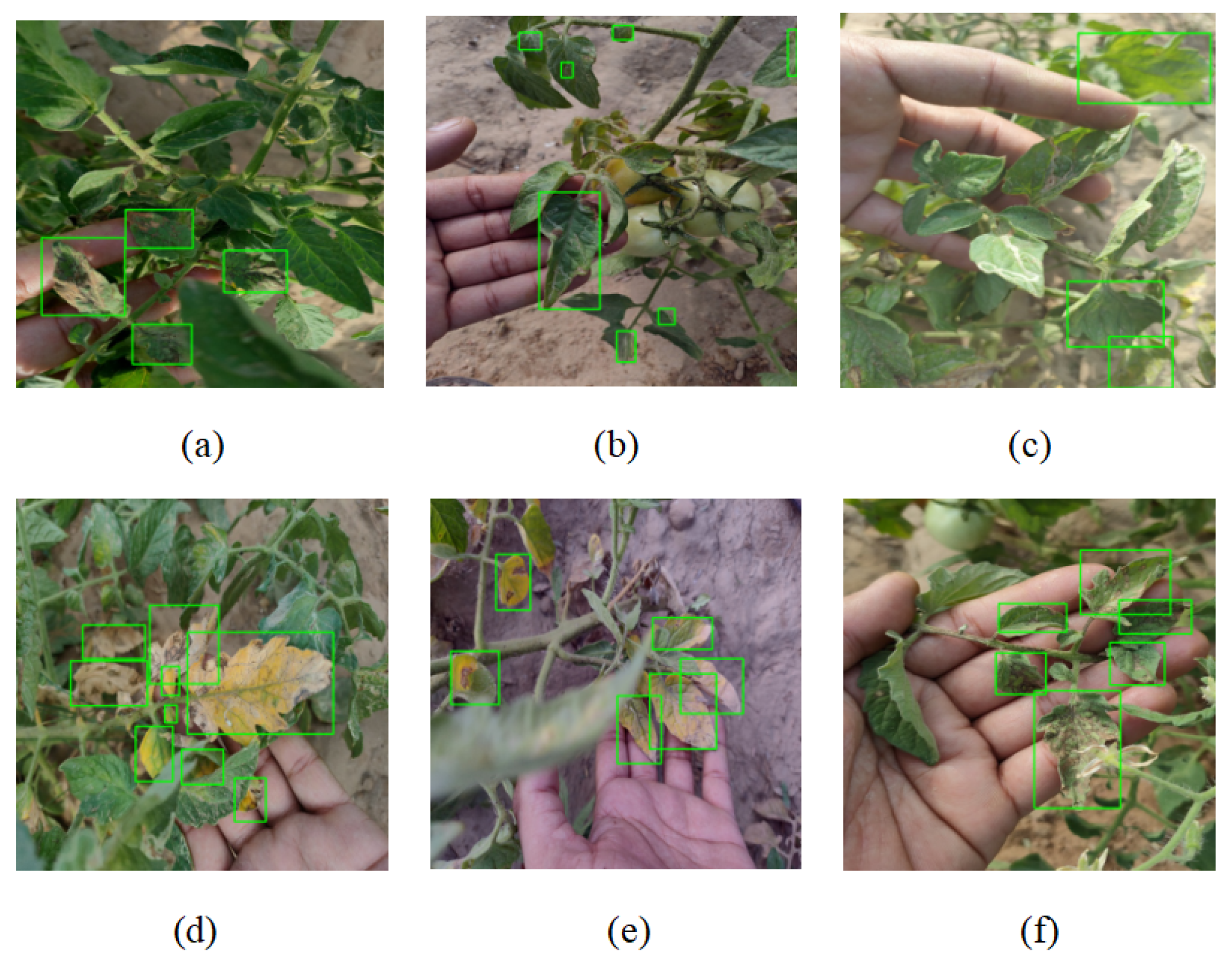
The PlantVillage dataset is currently the most widely used dataset for plant disease detection, containing 54,306 plant leaf images annotated with 38 class labels formatted as “crop–disease” pairs. While it has significantly contributed to plant disease research, its limitations are evident: the majority of images were captured in laboratory or controlled environments, resulting in trained models that underperform in real-world natural settings. To address this, Gehlot et al. [36] curated the Tomato-Village dataset, comprising 14,358 images (640 × 640 × 3 resolution) of tomato plants photographed in natural field environments across Jodhpur and Jaipur, Rajasthan, India. As illustrated in Figure 1, the dataset categorizes six tomato disease states and includes 161,223 labels annotated in YOLO format using LabelImg.

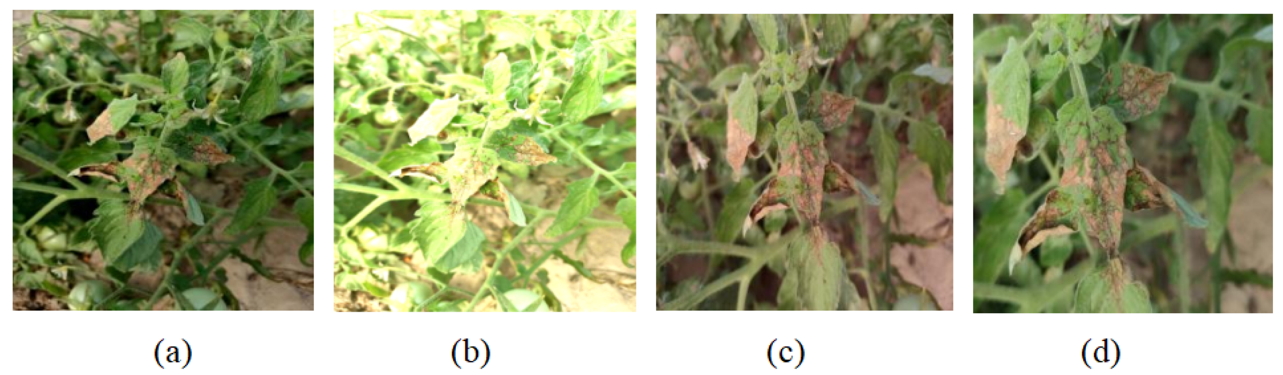
The data augmentation method is shown in Figure 2. Systematic analysis of the Tomato-Village dataset revealed significant data redundancy, where direct utilization of the raw dataset for model training could induce overfitting risks and reduce computational resource efficiency. To mitigate these issues, we implemented a data cleaning strategy by curating 9000 representative images to form the core dataset. Following machine learning best practices, these samples were partitioned into training, validation, and test sets through stratified random sampling at a 7:2:1 ratio to ensure balanced class distributions. Detailed label statistics across subsets are presented in

Table 1. Dataset partition and label distribution.

Dataset	LB	LM	MD	ND	PD	SWV
TRAIN	1912	49,798	7433	802	550	12,853
VAL	226	9139	1340	115	95	4708
TEST	359	7445	1088	83	96	2185

PS: According to the survey, most of the diseases in tomatoes are LM and SWV, so this label accounts for a large proportion in this dataset.

.

3.2. AHN-YOLO

To facilitate comparison of model detection performance in complex environments, we selected the YOLOv series models, trained them under consistent training parameters, and evaluated their performance on the test set. As shown in

Table 2. Performance of YOLOv models on Tomato-Village test set.

Network Model	Precision/%	Recall/%	mAP50/%	Model Size/MB	FPS
YOLOv5-n	56.7	50.5	51.1	4.46	257.9
YOLOv6-n	51.3	40.8	43.7	16.3	283.7
YOLOv8-n	65.5	55.3	59.0	10.7	244.3
YOLOv9-t	66.5	54.7	59.2	8.07	109.3
YOLOv10-n	62.2	53.1	56.9	5.52	169.4
YOLOv11-n	67.3	56.9	62.0	5.25	198.2
YOLOv12-n	65.6	53.4	58.1	5.27	142.5

, YOLOv8 and YOLOv9 demonstrated superior performance in terms of accuracy, but their parameter counts were significantly higher than other models, increasing actual deployment costs. In contrast, YOLOv6 and YOLOv5 achieved the highest FPS and smallest model size, respectively, but their average precision was relatively poor, showing obvious disadvantages in practical applications. Comparatively, YOLOv10, YOLOv11 and YOLOv12 exhibited more balanced performance, among which YOLOv11 performed better—while maintaining higher FPS and fewer parameters, its average precision was approximately 3% higher than other models. Therefore, this paper selected YOLOv11 as the network framework.

As evidenced in Table 2, YOLOv11 demonstrates significant advantages in both real-time detection efficiency and accuracy, which can be attributed to its redesigned backbone network architecture, neck network structure, and the incorporation of the novel C3k2 component. We selected it as our baseline network and further optimized it to enable faster and more accurate detection of diseased plant targets in complex environments.

The current YOLOv11 object detection series comprises five models of varying sizes: YOLOv11n, YOLOv11s, YOLOv11m, YOLOv11l, and YOLOv11x. As the model size increases, the network depth progressively expands to handle more complex environmental detection tasks. To better evaluate the performance improvements of our modified model, we adopted the YOLOv11n framework as our baseline.

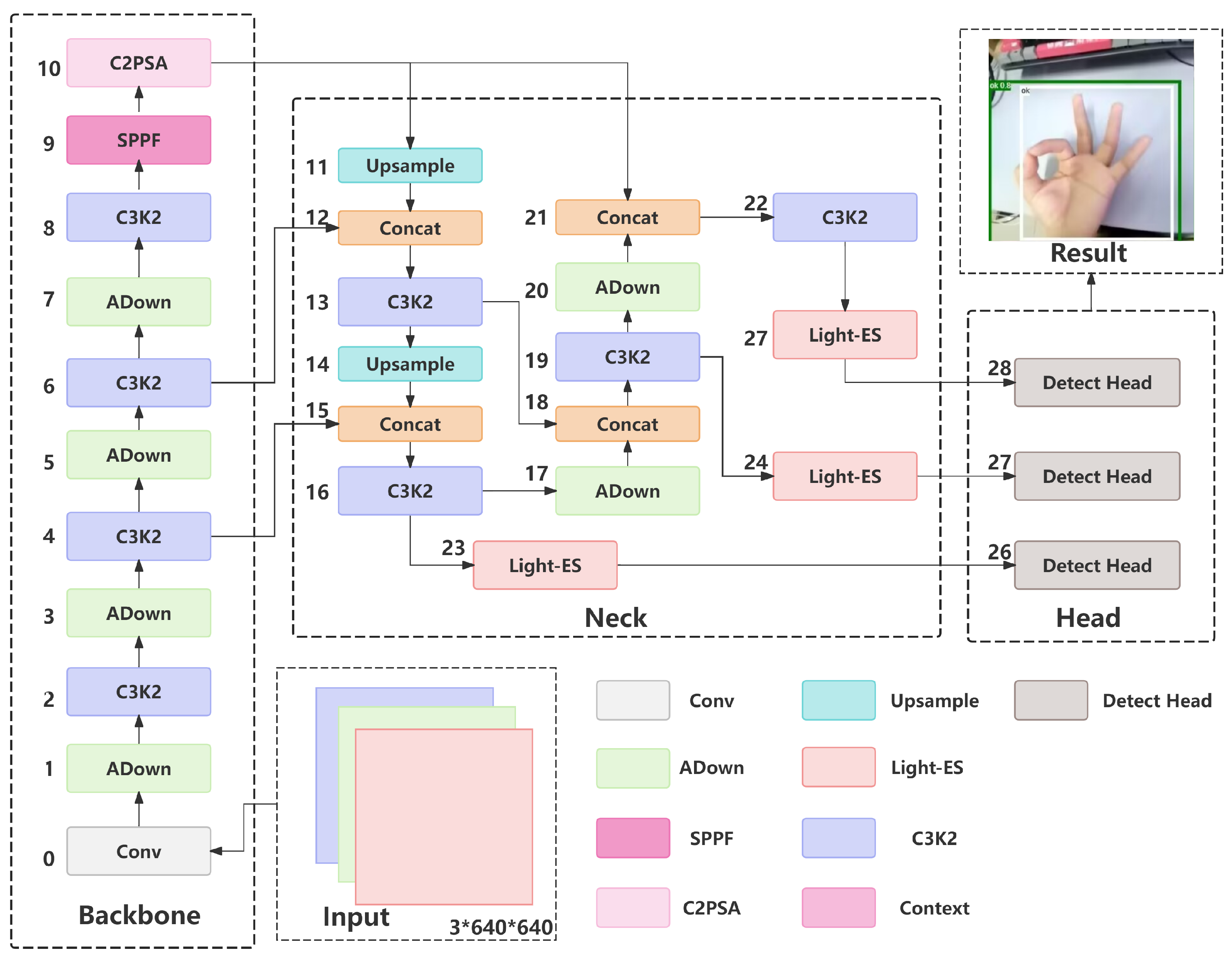
The framework consists of three primary components: the backbone network, neck network, and head network, which respectively perform three core functions: feature extraction, feature fusion, and prediction/classification. Our optimization approach correspondingly focuses on these three components. The overall architecture diagram of our optimized model, AHN-YOLO, is presented in Figure 3.

3.3. Construction of AD-Backbone

The backbone network typically extracts useful features from input images. To extract more subtle features in plant diseases efficiently, we replaced the original Conv layers with ADown modules to optimize the downsampling convolutional components, creating the AD-Backbone. The network processes input images initially sized [640, 640, 3]. It starts with a standard convolutional layer followed by an ADown convolutional layer for downsampling. Both layers use 3 × 3 kernels with a stride of 2 and multiple convolutional kernels to increase the feature map channel depth. A C3K2 convolutional layer then enhances feature extraction. This downsampling pattern of one ADown layer followed by one C3K2 layer repeats three times, generating four feature maps with dimensions [160, 160, 128], [80, 80, 256], [40, 40, 512], and [20, 20, 1024]. We retain the last three feature maps. The final feature map undergoes refinement through SPPF and C2PSA modules sequentially, then concatenates with the preceding two feature maps for input to the neck network.

ADown Module

The recognition of complex images often relies on deep and large-scale convolutional neural networks, which may contain hundreds or even thousands of layers. Their massive parameter counts and computational demands pose significant challenges to computing resources and may cause delays in real-time detection. To address this issue, two primary strategies exist: first, reducing parameters through model compression, and second, optimizing and improving the original network architecture. In the paper “Enhanced YOLOv8 algorithm for leaf disease detection with lightweight GOCR-ELAN module and loss function: WSIoU” [37], Wen et al. replaced the traditional CBS module with the ADown module in the network framework, effectively compressing data volume and parameters while mitigating model overfitting. In the original network architecture, the Conv module aims to reduce feature map resolution to facilitate multi-scale fusion in the neck network. However, this process introduces a substantial number of parameters, increasing the model’s computational burden. To address this, we employ the ADown module to replace the Conv module, maintaining the downsampling functionality while reducing model parameters and computational complexity, further suppressing noise interference in complex environments.

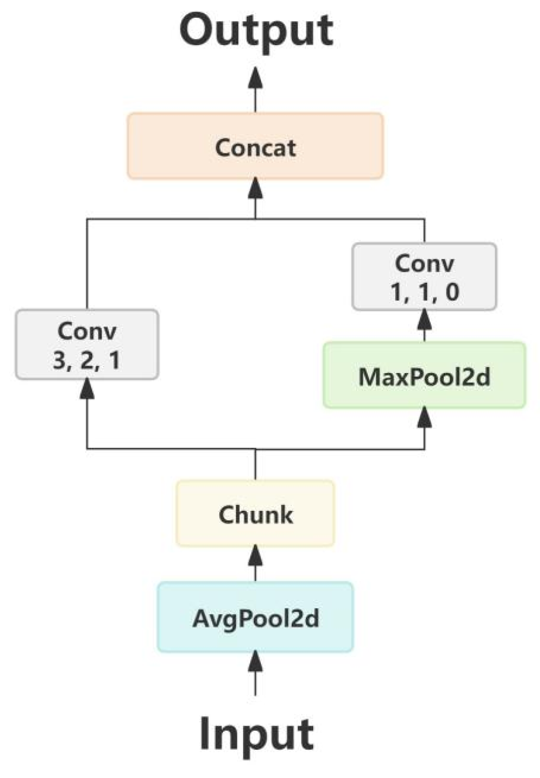
The input feature map first undergoes feature extraction via the C3K2 module, where the feature map has a large width and contains numerous weight parameters. It is then fed into the ADown module, whose implementation steps are illustrated in Figure 4. First, an average pooling layer captures global information from features of different scales, reducing background noise interference. Next, channel splitting halves the input channels, directing them into left and right branches. The left branch combines a 3 × 3 convolutional kernel with average pooling to capture local texture features while reducing resolution. The right branch employs a 1 × 1 convolutional kernel paired with max pooling, focusing on extracting globally salient features.

Assuming the input tensor is $\mathrm{X}\in {\mathbb{R}}^{\mathrm{B}\times \mathrm{C}\times \mathrm{H}\times \mathrm{W}}$, the mathematical formulation of the module’s output is defined in Equations (1) and (2).

$$X{1}_{B,C/2,H,W},X{2}_{B,C/2,H,W}=\mathrm{split}\left(\mathrm{AvgPool}\left(X\right)\right)$$

(1)

$$X_{B,C,H,wW}^{\prime }=\mathrm{Concat}[C_{3\times 3}\left(X{1}_{B,C/2,H,W}\right),C_{1\times 1}\left(\mathrm{MaxPool}\left(X{2}_{B,C/2,H,W}\right)\right)]$$

(2)

The ADown module algorithm reduces the parameter count. For a convolutional kernel size of 3 × 3, the parameter count of traditional downsampling convolution is $P_{conv}=3\times 3\times C_{in}\times C_{out}+3\times 3\times C_{out}\times C_{out}$, while that of the ADown module is $P_{ADown}=3\times 3\times C_{in}\times (C_{out}/2)+1\times 1\times C_{in}\times (C_{out}/2)$. Under identical input and output channel configurations, the ADown module exhibits a significantly lower parameter count and computational load compared to traditional convolution. This indicates that the module enhances training efficiency under constrained training conditions, making it highly suitable for deployment in lightweight models addressing general complex problems.

To elucidate the implementation workflow of the ADown module, we provide its pseudocode below (Algorithm 1), which visually demonstrates the branch processing and feature fusion procedures of input feature maps.

3.4. Design of Light-ES Attention Module

The neck network of the YOLO series employs BiFPN (Bidirectional Feature Pyramid Network), which processes three feature maps of varying dimensions and channel depths for multi-scale feature aggregation to enhance detection accuracy. However, this network relies on fixed-weight cross-scale feature fusion, making it difficult to dynamically adjust the relative importance of features at different levels. This limitation may excessively dilute subtle target details contained in shallow features [38]. To mitigate this drawback, we developed a lightweight hybrid attention mechanism named Light-ES, which is inserted at the terminal output of the neck network as a post-fusion optimization module.

Algorithm 1 ADown Module

Input: Feature map $X\in {\mathbb{R}}^{\mathrm{B}\times \mathrm{C}\times \mathrm{H}\times \mathrm{W}}$

Output: Enhanced feature map $X^{\prime }\in {\mathbb{R}}^{\mathrm{B}\times \mathrm{C}\times \mathrm{H}/2\times \mathrm{W}/2}$

1: Initial Downsampling:   2:    Apply average pooling with kernel size 2 and stride 1:   3:       $X\leftarrow \mathrm{AvgPool}(X,\mathrm{kernel}=2,\mathrm{stride}=1)$     4: Channel Split:   5:    Split X into two equal parts along the channel dimension:   6:       $X1,X2\leftarrow \mathrm{split}(X,\mathrm{axis}=C,\mathrm{ratio}=0.5)$     7: Left Branch (Local Feature Extraction):   8:    Apply $3\times 3$ convolution with stride 2 to $X1$:   9:       $X1\leftarrow \mathrm{Conv}3\times 3(X1,\mathrm{stride}=2,\mathrm{padding}=1)$   10: Right Branch (Global Feature Extraction): 11:    Apply max pooling with kernel size 3 and stride 2 to $X2$: 12:       $X2\leftarrow \mathrm{MaxPool}(X2,\mathrm{kernel}=3,\mathrm{stride}=2,\mathrm{padding}=1)$ 13:    Apply $1\times 1$ convolution to $X2$: 14:       $X2\leftarrow \mathrm{Conv}1\times 1(X2,\mathrm{stride}=1,\mathrm{padding}=0)$   15: Feature Fusion: 16:    Concatenate outputs from both branches: 17:       $X^{\prime }\leftarrow \mathrm{Concat}(X1,X2,\mathrm{axis}=C)$ 18: Return $X^{\prime }$

The Light-ES module consists of parallel SimAM and ECA components that perform weighted refinement on multi-scale input feature maps. This design strengthens the model’s localization and classification capabilities while serving as a preprocessing step for subsequent detection heads, ultimately improving detection performance in complex scenarios. By adaptively enhancing feature representation, Light-ES effectively compensates for BiFPN’s static fusion mechanism while maintaining computational efficiency.

3.4.1. SimAM Model

The SimAM (Similarity-Aware Activation Module) [29] represents an innovative attention mechanism grounded in the local self-similarity of feature maps and characterized by its parameter-free design. Specifically, it dynamically adjusts pixel weights based on the similarity between pixels within the feature map, thereby amplifying task-critical features while suppressing irrelevant ones. This property enables SimAM to efficiently capture key information when processing small-scale features, avoiding overfitting or information loss caused by excessive parameters and significantly enhancing model performance in fine-grained feature extraction tasks.

The implementation steps of SimAM are as follows: Assume an input tensor with batch size B,  C channels, and spatial dimensions H × W. SimAM first computes the mean and variance across the spatial dimensions (H × W) for each sample and channel within the input tensor. These statistical measures reflect the distribution of activation values at different spatial positions within the same channel. For the c-th channel of the b-th sample, the formulas for mean and variance are provided in Equations (3) and (4).

$${\mu }_{b,c}={\displaystyle \frac{1}{H\times W}}\sum _{h=1}^H\sum _{w=1}^W{x}_{b,c,h,w}$$

(3)

$${\sigma }_{b,c}^2={\displaystyle \frac{1}{H\times W}}\sum _{h=1}^H\sum _{w=1}^W{(x_{b,c,h,w}-{\mu }_{b,c})}^2$$

(4)

To effectively implement attention mechanisms, it is essential to evaluate the importance of each neuron. In neuroscience, neurons exhibiting spatial inhibition effects should be assigned higher importance, and the simplest method to identify such neurons is to measure the linear separability between a target neuron and others. Consequently, the previously mentioned variance and mean can be utilized to formulate an energy computation equation (Equation (5)) that quantifies the relative saliency of a pixel within its corresponding sample and channel positions.

$$E_{b,c,h,w}={\displaystyle \frac{{(x_{b,c,h,w}-{\mu }_{b,c})}^2}{4\times ({\sigma }_{b,c}^2+\lambda )}}+1/2$$

(5)

The operations of multiplying by 1/4 and adding 1/2 are designed to normalize the energy values into the effective working range of the Sigmoid function, thereby mitigating issues such as gradient vanishing or exploding gradients. Subsequently, the energy values are mapped to the [0, 1] interval via the Sigmoid activation function (Equation (6)), generating attention weights. These weights are then element-wise multiplied with the original input tensor (Equation (7)) to produce a weighted feature map.

$$Sigmoid\left(x\right)={\displaystyle \frac{1}{1+e^{-x}}}$$

(6)

$$X_{b,c,h,w}^{\prime }=X_{b,c,h,w}\times Sigmoid\left(E_{b,c,h,w}\right)$$

(7)

Through this process, the SimAM module assigns a unique weight to each neuron, significantly enhancing the model’s ability to focus on complex, densely distributed features.

3.4.2. ECA Model

ECA (Efficient Channel Attention) [30] is a channel attention mechanism designed to enhance the ability of convolutional neural networks (CNNs) to assess the importance of individual channels. This mechanism extends the SE (Squeeze-and-Excitation) attention framework. While the SE module computes channel attention via fully connected (FC) layers—a method prone to computational redundancy—the ECA module employs a simplified one-dimensional convolution operation, significantly improving computational efficiency.

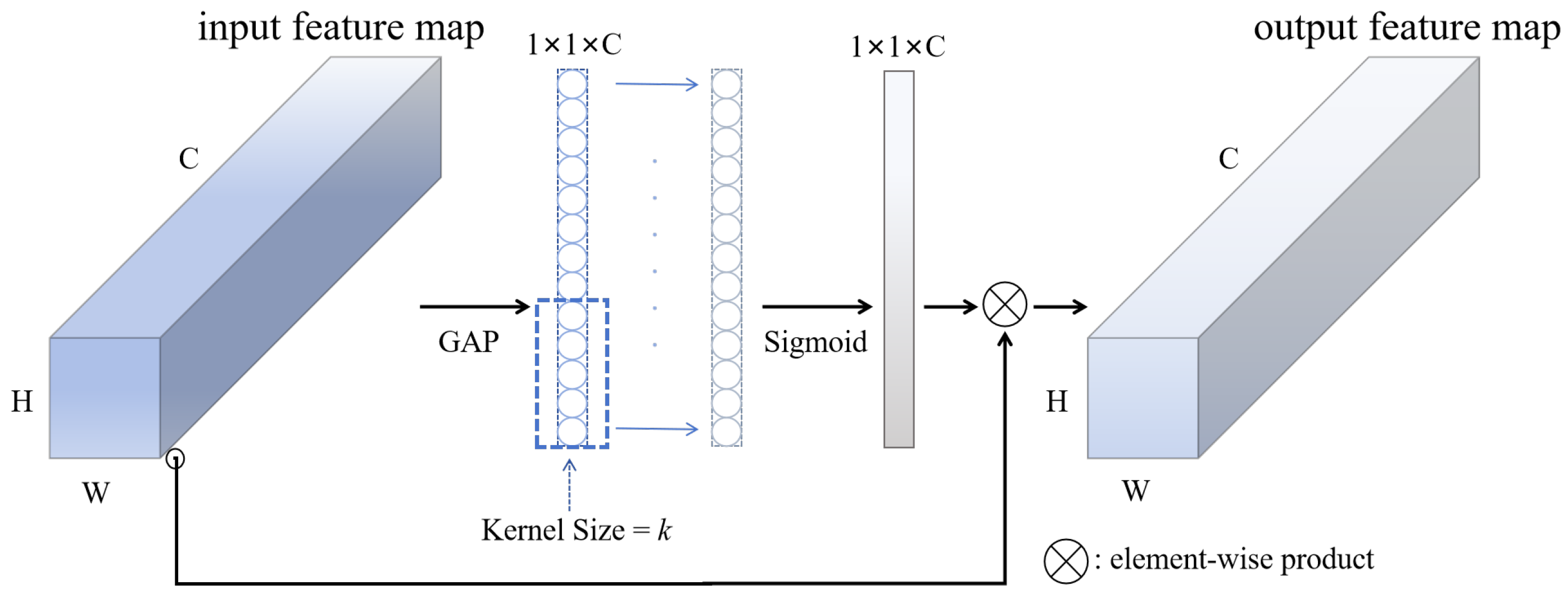
The implementation steps of ECA are shown in Figure 5: The ECA module first applies Global Average Pooling (GAP) to the input feature map $\mathrm{X}\in {\mathbb{R}}^{\mathrm{B}\times \mathrm{C}\times \mathrm{H}\times \mathrm{W}}$, aggregating global spatial information into a one-dimensional vector $\mathrm{X}\in {\mathbb{R}}^{\mathrm{B}\times \mathrm{C}\times 1\times 1}$. Next, the optimal receptive field length k for the one-dimensional convolutional kernel is determined using a theoretically derived formula (Equation (8)).

$$k={\displaystyle \frac{\log \left(2\right)}{\log \left(\sqrt{(C/\gamma )+b}\right)}}$$

(8)

where $\mathrm{C}$ denotes the number of input channels, and $\gamma$, $\mathrm{b}$ are hyper-parameters set to 2 and 1 by default. This formula ensures effective capture of inter-channel dependencies. The output is then normalized to the [0, 1] interval via a Sigmoid activation function, generating channel-wise attention weights. Finally, these weights are multiplied channel-wise with the original feature map to accomplish feature recalibration.

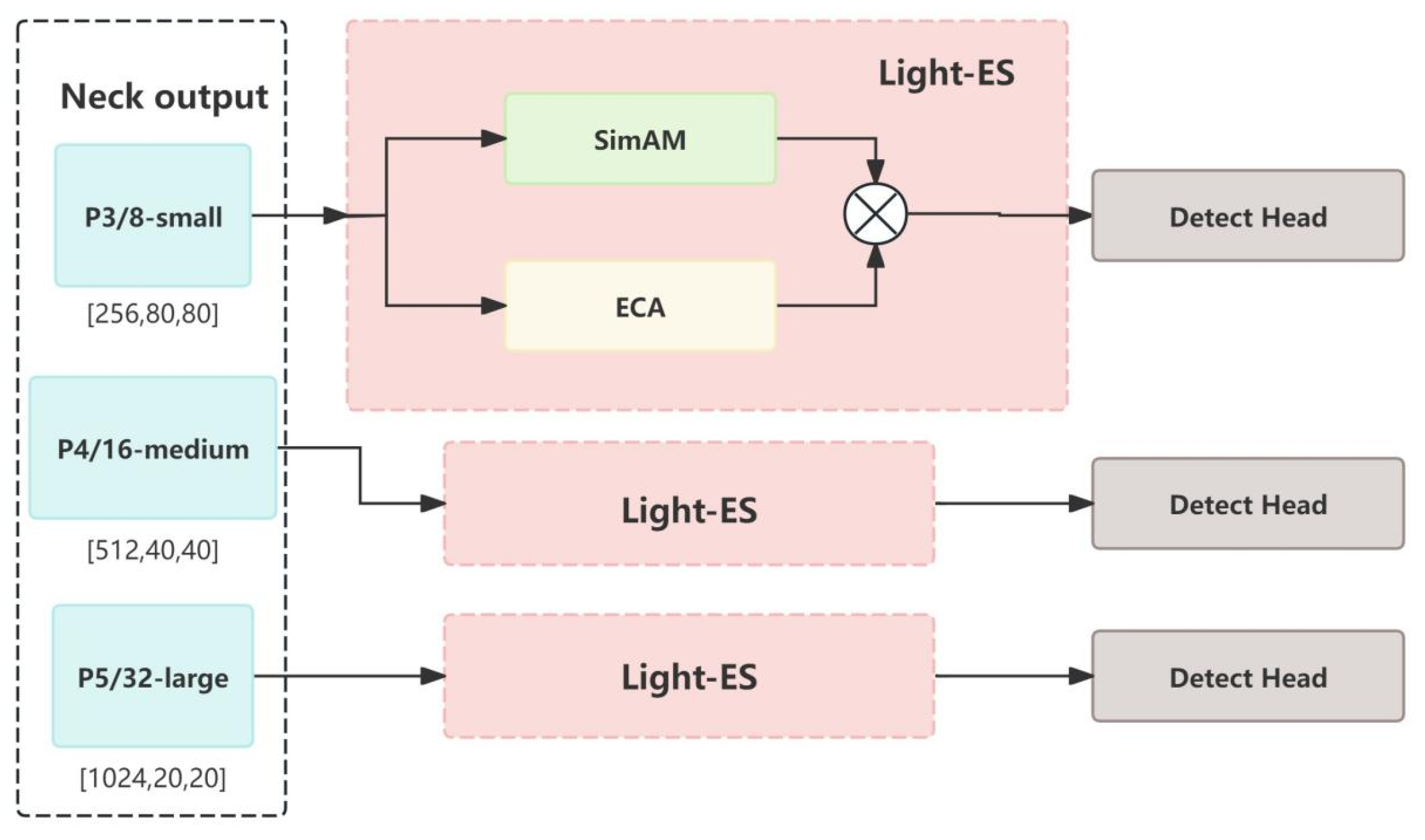
3.4.3. Light-ES Model

To enable the model to effectively detect dense, small-sized pathological features in complex environments, capturing global information helps the model better recognize target characteristics amidst various interfering factors and complex backgrounds, thereby reducing false positives and missed detections. Meanwhile, in datasets with dense feature distributions, subtle differences in local features may be critical for target identification, making detailed local feature extraction equally essential.

To address these requirements, we designed a hybrid attention mechanism for global–local information processing, incorporating both ECA (Efficient Channel Attention) and SimAM (Similarity-based Attention Module) modules. The ECA module employs 1D convolution to capture inter-channel dependencies, enhancing the model’s perception of global information. The SimAM module dynamically adjusts pixel-wise weights by calculating similarity between each pixel and its neighbors, thereby improving the model’s focus on local details. By processing these two modules in parallel and fusing their outputs through weighted integration, the model simultaneously attends to both global and local features, enabling more effective handling of dense small targets. For the tomato dataset containing dense small features, the ECA module improves the model’s sensitivity to subtle features by modeling channel-wise relationships, while the SimAM module enhances localized attention through adaptive pixel weighting. This dual focus on global and local information significantly boosts the model’s capability to extract small features. Both ECA and SimAM are lightweight attention mechanisms with relatively low algorithmic complexity, avoiding substantial computational overhead while maintaining performance—theoretically improving computational efficiency and real-time capability.

As illustrated in Figure 6, we positioned this mechanism ahead of the three detection heads. The input consists of three feature maps with varying dimensions and channel depths, allowing the module to maximally extract discriminative features across all scales and thereby elevate overall detection performance.

The implementation steps of this hybrid attention mechanism are as follows: Input feature maps are fed in parallel into the ECA and SimAM modules. After computation by these modules, the resulting parameters are fused through weighted summation, as shown in Equation (9).

$$X_{HES}={\omega }_1\times X_{SimAM}+{\omega }_2\times X_{ECA}$$

(9)

The weights ${\omega }_1$ and ${\omega }_2$ are dynamically adjusted during model training via forward propagation algorithms, completing the construction of the hybrid attention mechanism.

To elucidate the implementation workflow of the light-ES module, we provide its pseudocode below (Algorithm 2), which visually demonstrates the branch processing and feature fusion procedures of input feature maps.

Algorithm 2 Light-ES Hybrid Attention Module

Input: Feature map $X\in {\mathbb{R}}^{\mathrm{B}\times \mathrm{C}\times \mathrm{H}\times \mathrm{W}}$

Output: Enhanced feature map $X^{\prime }\in {\mathbb{R}}^{\mathrm{B}\times \mathrm{C}\times \mathrm{H}\times \mathrm{W}}$

1: Local Attention (SimAM):   2:    Compute mean $\mu$ of X over spatial dimensions:   3:       $\mu \leftarrow \mathrm{Mean}(X,\dim =[H,W],\mathrm{keepdim}=\mathrm{True})$   4:    Compute variance-like energy E:   5:       $E\leftarrow {\displaystyle \frac{{(X-\mu )}^2}{4\times (\mathrm{Mean}\left({(X-\mu )}^2\right)+ϵ)}}+0.5$   6:    Apply Sigmoid to energy E:   7:       $S_{\mathrm{local}}\leftarrow \mathrm{Sigmoid}\left(E\right)$   8:    Generate local-attention enhanced feature:   9:       $X_{\mathrm{local}}\leftarrow X\odot S_{\mathrm{local}}$ 10: Global Attention (ECA): 11:    Compute global average pooling: 12:       $G\leftarrow \mathrm{AvgPool}\left(X\right)$ 13:    Apply 1D convolution to G (kernel size k): 14:       $G\leftarrow \mathrm{Conv}1\mathrm{D}(G,\mathrm{kernel}=k)$ 15:    Apply Sigmoid to generate channel weights: 16:       $S_{\mathrm{global}}\leftarrow \mathrm{Sigmoid}\left(G\right)$ 17:    Generate global-attention enhanced feature: 18:       $X_{\mathrm{global}}\leftarrow X\odot S_{\mathrm{global}}$ 19: Hybrid Fusion: 20:    Assign learnable weights ${\omega }_1$, ${\omega }_2$ to local and global features: 21:       $X^{\prime }\leftarrow {\omega }_1·X_{\mathrm{local}}+{\omega }_2·X_{\mathrm{global}}$ 22: Return $X^{\prime }$

3.5. Head Network Optimization

Compared to previous YOLO versions, YOLOv11 introduces two additional DWConv (Depthwise Separable Convolution) layers in its classification detection head to reduce computational overhead. Furthermore, it incorporates the EIoU (Extended IoU) loss function, which considers the overlap area, aspect ratio, and center offset between predicted and ground-truth bounding boxes, thereby improving localization accuracy. Given its superior performance, we retained YOLOv11’s detection head structure for final image processing. In this architecture, the bounding box regression loss combines CIoU and DFL (Distribution Focal Loss), which quantifies the discrepancy between predicted and ground truth boxes, playing a critical role in model parameter optimization. While CIoU demonstrates excellent performance for medium- and large-sized targets, it shows limitations in small object detection [39]. To address this, we integrated NWD (Normalized Wasserstein Distance) with CIoU to create the NWD-CIoU loss function, enabling more robust handling of targets across varying scales.

NWD-CIoU Loss Function

In complex natural scenarios, dense small-target detection faces dual challenges of geometric feature ambiguity and environmental noise interference. Small targets typically occupy only a few to dozens of pixels in an image, and their bounding box regression is susceptible to positional sensitivity, gradient imbalance, and shape constraint limitations, resulting in poor localization accuracy. To enhance the model’s precision and efficiency for small-target detection, we introduce the Normalized Wasserstein Distance (NWD) algorithm—a novel approach leveraging Wasserstein distance for small-target detection—and integrate it with CIoU to optimize the existing loss function. First, the NWD-CIoU loss function retains CIoU’s geometric alignment terms, enforcing spatial consistency between predicted and ground truth bounding boxes through Equation (10).

$$CIoU=IoU-{\displaystyle \frac{{\rho }^2(b,b^{gt})}{c^2}}-\alpha v$$

(10)

Here, $\rho$ represents the Euclidean distance between centers, c denotes the diagonal length of the minimum enclosing rectangle, v signifies the aspect ratio of the anchor box, $\alpha v$ corresponds to the aspect ratio penalty term, and w and h are the width and height of the anchor box, respectively. This module ensures that the model’s localization accuracy for medium and large targets remains uncompromised.

For small-target detection, most bounding boxes are not strictly rectangular. A bounding box $R=(c_x,c_y,w,h)$ inevitably contains background pixels. To better prioritize and enhance pixel-level relevance for small objects, a 2D Gaussian distribution is introduced to model the bounding box, where the central pixels exhibit the highest weights, decaying gradually toward the periphery. The formula for this 2D Gaussian distribution is defined in Equation (11).

$$f\left(X\right)={\displaystyle \frac{\exp \left[-\frac{1}{2}{(X-\mu )}^T{\Sigma }^{-1}(X-\mu )\right]}{{\left(2\pi \right)}^{d/2}{|\Sigma |}^{1/2}}}$$

(11)

where $f\left(X\right)$ denotes the computed pixel weight, X represents the coordinates of a pixel $(x,y)$, $\mu =\left[\begin{array}{c}{c}_x\\ c_y\end{array}\right]$ is the mean vector, and $\Sigma =\left[\begin{array}{cc}{w}^2/4& 0\\ 0& h^2/4\end{array}\right]$ is the covariance matrix.

Subsequently, the Wasserstein distance from optimal transport theory is employed to measure the distance between the predicted bounding box $R_g=(c_{xg},c_{yg},w_g,h_g)$ and the ground-truth bounding box $R_t=(c_{xt},c_{yt},w_t,h_t)$, which are modeled as Gaussian distributions $N_g$ and $N_t$, respectively; the Wasserstein distance between these two bounding boxes can be further simplified to Equation (12).

$$W_2^2(N_g,N_t)={∥\left({\left[\begin{array}{c}{c}_{xg},c_{yg},{\displaystyle \frac{w_g}{2}},{\displaystyle \frac{h_g}{2}}\end{array}\right]}^T,{\left[\begin{array}{c}{c}_{xt},c_{yt},{\displaystyle \frac{w_t}{2}},{\displaystyle \frac{h_t}{2}}\end{array}\right]}^T\right)∥}_2^2$$

(12)

Here, ${\parallel ·\parallel }_F$ denotes the Frobenius norm. At this stage, $W_2^2(N_1,N_2)$ remains a distance metric and cannot directly serve as a similarity measure bounded within [0, 1]. To address this, we normalize $W_2^2(N_1,N_2)$ via an exponential transformation to derive the Normalized Wasserstein Distance (NWD), as defined in Equations (13) and (14).

$$NWD(N_g,N_t)=\exp \left(-{\displaystyle \frac{\sqrt{W_2^2(N_g,N_t)}}{C}}\right)$$

(13)

$$NWD\_IoU=1-NWD(N_g,N_t)$$

(14)

where C is the normalization coefficient used to scale the Wasserstein distance, ensuring that the NWD value is bounded within a reasonable range. The resulting NWD-IoU loss increases as the distance $W_2^2(N_1,N_2)$ between predicted and ground-truth bounding boxes grows, and vice versa. This loss function exhibits scale invariance to minor positional deviations in small targets, preventing pixel-level errors from being overshadowed.

Finally, a tunable ratio $\gamma$ is introduced to balance the contributions of CIoU and NWD-IoU, optimizing the module’s performance for both small and medium to large targets in the dataset. The formulation is given in Equation (15).

$$L_{NWD-CIoU}=\gamma \times CIoU+(1-\gamma )\times NWD\_IoU$$

(15)

4. Experimental Results and Analysis

4.1. Experimental Environment

The hardware and software environment of our experimental part are shown in

Table 3. Hardware and software environment overview.

Category	Details
Environment Category	Intel Core i7-12700H CPU
	Micron_3400_MTFDKBA512TFH 477GB SSD
	NVIDIA GeForce RTX 3060 Laptop GPU
	16GB Memory
Software Environment	Pycharm 2024.1.2
	Python 3.8
	Torch 2.4.1
	CUDA Toolkit 11.8

.

To ensure the rigor of the experiments, we initially conducted trials using the YOLOv11 model. However, we observed that when the training epochs exceeded 120, the performance metrics exhibited a diminishing growth trend, indicating overfitting. Consequently, we set the training epoch to 100, a value that was consistently applied in both ablation and comparative experiments. The training parameters utilized in the experiment are detailed in

Table 4. Model training hyper-parameters.

Model Hyper-Parameter	Method/Value
Batch size	16
Optimizer	SGD
Weight_decay	0.0005
Training epoch	100
Momentum	0.937
Device	cuda
Box_weight	7.5
Cls_weight	0.5
Dfl_weight	1.5

.

4.2. Evaluation Metrics

Accuracy measures the proportion of correctly identified objects among all detected objects. In object detection, a high accuracy indicates that the model effectively reduces false positives. The formula is given in Equation (16).

$$Precision={\displaystyle \frac{TP}{TP+FP}}$$

(16)

Recall reflects the model’s ability to capture all actual objects. A high recall suggests that the model can detect most of the real targets, minimizing missed detections. The corresponding formula is provided in Equation (17).

$$Recall={\displaystyle \frac{TP}{TP+FN}}$$

(17)

where TP (true positive) refers to correctly detected objects, FP (false positive) denotes incorrectly detected objects such as background misclassified as targets, and FN (false negative) represents missed detections. Mean average precision (mAP) is the most commonly used comprehensive metric in object detection. It considers the model’s detection precision across different categories. By averaging the average precision (AP) of each category, mAP provides a holistic evaluation of the model’s detection capability. The AP formula is given in Equation (18), while mAP is computed based on the average AP across all categories, as shown in Equation (18).

$$AP={\int }_0^{1}p\left(r\right)dr$$

(18)

Let represent precision on the precision–recall (P-R) curve. The mAP value is obtained by averaging the AP values across all categories, following Equation (19).

$$mAP={\displaystyle \frac{1}{N}}\sum _{i=1}^{N}A{P}_i$$

(19)

where N is the total number of categories, and $A{P}_i$ denotes the average precision for the i-th category. In practice, mAP50 is commonly used for evaluation, where 50 signifies an Intersection over Union (IoU) threshold of 50%. IoU measures the overlap between the predicted bounding box and the ground-truth bounding box, as defined in Equation (20).

$$IoU={\displaystyle \frac{\mathrm{Area}\mathrm{of}\mathrm{Overlap}}{\mathrm{Area}\mathrm{of}\mathrm{Union}}}$$

(20)

Frames Per Second (FPS) is used to assess the real-time performance of the model, indicating the number of image frames processed per second. A higher FPS not only signifies faster detection speed but also ensures system responsiveness in real-world deployment, enabling timely capture of dynamic changes. The FPS computation is given in Equation (21).

$$FPS={\displaystyle \frac{\mathrm{Total}\mathrm{Frames}\mathrm{Processed}}{\mathrm{Total}\mathrm{Time}}}$$

(21)

4.3. Experimental Results

4.3.1. Comparative Experiments on Lightweight Attention Mechanisms

To validate the effectiveness of our proposed lightweight hybrid attention mechanism Light-ES in complex detection scenarios, we conducted systematic comparative experiments under identical training parameter settings, benchmarking it against mainstream lightweight attention modules including SE (Squeeze-and-Excitation), EMA (Efficient Multi-scale Attention), SimAM, ECA, and CGA (Cascaded Group Attention). Detailed experimental results are presented in

Table 5. Comparison of lightweight attention mechanisms on test set.

Network Model	Precision/%	Recall/%	mAP50/%	Parameters/M	FPS
YOLOv11	67.3	56.9	62.0	2.6	200.3
YOLOv11+CGA	54.0	51.0	51.3	2.5	132.2
YOLOv11+EMA	57.8	51.4	53.3	2.4	194.3
YOLOv11+iRMB	63.2	53.0	57.2	2.8	193.5
YOLOv11+SE	68.1	56.7	61.1	2.6	201.7
YOLOv11+SimAM	68.3	58.6	62.5	2.6	183.8
YOLOv11+ES	69.4	59.0	64.1	2.6	193.6

, with heatmap visualizations shown in Figure 7.

Traditional attention modules exhibit three core contradictions in complex agricultural scenarios. The CGA module, despite its cascaded global attention design attempting to balance efficiency and precision, demonstrates degraded FPS and mAP50 metrics. Heatmap analysis reveals accurate plant localization but insufficient lesion region capture, exposing imbalance between global modeling and local feature extraction. The EMA module reduces parameters to 2.4 M through multi-scale feature compression, effectively suppressing background noise at the cost of small-target feature loss, confirming the precision bottleneck of single-scale compression in dense detection scenarios. Simplified mechanisms like SE and SimAM improve computational efficiency but achieve significantly lower mAP50 and recall than baseline models. Heatmaps indicate amplified background noise and attention region omission, highlighting the precision limitations of over-reliance on single-dimensional weight allocation in complex environments.

In contrast, Light-ES achieves breakthrough improvements through its local-global dynamic coupling mechanism. Under a 2.6 M parameter constraint, the YOLOv-ES model equipped with this mechanism achieves 69.4% precision, 59.0% recall, and 64.1% mAP50, while maintaining comparable frame rates (193.6 FPS vs. baseline 198.2 FPS). Heatmap visualizations demonstrate Light-ES’s dual capability: preserving shallow lesion details while suppressing background interference through global context modeling, with background denoising effectiveness surpassing all comparative modules. The experimental results demonstrate that Light-ES successfully addresses three critical limitations of conventional modules: substantial reduction in background interference sensitivity, maintenance of superior small-target feature retention rates, and elimination of architectural rigidity through adaptive attention allocation. This tripartite optimization enables optimal balance across parameter count, computational efficiency, and detection accuracy under multidimensional constraints.

In conclusion, Light-ES provides an ideal solution for agricultural edge computing scenarios, satisfying both low-cost deployment requirements and precision demands in complex environments. Its superior performance in multi-scale, dense crop disease monitoring tasks establishes a new benchmark for practical agricultural vision systems.

4.3.2. Comparative Experiments on Improved Loss Functions

In Section 4.3.1, we present the proposed innovative NWD-CIoU loss function, which strategically combines the advantages of two distinct loss algorithms through weighted fusion. To determine the optimal fusion ratio for subsequent comparative analysis, we conducted controlled experiments with varying weight configurations while maintaining identical training parameters on our modified model architecture. The experimental results are detailed in

Table 6. Loss function fusion weight comparison.

Fusion Ratio	Precision/%	Recall/%	mAP50/%
0	76.1	62.0	70.4
0.1	77.0	63.4	70.0
0.2	74.5	62.7	69.5
0.3	73.3	62.9	69.2
0.4	76.8	64.4	71.2
0.5	68.9	60.5	64.7
0.6	72.9	60.0	67.1
0.7	72.5	62.5	68.2
0.8	67.1	61.6	65.0
0.9	70.5	61.2	65.5
1.0	70.9	61.2	66.1

.

As evidenced by the data in the table, when the fusion ratio is set to 0.4 (with CIoU accounting for 40% and NWD for 60% of the loss function), the model achieves optimal performance across all evaluation metrics, including mean average precision. Consequently, we selected 0.4 as the fusion ratio for the NWD-CIoU loss function.

To comprehensively evaluate the compatibility of the NWD-CIoU loss function with our innovative model and its superior performance in specific detection scenarios, we conducted comparative experiments with multiple loss functions, including CIoU (balanced across detection metrics), SIoU (excelling in slender object detection through angular penalty terms and scale sensitivity mechanisms), EIoU (resolving high-similarity target confusion via center-distance constraints and minimum bounding box regularization), and FocusLoss (enhancing small-target detection through spatial attention modulation). Notably, we developed three novel composite loss functions—Focaler-CIoU, Focaler-SIoU, and Focaler-EIoU—by strategically fusing FocusLoss’s attention mechanism with CIoU, SIoU, and EIoU, respectively, through a 7:3 weighted integration strategy (This hybrid leverages FocusLoss’s spatial attention to amplify small-target features while baseline losses enforce geometric constraints, jointly boosting small-target sensitivity and localization accuracy. Crucially, it replaces fixed-ratio fusion with dynamic weight allocation—innovating beyond traditional focal loss). The comparative experimental results, systematically presented in Figure 8 and Figure 9, reveal critical performance variations across these loss configurations under complex agricultural detection conditions.

Table 7. Final training metrics for loss function variants.

Fusion Ratio	Bounding Box Loss	Total Loss	mAP50/%
CIoU	3.19	15.61	61.4
EIoU	3.02	15.17	59.2
SIoU	3.17	15.55	60.7
FocusLoss	2.90	13.37	58.1
Focaler-CIoU	2.86	13.27	61.0
Focaler-SIoU	2.83	13.18	60.4
Focaler-EIoU	2.74	12.92	57.7
NWD-CIoU	2.45	9.89	64.3

presents the model performance metrics of each comparative loss function at the 100th training epoch. By combining the training process metrics from Figure 8 and Figure 9, we observe that compared to the original CIoU in the baseline model, SIoU, FocusLoss and EIoU—which are suitable for fine-grained object detection—demonstrate inferior performance in terms of final mAP. Specifically, although EIoU reduced the localization loss and total loss by 58.5% and 57.4%, respectively (exceeding CIoU’s reductions of 56.6% and 57.1%), its mAP decreased by 1.2%. SIoU achieved 56.3% and 56.6% reduction in localization loss and total loss, respectively, showing slightly inferior efficiency to EIoU and CIoU in terms of loss function performance, but achieved better mAP than EIoU. The suboptimal performance of EIoU and SIoU stems from their fundamental reliance on bounding box geometric IoU for loss construction, where gradient computation exhibits excessive dependence on absolute coordinate positions. Minor positional deviations of small targets—often spanning merely a few pixels—induce drastic IoU fluctuations, consequently degrading mean average precision. In contrast, the NWD-based approach resolves this gradient oscillation challenge through Gaussian distribution modeling of bounding boxes, which measures feature similarity via probabilistic distribution alignment rather than rigid coordinate matching. This statistical paradigm demonstrates superior stability in handling small-target localization uncertainties inherent to agricultural detection scenarios. Meanwhile, FocusLoss reduced localization loss and total loss by 59.5% and 61.8%, respectively, representing the highest efficiency among all individual loss functions under comparison, yet it performed worst in terms of mAP. Given FocusLoss’s advantage in loss function efficiency, we combined it with better-performing loss functions (CIoU, EIoU and SIoU) using a fusion weight of 0.7. The results show that while FocusLoss can effectively improve the convergence efficiency of the loss function, its negative impact on mAP remains significant.

The NWD-CIoU achieves a mAP of 64.3%, representing a 2.9% improvement over the original CIoU. While its total loss reduction (61.6%) marginally trails FocusLoss, the distribution-geometry dual-driven mechanism enables optimal balance between loss convergence efficiency and detection precision. Notably, within this dataset dominated by small detection targets that pose significant challenges, these results validate NWD-CIoU’s superiority in small-object scenarios: by replacing absolute coordinate dependency with probabilistic distribution modeling, it fundamentally overcomes the hypersensitivity inherent in IoU-based functions.

4.3.3. Ablation Experiments

Table 8. AHN-YOLO ablation study results.

Method	AD	ES	NC	Precision (%)	Recall (%)	mAP50 (%)	Parameters (M)	FPS
YOLOv11-n (A)				67.3	56.9	62.0	2.6	198.2
A-YOLO (B)	✓			68.1	62.4	65.7	2.1	176.2
H-YOLO (C)		✓		69.4	59.0	64.1	2.6	183.5
N-YOLO (D)			✓	69.2	58.7	64.3	2.6	205.4
AH-YOLO (E)	✓	✓		70.3	60.9	65.9	2.1	161.5
AN-YOLO (F)	✓		✓	70.1	60.4	65.9	2.1	187.5
HN-YOLO (G)		✓	✓	73.4	58.5	66.4	2.6	174.6
AHN-YOLO (H)	✓	✓	✓	76.8	64.4	71.2	2.1	165.5

Attention: The meaning of “✓” is that this module exists in the model.

and

Table 9. Cross-validation experimental results of AHN-YOLO.

Method	Fold 1 (%)	Fold 2 (%)	Fold 3 (%)	Fold 4 (%)	Fold 5 (%)	Mean ± Std	vs. Baseline (t-test)
YOLOv11-n (A)	55.9	63.3	62.5	61.5	62.5	61.34 ± 2.86	-
A-YOLO (B)	59.2	63.2	65.0	65.1	64.6	63.42 ± 2.14	$\uparrow 2.08(p=0.112)$
H-YOLO (C)	57.8	64.0	64.5	64.2	64.7	63.04 ± 2.47	$\uparrow 1.70(p=0.160)$
N-YOLO (D)	60.1	66.3	66.4	65.5	65.9	64.84 ± 2.31	$\uparrow 3.50(p=0.007)$
AH-YOLO (E)	60.2	64.5	66.3	65.3	64.9	64.24 ± 1.98	$\uparrow 2.90(p=0.016)$
AN-YOLO (F)	62.2	67.3	68.0	66.7	67.5	66.34 ± 2.06	$\uparrow 3.50(p<0.001)$
HN-YOLO (G)	61.9	67.8	68.5	65.9	68.7	66.56 ± 2.60	$\uparrow 5.22(p=0.003)$
AHN-YOLO (H)	63.6	70.2	69.2	67.6	69.6	68.04 ± 2.54	$\uparrow 6.70(p<0.001)$

Attention: The meaning of “↑” is that the model improved on the baseline mAP, and the following number is the percentage improvement.

present the ablation study results of the proposed modules—ADown (abbreviated as AD), Light-ES (ES), and NWD-CIoU (NC)—on the YOLOv11-n framework under unified dataset training and cross-validation ablation experiments, respectively. All models strictly adhered to the predefined training parameters described earlier, undergoing 100 training epochs before evaluation on the test set. For clarity in presentation and subsequent comparative analysis, the models are systematically labeled A through H in the tables.

In terms of computational speed (FPS), models D, F and G incorporating NC demonstrated relative speed improvements compared to their NC-free counterparts A and E. Although model H showed decreased FPS, its frame rate still met the requirements for practical lightweight application deployment. Comparing model A with B, we observed that while reducing parameters (from 2.6 M to 2.1 M), B simultaneously improved detection accuracy (from 67.3% to 68.1%, 62.0% to 65.7%). This indicates that when replacing the downsampling module, the AD module can effectively reduce computational load and parameters while preserving feature information and reducing background noise through average and max pooling, thereby enhancing feature extraction capability.

The comparison between A and C revealed that C maintained the same parameter count while improving detection accuracy (from 67.3% to 69.4%, 62.0% to 64.1%), albeit with a speed reduction from 198.2 to 183.5 FPS. This suggests that while the ES module did not significantly increase parameters, it augmented model depth by adjusting global and local feature weights, trading minor speed reduction for performance gains. Comparing A with D showed that D achieved both higher FPS (198.2 to 205.4) and improved accuracy (67.3% to 69.2%, 62.0% to 64.3%), demonstrating how the NC loss function addresses the original CIoU’s limitations in handling small targets in dense, complex environments, leading to notable performance improvements.

Subsequent comparisons of E/F/G with B/C/D (single-module implementations) showed that any two-module combination outperformed individual modules, despite increased network depth causing speed reductions. Finally, the A versus H comparison revealed that H, combining the advantages of B, C and D, achieved significant improvements in precision (67.3% to 76.8%), recall (56.9% to 64.4%) and mAP (62.0% to 71.2%) with only moderate speed reduction (198.2 to 165.5 FPS). This demonstrates that integrating the ADown downsampling module, Light-ES hybrid attention mechanism, and improved NWD-CIoU as box-loss within the YOLOv11 framework can simultaneously reduce network parameters while increasing network depth, exchanging minor speed reduction for substantial accuracy improvements in complex environment detection tasks for this lightweight model.

To validate the statistical significance of the proposed improvements, we implemented a five-fold cross-validation strategy: from the 9000-image dataset, 900 images were fixed as the test set, while the remaining 8100 images were randomly split into training and validation sets at a 5:1 ratio, with this partitioning repeated five times. As demonstrated in Table 7’s cross-validation results, the baseline Model A achieved a mean mAP50 of 61.34% ± 2.86%, whereas the complete Model H—incorporating the integrated AD, ES, and NC modules—exhibited a statistically significant improvement to 68.04% ± 2.54% ($\Delta +6.70\%$, p < 0.001), confirming the high statistical significance of the performance gains.

4.3.4. Comparison with Other Lightweight Object Detection Models

To comprehensively validate the performance advantages of the AHN-YOLO model in detecting small, dense pathological features, we selected YOLOv3-tiny, YOLOv5-s, YOLOv5-6P, YOLOv-Ghost, YOLOx-tiny, and SSD-lite as comparative models. These models represent state-of-the-art lightweight architectures in object detection, each excelling in computational efficiency, model accuracy, and real-time performance. YOLOv3-tiny is renowned for its lightweight design, making it suitable for resource-constrained environments; YOLOv5-s, as the basic version of the YOLOv5 series, significantly reduces computational complexity while maintaining high detection accuracy; YOLOv5-6P further enhances performance through optimized network architecture; YOLOv-Ghost incorporates Ghost modules to effectively reduce parameters; YOLOx-tiny achieves an excellent balance between real-time performance and accuracy; and SSD-lite employs lightweight convolutional structures tailored for mobile applications. Comparative experiments with these advanced models enable scientific evaluation of AHN-YOLO’s actual performance and technical advantages in detecting small, dense pathological features.

Table 10. Benchmark model performance on test set.

Network Model	Precision/%	Recall/%	mAP50/%	Parameters/M	FPS
YOLOv3-tiny	66.6	53.7	59.0	9.5	258.2
YOLOv5-s	71.4	67.3	70.5	7.8	168.5
YOLOv5-6P	58.0	50.2	51.3	3.7	194.5
YOLOv-Ghost	53.9	42.5	45.5	2.2	155.6
YOLOx-tiny	68.6	56.4	63.5	5.1	170.2
SSD-lite	66.5	55.8	59.7	8.8	60.5
AHN-YOLO	76.8	64.4	71.2	2.1	165.5

presents the performance metrics of all comparative models on the test set. In terms of precision, AHN-YOLO leads with 76.8% precision and 71.2% mAP50, demonstrating high correct identification rates, low false positives, and strong robustness in pathological feature detection. By comparison, YOLOv3-tiny and YOLOx-tiny achieve 66.6% and 68.6% precision, respectively, showing noticeable gaps with AHN-YOLO; while YOLOv5-s approaches AHN-YOLO in mAP50 (70.5%), its precision (71.4%) remains inferior. Additionally, AHN-YOLO achieves the highest recall rate at 64.4%. Regarding parameter count, AHN-YOLO emerges as one of the most lightweight models with only 2.1M parameters, significantly reducing computational complexity and storage requirements in resource-constrained environments. Although YOLOv-Ghost has comparable parameters (2.2M), its precision and recall rates are both lower than AHN-YOLO. In frame rate performance, AHN-YOLO reaches 165.5 FPS, balancing high detection accuracy with fast inference speed for real-time applications. While YOLOv5-6P achieves higher FPS (194.5 FPS), its inferior precision and recall rates result in overall performance below AHN-YOLO.

In conclusion, AHN-YOLO demonstrates outstanding performance across all key metrics including precision, recall, mean average precision, parameter count, and frame rate, exhibiting particularly significant advantages in comprehensive performance. The model not only surpasses other lightweight models in detection accuracy but also maintains low computational complexity and high real-time capability, making it ideally suited for detecting small, dense pathological features. These results conclusively validate AHN-YOLO’s superiority and practical application potential in this domain.

4.3.5. Display of Visual Results

To visually validate AHN-YOLO’s detection superiority in complex agricultural scenarios, we conducted comparative analyses through confidence bounding boxes and heatmap visualizations. For confidence map experiments, we set the confidence threshold to 0 (retaining all predictions) and IoU threshold to 0.7 (strict localization accuracy control) to thoroughly expose false positives and missed detections. Focusing on tomato disease detection requirements, we selected leaf miner-infected samples for visualization analysis. As shown in Figure 10, AHN-YOLO demonstrates significant optimization over baseline models: reduced bounding box overlaps, improved regression accuracy, and effective suppression of localization redundancy, while achieving complete coverage of annotated lesion areas, exhibiting exceptional pathological localization capability.

For heatmap experiments, GradCAM visualization was applied to compare prominent models (YOLOv-5s, YOLOv11-n, and SSD-lite). The results in Figure 11 reveal AHN-YOLO’s more concentrated thermal response distribution in target feature regions, particularly excelling in locating typical diseases like leaf miner. However, in scenario group (c), the model shows detection loss for small targets in mildly overexposed areas, with missed identifications of nitrogen deficiency and potassium deficiency lesions under certain exposure levels, exposing robustness limitations under extreme lighting conditions. In contrast, for common agricultural diseases like leaf miner and spotted wilt virus (groups (b)–(c)), AHN-YOLO demonstrates marked advantages: higher lesion localization accuracy and more focused feature heatmaps than comparative models, validating the improved framework’s effectiveness in general complex disease scenarios.

5. Conclusions

Our research focuses on enhancing crop disease recognition models’ robustness and detection accuracy while reducing training and deployment costs, particularly when addressing challenges like diverse disease morphologies, complex backgrounds, and subtle features in real-world environments. Building upon the YOLOv11-n framework, we implemented three key improvements: (1) the ADown module for parameter reduction, (2) the Normalized Wasserstein Distance (NWD) loss function for small-feature detection stability, and (3) the light-ES hybrid attention mechanism for better disease region focus. These innovations collectively achieve model compression alongside significant accuracy gains, with experimental results thoroughly validating AHN-YOLO’s superiority in crop disease recognition tasks and demonstrating its practical application potential.

However, AHN-YOLO still faces several challenges. First, real-world disease features exhibit greater complexity and variability, demanding stronger model generalization. During validation, we observed AHN-YOLO’s insensitivity to features under varying exposure conditions, where lighting intensity sometimes impaired disease judgment accuracy. To address this, we plan to develop networks better adapted to fluctuating lighting environments, strengthening AHN-YOLO’s performance in challenging conditions.

Second, while AHN-YOLO shows remarkable performance on tomato disease detection, its generalization capability requires further verification. Our current training and testing relied solely on tomato-specific disease datasets, leaving cross-crop (e.g., cucumber, pepper) and cross-environment (e.g., different lighting, cameras) adaptability unassessed. This limitation stems from the dataset’s domain specificity—relatively uniform disease morphologies, background complexities, and imaging conditions may constrain the model’s generalization potential for unknown distributions. Our future work will incorporate public agricultural disease datasets to evaluate cross-species feature transfer capabilities, facilitating the transition from lab prototypes to practical field deployment.

Finally, we acknowledge that our current research concentrates on algorithmic-level lightweight optimization and performance validation, without testing hardware deployment in real agricultural scenarios. This leaves engineering challenges like edge device compatibility and multi-sensor synchronization unexplored. Our goal is to investigate embedded integration solutions with drones or inspection robots, employing model quantization and distillation techniques to further reduce inference latency. Concurrently, we will construct multimodal field datasets incorporating real-world noise (e.g., lighting fluctuations, device vibrations) to evaluate model degradation in non-steady scenarios. Through these efforts, we aim to deliver more efficient and accurate solutions for crop disease recognition, ultimately contributing to agricultural production.

References

1. Redmon, J.; Farhadi, A. YOLO9000: Better, Faster, Stronger. In Proceedings of the 2017 IEEE Conference on Computer Vision and Pattern Recognition (CVPR), Honolulu, HI, USA, 21–26 July 2017; pp. 6517–6525. [Google Scholar] [CrossRef]
2. Wu, X.; Liu, Y.; Xing, M.; Yang, C.; Hong, S. Image Segmentation for Pest Detection of Crop Leaves by Improvement of Regional Convolutional Neural Network. Sci. Rep. 2024, 14, 24160. [Google Scholar] [CrossRef] [PubMed]
3. Fang, M.; Tan, Z.; Tang, Y.; Chen, W.; Huang, H.; Dananjayan, S.; He, Y.; Luo, S. Pest-ConFormer: A hybrid CNN-Transformer architecture for large-scale multi-class crop pest recognition. Expert Syst. Appl. 2024, 255, 124833. [Google Scholar] [CrossRef]
4. Sun, H.; Fu, R.; Wang, X.; Wu, Y.; Al-Absi, M.A.; Cheng, Z.; Chen, Q.; Sun, Y. Efficient deep learning-based tomato leaf disease detection through global and local feature fusion. BMC Plant Biol. 2025, 25, 311. [Google Scholar] [CrossRef]
5. Pandiyaraju, V.; Kumar, A.M.S.; Praveen, J.I.R.; Venkatraman, S.; Kumar, S.P.; Aravintakshan, S.A.; Abeshek, A.; Kannan, A. Improved tomato leaf disease classification through adaptive ensemble models with exponential moving average fusion and enhanced weighted gradient optimization. Front. Plant Sci. 2024, 15, 1382416. [Google Scholar] [CrossRef]
6. Saleem, S.; Sharif, M.I.; Sharif, M.I.; Sajid, M.Z.; Marinello, F. Comparison of deep learning models for multi-crop leaf disease detection with enhanced vegetative feature isolation and definition of a new hybrid architecture. Agronomy 2024, 14, 2230. [Google Scholar] [CrossRef]
7. Zhang, Y.; Yang, G.; Liu, Y.; Wang, C.; Yin, Y. An Improved YOLO Network for Unopened Cotton Boll Detection in the Field. J. Intell. Fuzzy Syst. 2022, 42, 2193–2206. [Google Scholar] [CrossRef]
8. Appe, S.; Arulselvi, G.; Balaji, G. CAM-YOLO: Tomato Detection and Classification Based on Improved YOLOv5 Using Combining Attention Mechanism. PeerJ Comput. Sci. 2023, 9, e1463. [Google Scholar] [CrossRef]
9. Umar, S.; Altaf, S.; Ahmad, H.; Mahmoud, A.S.N.; Mohamed, R.; Ayub, R. Precision agriculture through deep learning: Tomato plant multiple diseases recognition with CNN and improved YOLOv7. IEEE Access 2024, 12, 49167–49183. [Google Scholar] [CrossRef]
10. Wu, M.; Lin, H.; Shi, X.; Zhu, S.; Zheng, B. MTS-YOLO: A multi-task lightweight and efficient model for tomato fruit bunch maturity and stem detection. Horticulturae 2024, 10, 1006. [Google Scholar] [CrossRef]
11. Li, J.; Zhao, F.; Zhao, H.; Zhou, G.; Xu, J.; Gao, M.; Li, X.; Dai, W.; Zhou, H.; Hu, Y.; et al. A multi-modal open object detection model for tomato leaf diseases with strong generalization performance using PDC-VLD. Plant Phenomics 2024, 6, 0220. [Google Scholar] [CrossRef]
12. Thanjaivadivel, M.; Gobinath, C.; Vellingiri, J.; Kaliraj, K.; Josephin, F.J.S. EnConv: Enhanced CNN for leaf disease classification. J. Plant Dis. Prot. 2025, 132, 32. [Google Scholar] [CrossRef]
13. Wang, C.-Y.; Yeh, I.-H.; Liao, H.-Y.M. YOLOv9: Learning what you want to learn using programmable gradient information. arXiv 2024, arXiv:2402.13616. [Google Scholar] [CrossRef]
14. Nanni, L.; Ghidoni, S.; Brahnam, S. Handcrafted vs. Non-Handcrafted Features for Computer Vision Classification. Pattern Recognit. 2017, 71, 158–172. [Google Scholar] [CrossRef]
15. Guan, H.; Fu, C.; Zhang, G.; Li, K.; Wang, P.; Zhu, Z. A Lightweight Model for Efficient Identification of Plant Diseases and Pests Based on Deep Learning. Front. Plant Sci. 2023, 14, 1227011. [Google Scholar] [CrossRef]
16. Yuan, Y.; Sun, J.; Zhang, Q. An Enhanced Deep Learning Model for Effective Crop Pest and Disease Detection. J. Imaging 2024, 10, 279. [Google Scholar] [CrossRef] [PubMed]
17. Sarda, A.; Dixit, S.; Bhan, A. Object Detection for Autonomous Driving Using YOLO Algorithm. In Proceedings of the 2021 2nd International Conference on Intelligent Engineering and Management (ICIEM), London, UK, 28–30 April 2021; pp. 447–451. [Google Scholar] [CrossRef]
18. Tian, Y.; Ye, Q.; Doermann, D. YOLOv12: Attention-centric real-time object detectors. arXiv 2025, arXiv:2502.12524. [Google Scholar] [CrossRef]
19. He, K.; Zhang, X.; Ren, S.; Sun, J. Deep Residual Learning for Image Recognition. In Proceedings of the 2017 IEEE Conference on Computer Vision and Pattern Recognition (CVPR), Las Vegas, NV, USA, 21–26 July 2016; pp. 770–778. [Google Scholar] [CrossRef]
20. Li, X.; Li, G.; Zhang, Z.; Sun, H. Research on Improved Algorithms for Cone Bucket Detection in Formula Unmanned Competition. Sensors 2024, 24, 5945. [Google Scholar] [CrossRef]
21. Sola, D.; Scott, K.A. Efficient Shallow Network for River Ice Segmentation. Remote Sens. 2022, 14, 2378. [Google Scholar] [CrossRef]
22. Fang, S.; Chen, C.; Li, Z.; Zhou, M.; Wei, R. YOLO-ADual: A Lightweight Traffic Sign Detection Model for a Mobile Driving System. World Electr. Veh. J. 2024, 15, 323. [Google Scholar] [CrossRef]
23. Li, Z.; Wu, Y.; Jiang, H.; Lei, D.; Pan, F.; Qiao, J.; Fu, X.; Guo, B. RT-DETR-SoilCuc: Detection Method for Cucumber Germination in Soil-Based Environment. Front. Plant Sci. 2024, 15, 1425103. [Google Scholar] [CrossRef]
24. Shi, L.; Wei, Z.; You, H.; Wang, J.; Bai, Z.; Yu, H.; Ji, R.; Bi, C. OMC-YOLO: A Lightweight Grading Detection Method for Oyster Mushrooms. Horticulturae 2024, 10, 742. [Google Scholar] [CrossRef]
25. Wang, S.; Li, S.; Li, A.; Dong, Z.; Li, G.; Yan, C. A Fine-Grained Image Classification Model Based on Hybrid Attention and Pyramidal Convolution. Tsinghua Sci. Technol. 2025, 30, 1283–1293. [Google Scholar] [CrossRef]
26. Ji, M.; Zhou, Z.; Wang, X.; Tang, W.; Li, Y.; Wang, Y.; Zhou, C.; Lv, C. Implementing Real-Time Image Processing for Radish Disease Detection Using Hybrid Attention Mechanisms. Plants 2024, 13, 3001. [Google Scholar] [CrossRef] [PubMed]
27. Yang, L.; Zhang, R.; Li, L.; Xie, X. SimAM: A Simple, Parameter-Free Attention Module for Convolutional Neural Networks. In Proceedings of the 38th International Conference on Machine Learning, Virtual, 18–24 July 2021; PMLR: Birmingham, UK, 2021; Volume 139, pp. 11863–11874. Available online: https://proceedings.mlr.press/v139/yang21o.html (accessed on 1 June 2025).
28. Wang, Q.; Wu, B.; Zhu, P.; Li, P.; Zuo, W.; Hu, Q. ECA-Net: Efficient Channel Attention for Deep Convolutional Neural Networks. In Proceedings of the 2020 IEEE/CVF Conference on Computer Vision and Pattern Recognition (CVPR), Seattle, WA, USA, 13–19 June 2020; pp. 11531–11539. [Google Scholar] [CrossRef]
29. Zhao, R.; Liao, C.; Yu, T.; Chen, J.; Li, Y.; Lin, G.; Huan, X.; Wang, Z. IMVTS: A Detection Model for Multi-Varieties of Famous Tea Sprouts Based on Deep Learning. Horticulturae 2023, 9, 819. [Google Scholar] [CrossRef]
30. Wu, Y.; Yang, H.; Mao, Y. Detection of the Pine Wilt Disease Using a Joint Deep Object Detection Model Based on Drone Remote Sensing Data. Forests 2024, 15, 869. [Google Scholar] [CrossRef]
31. Li, Y.; Li, S.; Du, H.; Chen, L.; Zhang, D.; Li, Y. YOLO-ACN: Focusing on Small Target and Occluded Object Detection. IEEE Access 2020, 8, 227288–227303. [Google Scholar] [CrossRef]
32. Zhang, H.; Xu, C.; Zhang, S. Inner-IoU: More Effective Intersection over Union Loss with Auxiliary Bounding Box. arXiv 2023, arXiv:2311.02877. [Google Scholar] [CrossRef]
33. Li, Z.; Jiang, C.; Li, Z. An Insulator Location and Defect Detection Method Based on Improved YOLOv8. IEEE Access 2024, 12, 106781–106792. [Google Scholar] [CrossRef]
34. Shui, Y.; Yuan, K.; Wu, M.; Zhao, Z. Improved Multi-Size, Multi-Target and 3D Position Detection Network for Flowering Chinese Cabbage Based on YOLOv8. Plants 2024, 13, 2808. [Google Scholar] [CrossRef]
35. Wang, J.; Xu, C.; Yang, W.; Yu, L. A Normalized Gaussian Wasserstein Distance for Tiny Object Detection. arXiv 2022, arXiv:2110.13389. [Google Scholar] [CrossRef]
36. Gehlot, M.; Saxena, R.K.; Gandhi, G.C. “Tomato-Village”: A Dataset for End-to-End Tomato Disease Detection in a Real-World Environment. Multimed. Syst. 2023, 29, 3305–3328. [Google Scholar] [CrossRef]
37. Wen, G.; Li, M.; Tan, Y.; Shi, C.; Luo, Y.; Luo, W. Enhanced YOLOv8 Algorithm for Leaf Disease Detection with Lightweight GOCR-ELAN Module and Loss Function: WSIoU. Comput. Biol. Med. 2025, 186, 109630. [Google Scholar] [CrossRef] [PubMed]
38. Lin, C.; Jiang, W.; Zhao, W.; Zou, L.; Xue, Z. DPD-YOLO: Dense Pineapple Fruit Target Detection Algorithm in Complex Environments Based on YOLOv8 Combined with Attention Mechanism. Front. Plant Sci. 2025, 16, 1523552. [Google Scholar] [CrossRef] [PubMed]
39. He, Y.; Wan, L. YOLOv7-PD: Incorporating DE-ELAN and NWD-CIoU for Advanced Pedestrian Detection Method. Inf. Technol. Control 2023, 53, 390–407. [Google Scholar] [CrossRef]
Figure 1. Plant disease types in the dataset. Each image highlights the disease features with a green box. The disease types are as follows: (a) late blight (LB); (b) leaf miner (LM); (c) magnesium deficiency (MD); (d) nitrogen deficiency (ND); (e) potassium deficiency (PD); (f) spotted wilt virus (SWV).
Horticulturae 11 00639 g001
Figure 2. Data augmentation techniques: (a) original; (b) increased exposure; (c) rotation; (d) zoom.
Horticulturae 11 00639 g002
Figure 3. AHN-YOLO model architecture.
Horticulturae 11 00639 g003
Figure 4. ADown module architecture.
Horticulturae 11 00639 g004
Figure 5. ECA module architecture.
Horticulturae 11 00639 g005
Figure 6. Structure and integration diagram of the Light-ES module.
Horticulturae 11 00639 g006
Figure 7. Heatmap comparison between light-ES and other lightweight attention mechanisms.
Horticulturae 11 00639 g007
Figure 8. mAP comparison across loss functions.
Horticulturae 11 00639 g008
Figure 9. Loss function convergence: (a) bounding box loss; (b) total loss.
Horticulturae 11 00639 g009
Figure 10. Detection results of different lightweight models on primary disease leaf miner.
Horticulturae 11 00639 g010
Figure 11. Heatmap comparison between AHN-YOLO and other lightweight models: (a) late blight-infected plants; (b,c) leaf miner-infected plants; (d) magnesium deficiency symptoms; (e) nitrogen deficiency symptoms; (f) potassium deficiency symptoms; (g) spotted wilt virus-infected plants.
Horticulturae 11 00639 g011aHorticulturae 11 00639 g011bHorticulturae 11 00639 g011cHorticulturae 11 00639 g011d