Effective Tomato Spotted Wilt Virus Resistance Assessment Using Non-Destructive Imaging and Machine Learning

Abstract

There is a growing need to establish a breed reassessment system responding to tomato spotted wilt virus (TSWV) mutations. Conventional visual survey methods allow for assessing TSWV severity and disease incidence, while enzyme-linked Immunosorbent Assay (ELISA) data analysis can replace and validate visual surveys. This study proposes a non-destructive evaluation technique for TSWV using an open software platform based on image processing and machine learning. Many studies have evaluated resistance to the TSWV. However, as strains that destroy TSWV resistance emerge, an evaluation technique that can identify new genetic resources with resistance to the variants is needed. Evaluation techniques based on images and machine learning have the strength to respond quickly and accurately to the emergence of new variants. However, studies on resistance to viruses rely on empirical judgment based on visual surveys. The accuracy of the training model using Support Vector Machine (SVM), Logistic Regression (LR), and neural networks (NNs) was excellent, in the following order: NNs (0.86), LR (0.81), SVM (0.65). Meanwhile, the accuracy of the validation model was good, in the following order NN (0.84), LR (0.79), SVM (0.71). NNs’ prediction performance was verified through ELISA data analysis, showing a causal relationship between the two data sets with an R² of 0.86 with statistical significance. Imaging and NN-based TSWV resistance assessment technologies show significant potential as key tools in genetic resource reassessment systems that ensure a rapid and accurate response to the emergence of new TSWV strains.

1. Introduction

Recently, agricultural research based on computer vision has attracted attention. Computer vision-based automated research to optimize basil seed viability evaluation [1], computer vision-based automated seedling counting in horticulture [2], and an automated phenotypic parameter measurement model were proposed [3]. However, using these technologies to plant diseases and viruses is a research topic [4,5]. Recent advances in hyperspectral imaging for non-destructive testing of plant diseases and viruses are costly and labor-intensive [6]. This study aims to bridge this gap based on RGB imaging.

State-of-the-art machine learning and deep learning technologies for plant disease diagnosis have been developed in response to climate change and the need for agricultural sustainability. While deep learning demonstrates broad applicability [7], machine-learning methods may be more effective in areas where data quality is maintained. Deep learning can sometimes produce results that deviate from the core problem due to the extensive data it manages, leading to less targeted outcomes in specific agricultural applications [8]. In addition, there is still a research gap between actual agriculture fields and the application of deep learning [9,10,11]. This study proposes a machine-learning approach for determining pepper TSWV resistance using an open software platform based on uniformly high-quality data.

Tomato spotted wilt virus (TSWV) is a pathogen that infects about 1000 plant species, including important crops, such as peppers, tomatoes, lettuce, and peanuts, causing economic losses [12]. In Korea, TSWV was reported in a paprika farm in Sinan-myeon, Yesan-gun, Chungcheongnam-do, in 2003 and spread nationwide [13,14].

TSWV is challenging to control due to its wide host range and effective transmission by various thrips species, particularly Frankliniella occidentalis [12,15]. Current management strategies for TSWV include insecticides to control vectors, cultural practices, and the planting of resistant varieties, the latter being the most effective. In pepper, TSWV resistance is conferred by a single dominant gene, Tsw, in Capsicum chinense PI159236 and PI152225 [16,17]. Molecular markers linked to this gene have been developed and used in commercial breeding programs [18,19]. However, there have been reports of TSWV variant viruses that can overcome the resistance provided by the Tsw gene in pepper varieties, highlighting the need for new breeding materials with novel resistance genes [16,20,21].

Symptoms of TSWV infection in peppers vary widely and include vein clearing, leaf curling, mosaic patterns, chlorosis, stem necrosis, and ring spots. The severity and manifestation of these symptoms differ among individual plants, depending on the type of plant and its growth stage [22]. Other viruses, such as cucumber mosaic virus (CMV), can also cause similar symptoms, complicating the diagnosis of TSWV based solely on visual observations. This study aims to tackle these diagnostic challenges using image-based machine-learning techniques to determine TSWV infection status. There is a need to reduce reliance on subjective human judgment and to adopt more objective and accurate evaluation methods.

Machine learning can analyze multidimensional data and identify subtle features of symptoms that are difficult to distinguish visually [23]. This approach effectively manages the variability of TSWV symptoms across different environmental conditions and growth stages. For example, specific symptoms might appear only at certain growth stages or overlapping with those of other diseases, but machine-learning models can identify these complex patterns to provide accurate diagnoses. Additionally, machine-learning technology excels at handling large-scale data, which is ideal for rapidly and consistently diagnosing TSWV infection in extensive pepper cultivation areas. Efficient virus management and quick identification of resistant varieties in large-scale commercial agriculture follow from this capability. Therefore, this study aims to enhance the efficiency and accuracy of TSWV resistance evaluation in peppers by incorporating machine-learning techniques. The proposed method will effectively evaluate the resistance of various genetic resources in the future. Furthermore, machine learning to select resistant lines based on TSWV symptom observations post-inoculation will minimize subjective factors, providing more reliable results.

This study aims to integrate TSWV resistance assessment with open software-based machine-learning techniques to achieve the following objectives: (a) to improve the accuracy of TSWV resistance assessment; (b) to provide an efficient diagnostic method that complements visual inspection and ELISA by utilizing RGB imaging and machine learning; (c) to propose a digital breeding approach capable of addressing new mutations. The comprehensive framework of this study is illustrated in Figure 1.

2. Materials and Methods

2.1. Samples and Virus

All lines were pre-screened, and the TSWV-P1 mutant virus was inoculated into seedlings using sap. Twenty-five genetic resources, including 21 resistant candidate lines, and four control cultivars, including TSWV susceptible and TSWV resistant cultivars, were used in the experiment. TSWV-P1 virus was propagated and repeatedly cultured in Nicotiana rustica and used in the experiment.

Pepper seedlings were grown in 50-cell trays to minimize contact between plants. When the seedlings reached the 1–2 leaf stage, researchers inoculated them with TSWV-P1. They used leaves of Nicotiana rustica that showed multiple circular spots or necrosis with mosaic symptoms as the source of inoculum. The infected leaves were ground in 0.01 M phosphate buffer (pH 7.0) containing 1% sodium sulfite at a ratio of 2 mL per gram of leaf tissue and then filtered through gauze. The virus sap was applied to the pepper leaves using a cotton swab after evenly dusting the leaves with carborundum (600 mesh). Immediately after inoculation, researchers rinsed the leaves with water. The inoculated plants were grown in a controlled greenhouse environment (25 ± 5 °C). The researchers inoculated thirteen plants per strain and performed three replicates.

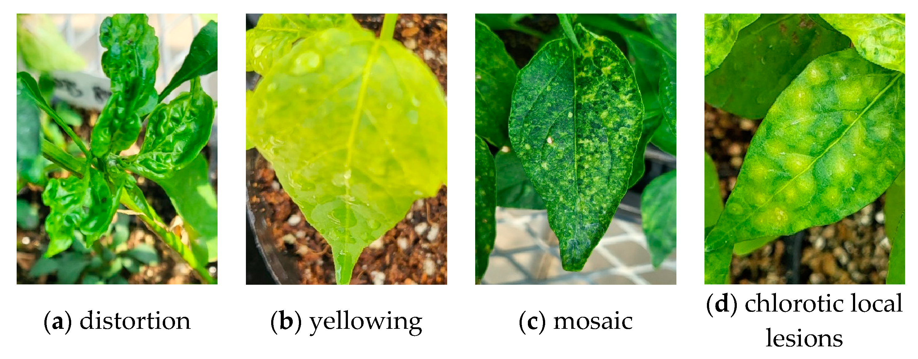
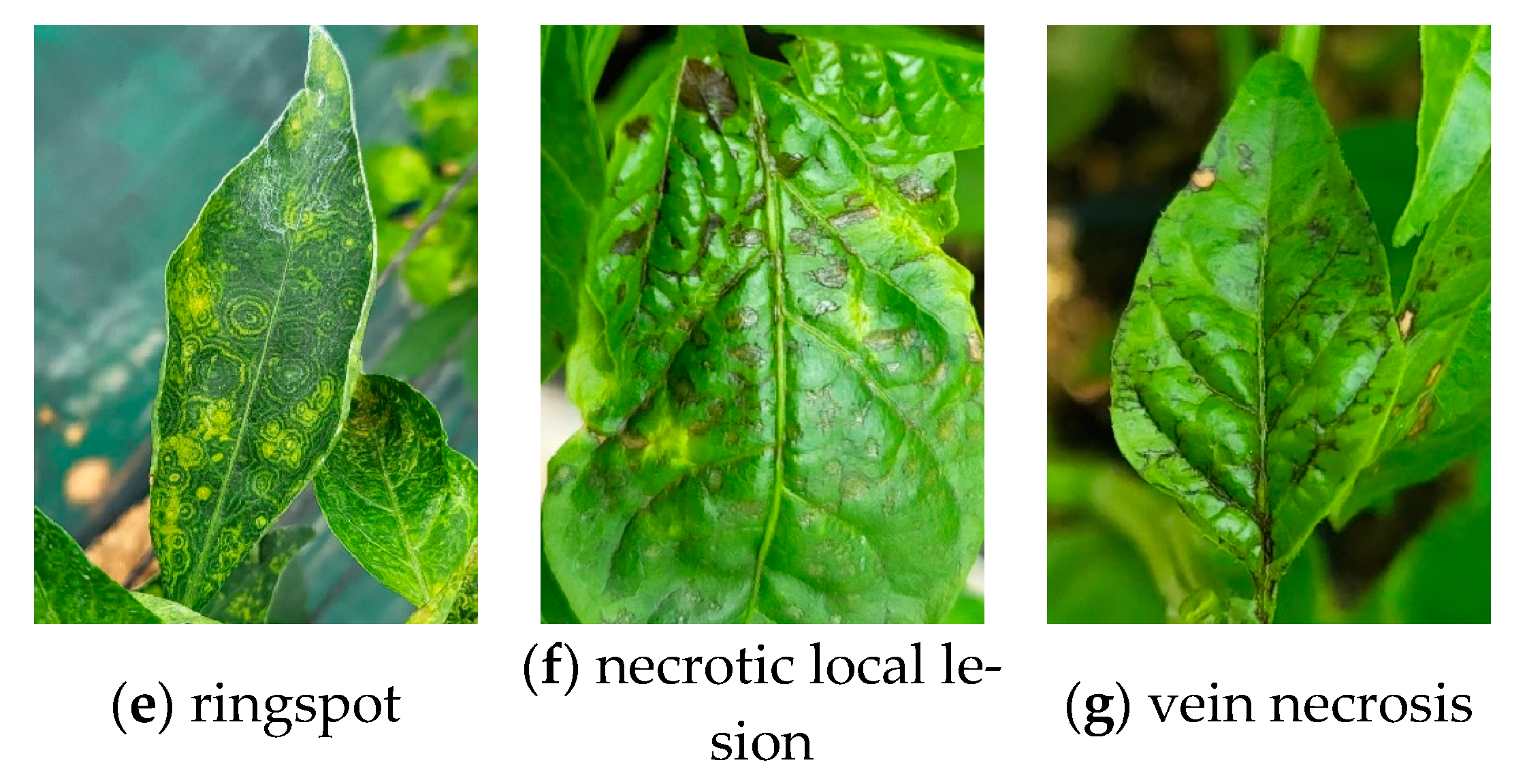
2.2. Tomato Spotted Wilt Virus (TSWV) Symptoms

Figure 2 shows typical symptoms that appear when infected with TSWV.

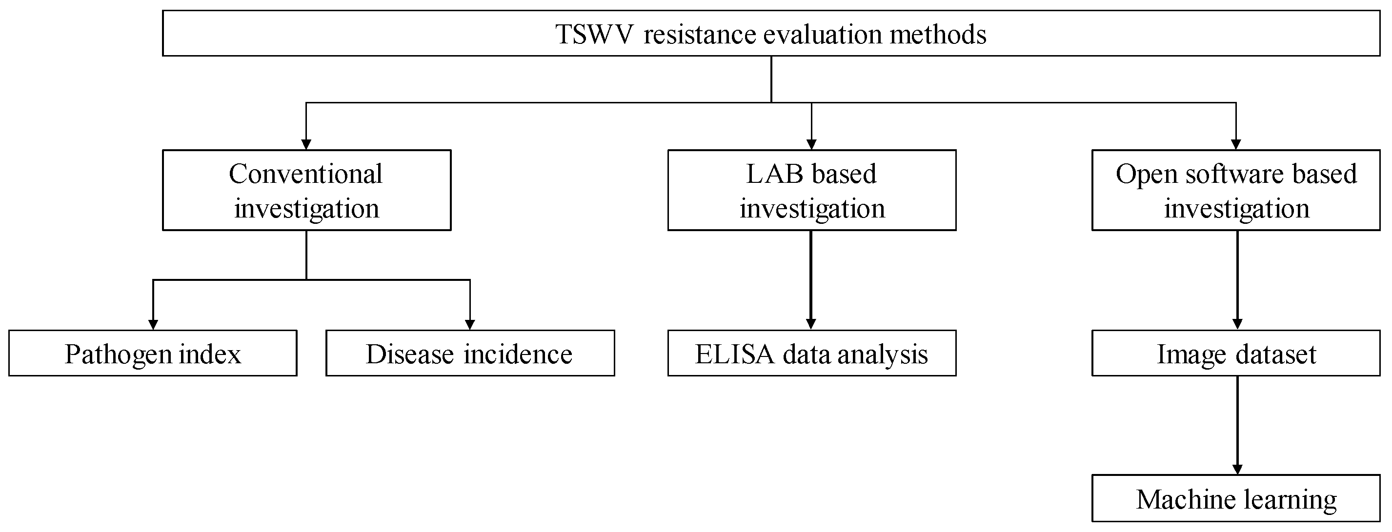
2.3. Conventional Investigation

A visual survey measured the pathogen index and disease incidence. The pathogen index evaluates the severity of the virus, while disease incidence assesses the extent of the virus spread. The pathogen index was assessed by visually evaluating symptoms recorded 28 days after inoculation, using a scale from 1 (no symptoms) to 5 (severe necrosis and stunting). Researchers investigated disease incidence by calculating the percentage of plants displaying symptoms after 28 days. If virus symptoms are present, the palnt is judged as S (Susceptible), and if there are no symptoms, it is judged as R (Resistant) (Figure 3).

Remark I. Pathogen indexing method

Tomato spotted wilt virus (TSWV) pathogen index:

1: No disease;

2: Weak apical leaf distortion;

3: Top distortion and weak mosaic in the older leaves;

4: Strong top leaf distortion, apical necrosis, and clear mosaic symptoms in the older leaves;

5: Severe stunting; top distortion and general necrosis.

2.4. LAB Based Investigation (ELISA)

ELISA (enzyme-linked Immunosorbent Assay) is a technique that measures color changes based on antigen–antibody reactions where antigens and antibodies bind. In this method, antigens and antibodies bind to change color, which is measured by a reader. If the color intensity exceeds a certain value (twice that of the negative control), it is considered infected. When a leaf (antigen) inoculated with TSWV (tomato spotted wilt virus) is crushed and placed on an ELISA plate coated with antibodies, binding occurs through the antigen–antibody reaction. At this time, the leaves that are not infected with TSWV do not bind. After washing with a buffer, ECA (enzyme-linked antibody) is added, and ECA binds to TSWV alkaline phosphatase (AP). This causes binding to the TSWV antigen. After washing eight times, PNP (para-nitrophenyl phosphate) substrate is added. This substrate is broken down by AP into para-nitrophenol, which turns yellow at 405 nm. The leaves infected with TSWV turn yellow and are determined to be infected with TSWV if the value measured by a spectrophotometer is more than twice that of the control. Following a visual survey and image capture, ELISA was performed to confirm TSWV infection. The upper leaves, rather than the inoculated leaves, were sampled for ELISA using a double antibody sandwich (DAS) ELISA kit (KisanBio, Seoul, Republic of Korea). The ELISA procedure followed the manufacturer’s instructions, and the infection status was determined by measuring absorbance at 405 nm. Samples with absorbance values more than twice that of healthy leaf samples were considered infected.

2.5. Open Software Based Investigation

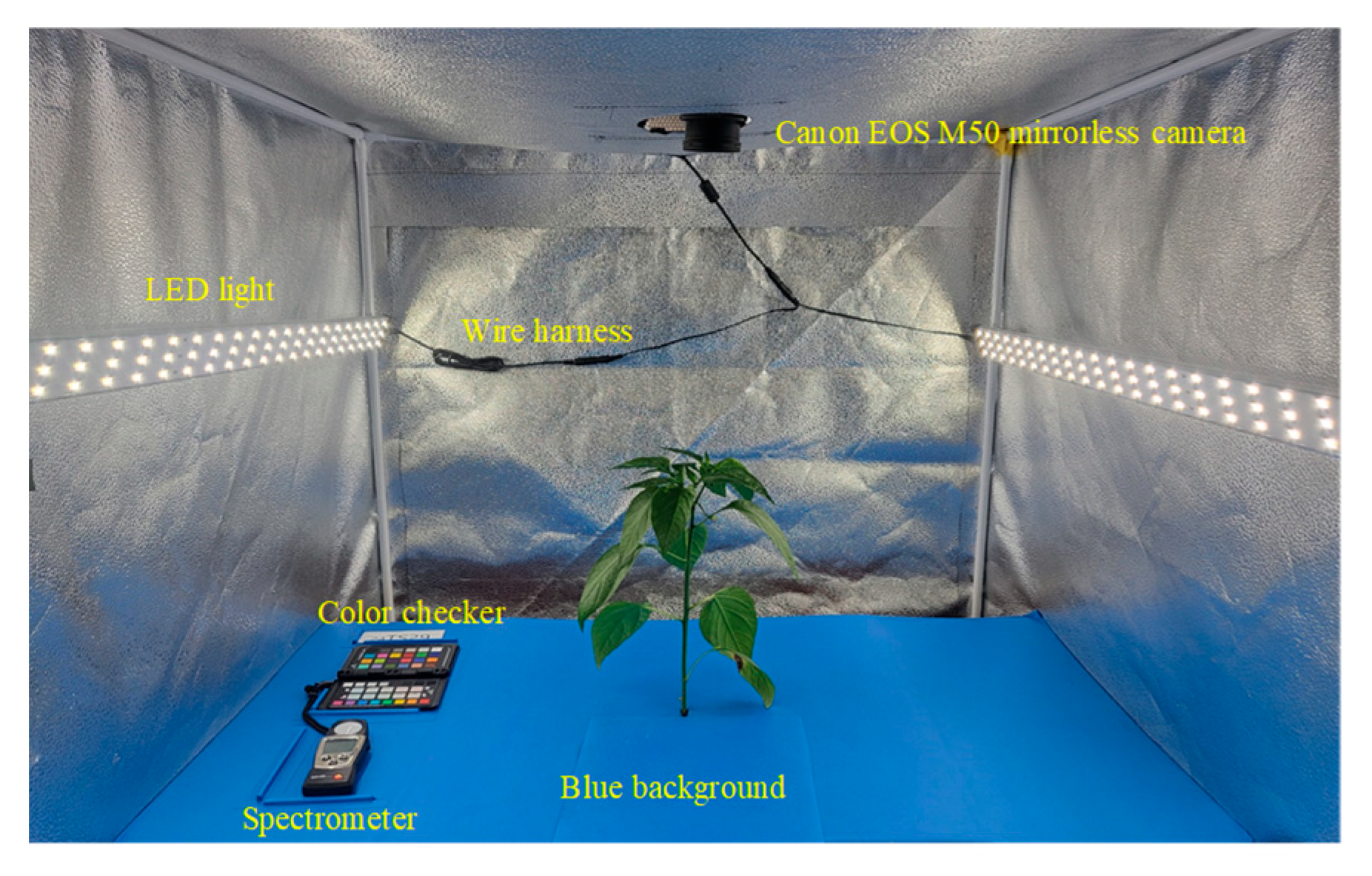
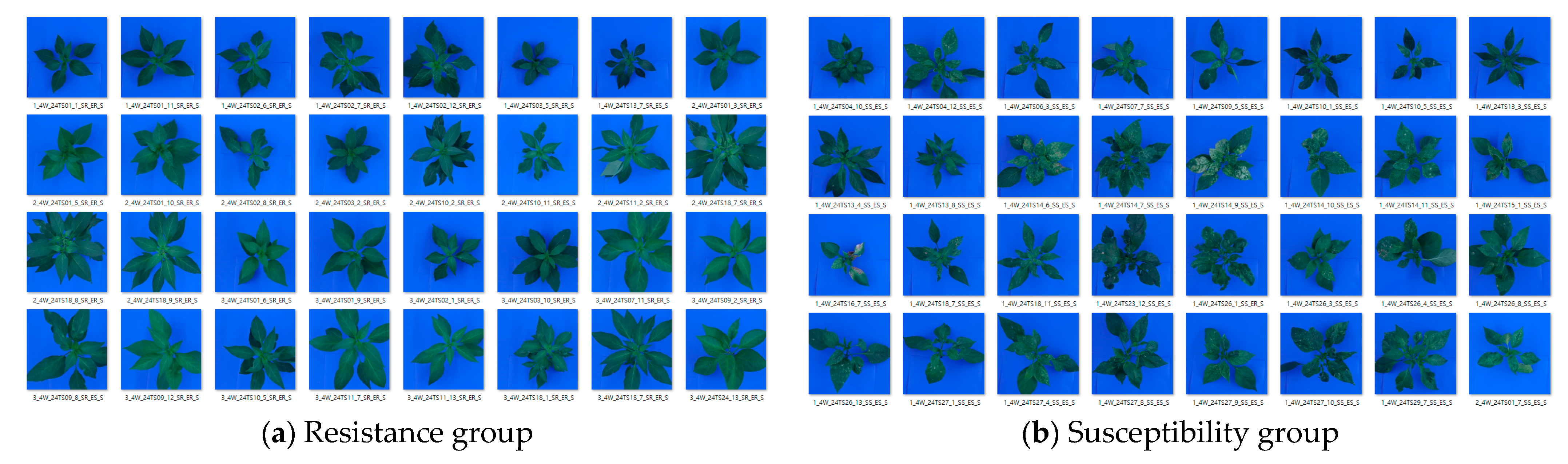
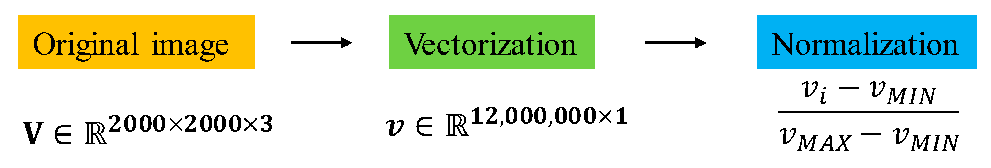
2.5.1. Image Dataset Collection

Figure 4 shows the LED light box used in this study for acquiring RGB data.

The image data generation process is as follows: 1. Turn on the light. 2. Check the illuminance inside the box using a spectrometer. 3. Acquire a color checker image to check the quality of the image data. The color checker is for calibration. 4. Acquire an image of the plant object.

To achieve reliable RGB image acquisition, uniform lighting, minimization of shadows and reflections, and color temperature and brightness adjustment are required. In this study, a preliminary test was conducted to obtain uniform RGB data of red peppers, and the light box was equipped with a blue background effective for RGB imaging.

The EOS M50 mirrorless camera (Canon Inc., Tokyo, Japan) for RGB data measurement features an approximately 24.1-megapixel resolution, touchscreen LCD, Full HD video resolution, MP4 video format, DIGIC 8 image processor (Budapest, Hungary), Dual Pixel CMOS AF autofocus, Wi-Fi and Bluetooth wireless connectivity, and a variety of interfaces. Color checkers and spectrometers assist with color correction. Each image has a resolution of 6000 × 3368 (72 dpi).

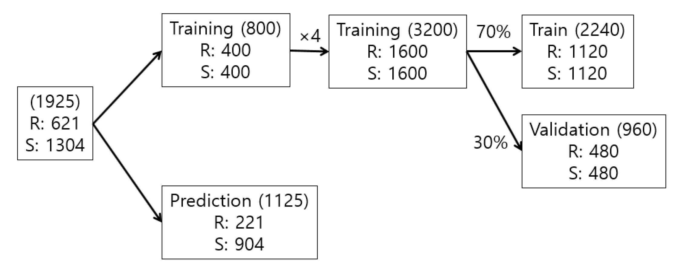
2.5.2. Image Data Usage Scheme

In this work, 1925 images were collected and manually segmented into two groups: the resistance group and the susceptibility group (Figure 5 and Figure 6). Next, 800 original photos were augmented as 3200 images, with 70% of them used for training and the remainder for validation. Using the developed models, 1125 images were predicted as follows.

Figure 7 shows the preprocessing for machine learning on the collected image data. The original image data has a three-dimensional tensor structure, which does not directly apply to the machine learning library used in this study. We converted the 3-dimensional tensor data into 1-dimensional vector data, normalized them, saved them in CSV file format, and applied them to the machine learning model.

2.5.3. Machine Learning

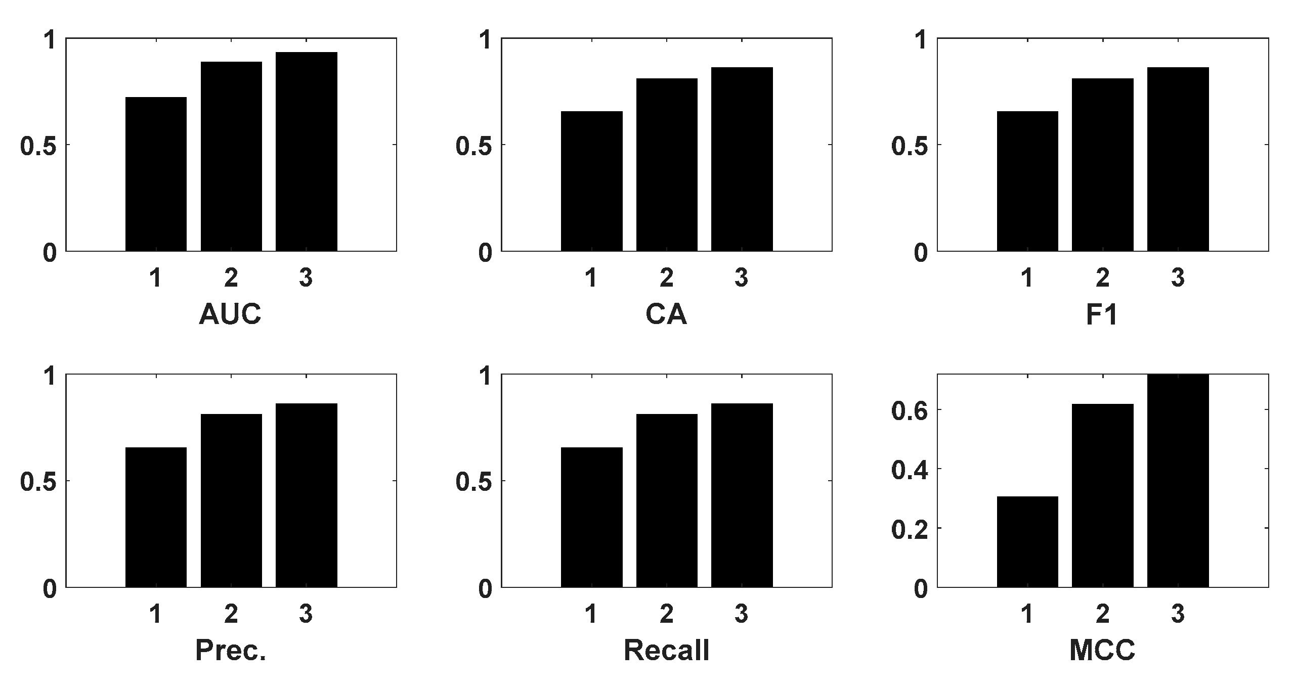
Machine-learning data are images taken at 15 dpi and 28 dpi. From three rounds of image capture, randomly select 400 images, each from TSWV-resistant and susceptible plants, totaling 800 images. Data augmentation technology improves model performance [9,10,24]. For simple geometric transformation, right-rotated, left-rotated, and vertically flipped images of the original photos were collected. The simulations for resistance determination were conducted using Orange3–3.36 software, employing models such as Support Vector Machine (SVM), Logistic Regression (LR), and neural networks (NNs). SVM is useful for finding complex boundaries, making it suitable for classification and regression, but it is computationally expensive for large datasets (Figure 8, Figure 9 and Figure 10). For agricultural applications of computer vision, it is important to have a method that is accessible to non-specialists. Orange Software was selected, as it meets this need effectively.

Early detection of plant diseases is necessary to improve the marketability of crops. Early diagnosis of plant diseases requires detailed investigation by experts, but it is time-consuming and expensive. Recently, computer vision has been in the spotlight as a means to replace this. A vision-based process for classifying image data is required to identify plant diseases. SVR, LR, and NN are classification algorithms with proven performance. Selecting algorithms with excellent performance is crucial for identifying plant diseases.

LR is mainly used for binary classification but has the disadvantage of low performance on non-linear data. NN models are suitable for pattern recognition and processing non-linear data in image and natural language processing, but they have the disadvantage of being slow in training and interpretation. The model with the highest accuracy was used to predict the disease resistance of an additional 1125 images not included in the training set.

2.5.4. Metrics

$$\mathrm{C}\mathrm{A}={\displaystyle \frac{\mathrm{T}\mathrm{P}+\mathrm{T}\mathrm{N}}{\mathrm{T}\mathrm{P}+\mathrm{F}\mathrm{N}+\mathrm{F}\mathrm{P}+\mathrm{T}\mathrm{N}}}$$

(1)

$$\mathrm{P}\mathrm{r}\mathrm{e}\mathrm{c}\mathrm{i}\mathrm{s}\mathrm{i}\mathrm{o}\mathrm{n}={\displaystyle \frac{\mathrm{T}\mathrm{P}}{\mathrm{T}\mathrm{P}+\mathrm{F}\mathrm{P}}}$$

(2)

$$\mathrm{R}\mathrm{e}\mathrm{c}\mathrm{a}\mathrm{l}\mathrm{l}={\displaystyle \frac{\mathrm{T}\mathrm{P}}{\mathrm{T}\mathrm{P}+\mathrm{F}\mathrm{N}}}$$

(3)

$$\mathrm{F}1 \mathrm{s}\mathrm{c}\mathrm{o}\mathrm{r}\mathrm{e}=2\times {\displaystyle \frac{\mathrm{P}\mathrm{r}\mathrm{e}\mathrm{c}\mathrm{i}\mathrm{s}\mathrm{i}\mathrm{o}\mathrm{n}\times \mathrm{R}\mathrm{e}\mathrm{c}\mathrm{a}\mathrm{l}\mathrm{l}}{\mathrm{P}\mathrm{r}\mathrm{e}\mathrm{c}\mathrm{i}\mathrm{s}\mathrm{i}\mathrm{o}\mathrm{n}+\mathrm{R}\mathrm{e}\mathrm{c}\mathrm{a}\mathrm{l}\mathrm{l}}}$$

(4)

$$\mathrm{M}\mathrm{C}\mathrm{C}={\displaystyle \frac{\mathrm{T}\mathrm{P}\times \mathrm{T}\mathrm{N}-\mathrm{F}\mathrm{P}\times \mathrm{F}\mathrm{N}}{\sqrt{(\mathrm{T}\mathrm{P}+\mathrm{F}\mathrm{P})(\mathrm{T}\mathrm{P}+\mathrm{F}\mathrm{N})(\mathrm{T}\mathrm{N}+\mathrm{F}\mathrm{P})(\mathrm{T}\mathrm{N}+\mathrm{F}\mathrm{N})}}}$$

(5)

where TP is true and positive, FP is false and positive, FN is false and negative, and TN is true and negative.

3. Results

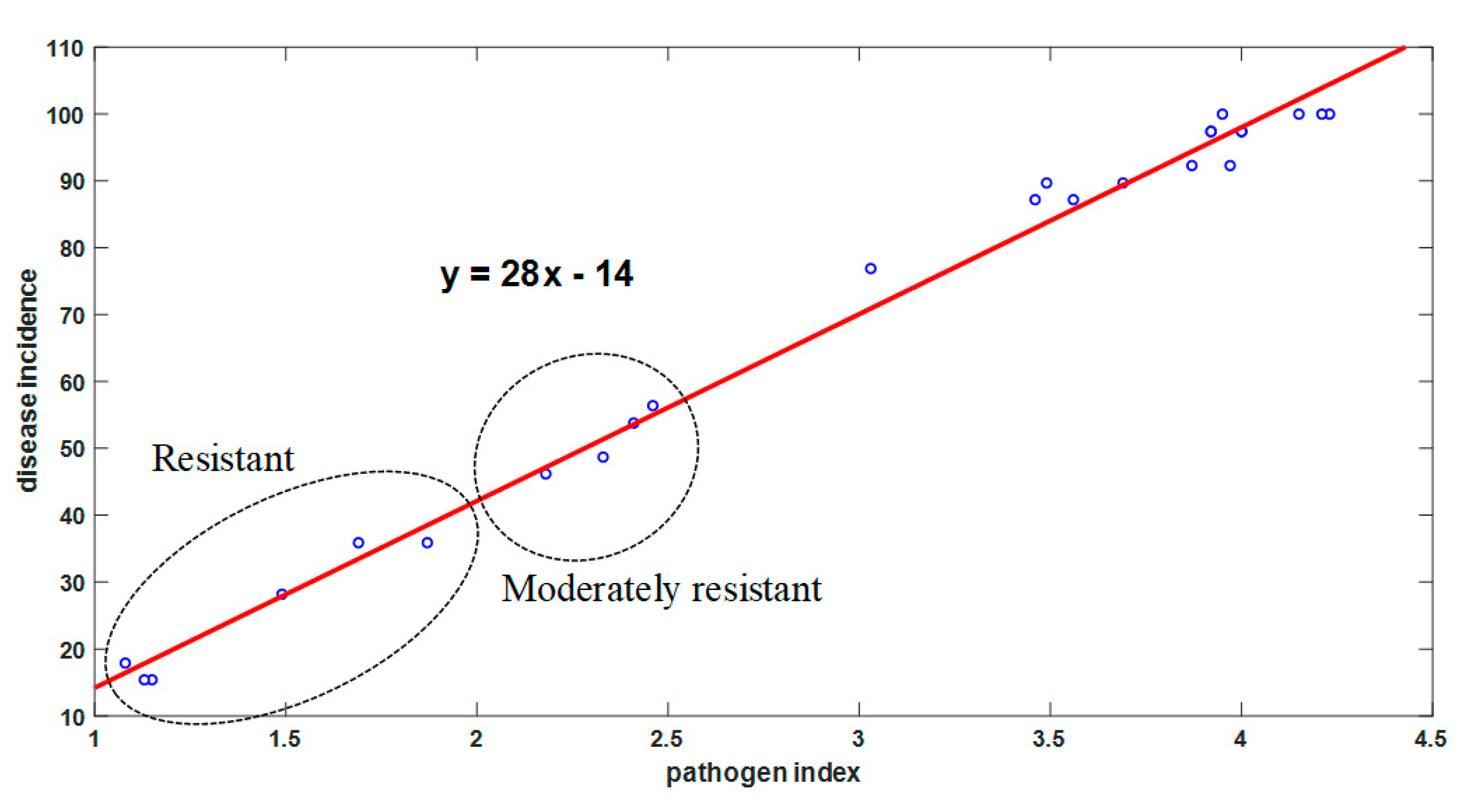
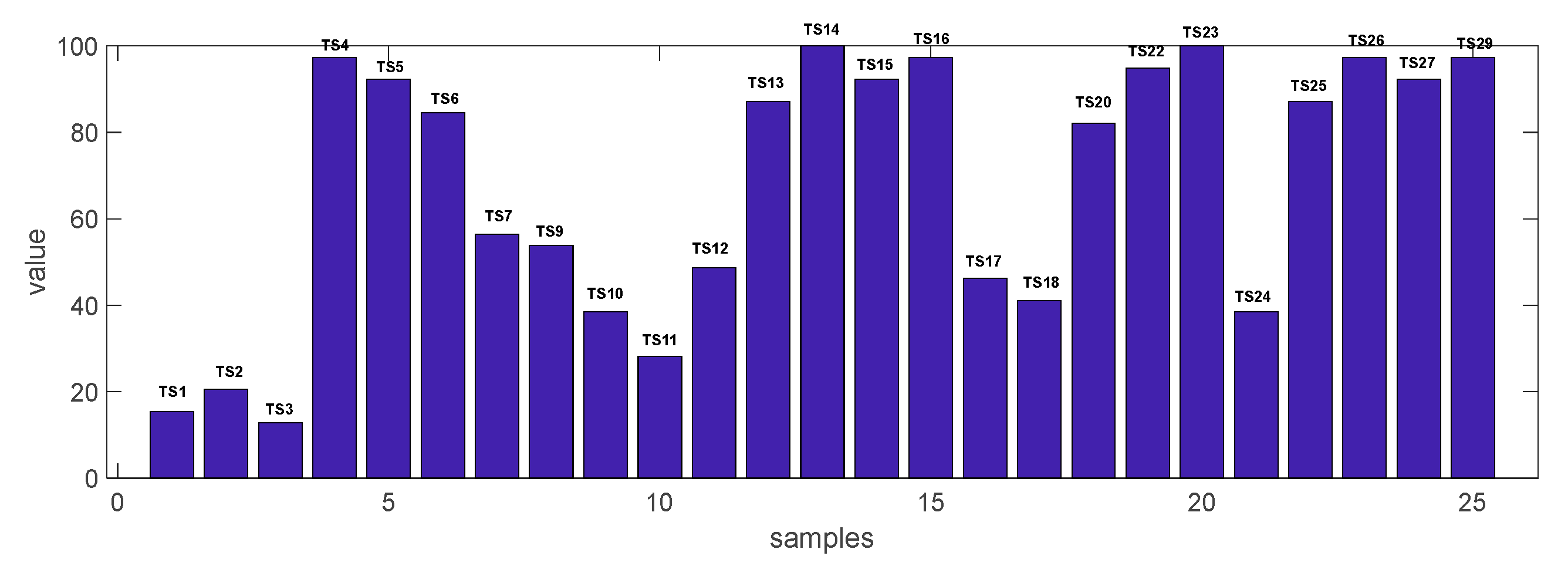
3.1. Resistance Determination

3.1.1. Conventional Investigation Results

Typical TSWV symptoms, such as mosaic patterns and circular spots, began to appear 9–10 days after inoculation. As the disease progressed, some lines exhibited stunted growth or plant death, while others showed no symptoms.

The lines with a pathogen index of 2.0 or lower were TS01, TS02, TS03, TS10, TS11, and TS24, totaling six lines. The lines with a disease incidence of 30% or lower were TS01, TS02, TS03, and TS24, totaling four lines showing resistance (Figure 11).

3.1.2. LAB-Based Investigation Results

ELISA analysis confirmed TSWV infection status, consistent with visual observations. TSWV antigen detection was minimal in resistant lines, whereas susceptible lines showed high antigen levels. Among the 21 candidate lines inoculated with the TSWV-P1 variant, three lines (TS01, TS02, and TS03) exhibited a disease incidence of 20% or lower, classifying them as resistant. Additionally, three lines (TS10, TS11, and TS24) exhibited a disease incidence of 40% or lower, categorizing them as moderately resistant. These lines showed a clear distinction in resistance compared to the susceptible control varieties (TS25, TS26, TS27, TS29). The control varieties had disease indices above 3.4 and incidences over 89% (Figure 12).

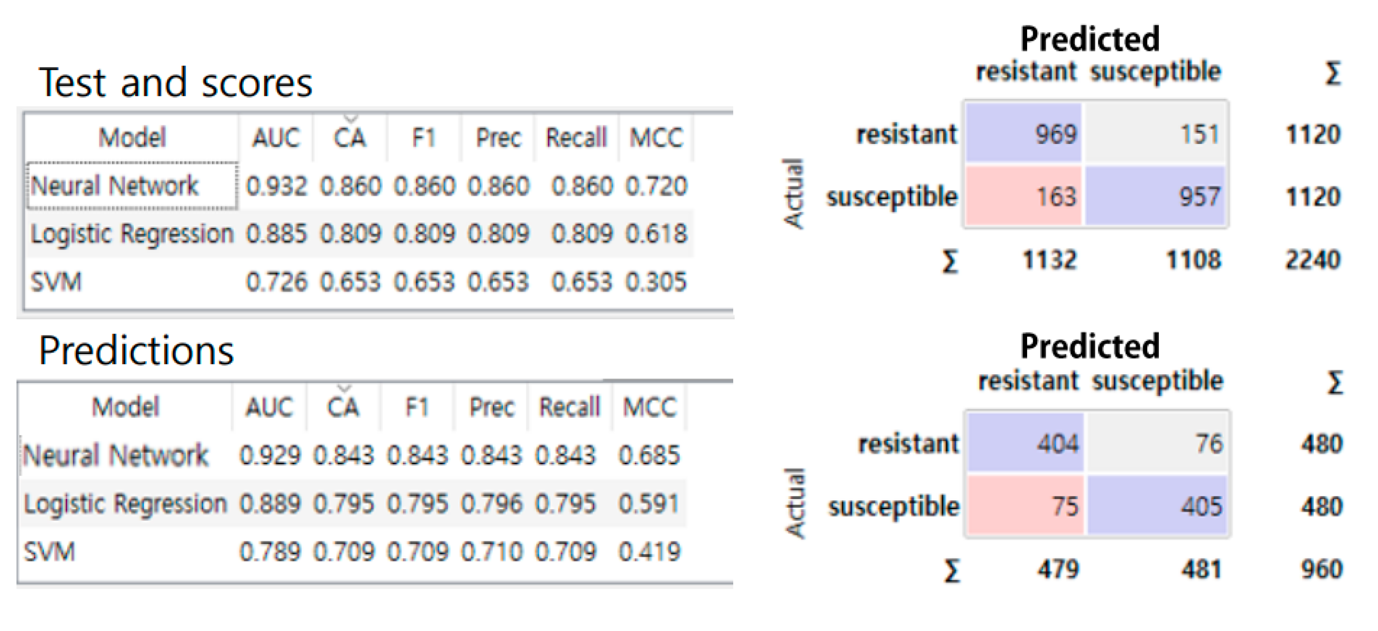
3.1.3. Machine Learning

The NN model exhibited the highest prediction accuracy, with a Classification Accuracy (CA) value of 0.860, significantly outperforming the LR and SVM models, which had CA values of 0.809 and 0.653, respectively (Figure 13). The NN model also demonstrated superior performance in Area Under the ROC Curve (AUC), Precision, Recall, and F1 Score, highlighting its robustness in classifying TSWV resistance.

Based on modeling performance, the superiority of the NN model was confirmed. Next, the prediction performance of the NN model was verified. As a result, in the validation set of 960 images not used for training, the NN model also achieved the highest prediction accuracy, with a CA of 0.843. Using the developed model, TSWV infection was predicted for the remaining 1125 images. Among the neural network (NN), Logistic Regression (LR), and Support Vector Machine (SVM) models, the neural network model showed the highest classification accuracy, at 0.829 (Figure 10).

3.2. Causality of Analytical Methods

Causality analysis uses statistical methods to examine the causal relationships among the three presented methods. The relationship between the classical method and ELISA was analyzed first, followed by an analysis of the relationship between ELISA and the NN method.

Table 1. Disease index and disease incidence of pepper line inoculated with tomato spotted wilt virus.

Germplasm	Pathogen Index z		Disease Incidence y		ELISA x		Machine Learning w
TS1	1.15 ± 0.61	a	15.4 ± 6.3	a	15.4 ± 6.3	ab	20.51 ± 7.3	a
TS2	1.13 ± 0.64	a	15.4 ± 6.3	a	20.5 ± 9.6	a–c	15.4 ± 10.9	a
TS3	1.08 ± 0.91	a	17.9 ± 25.4	ab	12.8 ± 18.1	a	28.2 ± 13.1	a
TS4	3.92 ± 0.11	fe	97.4 ± 3.6	g	97.4 ± 3.6	f	94.9 ± 7.3	d
TS5	3.87 ± 0.24	ef	92.3 ± 10.9	fg	92.3 ± 10.9	f	82.4 ± 15.4	d
TS6	3.56 ± 0.26	ef	87.2 ± 9.6	e–g	84.6 ± 10.9	ef	76.9 ± 18.8	cd
TS7	2.46 ± 0.38	b–d	56.4 ± 18.1	c–f	56.4 ± 18.1	ed	46.2 ± 21.8	a–c
TS9	2.33 ± 0.67	bc	48.7 ± 25.4	a–d	53.8 ± 25.1	c–e	23.1 ± 21.8	a
TS10	1.69 ± 0.35	ab	35.9 ± 22.1	a–c	38.5 ± 21.8	a–d	15.4 ± 16.6	a
TS11	1.87 ± 0.31	ab	35.9 ± 18.1	a–c	28.2 ± 18.1	a–d	28.2 ± 7.3	a
TS12	2.41 ± 0.89	c–d	53.8 ± 33.2	b–e	48.7 ± 28.3	b–d	46.2 ± 28.8	a–c
TS13	3.46 ± 0.51	d–f	87.2 ± 13.1	e–g	87.2 ± 9.6	ef	66.7 ± 15.8	b–d
TS14	4.15 ± 0.11	ef	100 ± 0.0	g	100 ± 0.0	f	94.9 ± 7.3	d
TS15	4.23 ± 0.19	fe	100 ± 0.0	g	92.3 ± 6.3	f	97.4 ± 3.6	d
TS16	4.00 ± 0.11	ef	97.4 ± 3.6	g	97.4 ± 3.6	f	94.7 ± 3.8	d
TS17	3.03 ± 0.73	c–d	76.9 ± 22.6	d–g	46.2 ± 28.8	a–d	69.2 ± 22.6	b–d
TS18	2.18 ± 0.67	a–c	46.2 ± 28.8	a–d	41.0 ± 26.1	a–d	43.6 ± 23.8	ab
TS20	3.97 ± 0.35	ef	92.3 ± 6.3	fg	82.1 ± 9.6	ef	82.2 ± 13.7	d
TS22	4.21 ± 0.29	fe	100 ± 0.0	g	94.9 ± 7.3	f	94.9 ± 3.6	d
TS23	4.00 ± 0.13	ef	97.4 ± 3.6	g	100 ± 0.0	f	85.9 ± 14.1	d
TS24	1.49 ± 0.80	ab	28.2 ± 25.4	a–c	38.5 ± 22.6	a–d	17.9 ± 13.1	a
TS25	3.49 ± 0.44	d–f	89.7 ± 14.5	e–g	87.2 ± 9.6	ef	79.5 ± 3.6	d
TS26	3.95 ± 0.07	ef	100 ± 0.0	g	97.4 ± 3.6	f	94.9 ± 3.6	d
TS27	3.69 ± 0.44	ef	89.7 ± 14.5	e–g	92.3 ± 10.9	f	92.3 ± 10.9	d
TS29	3.92 ± 0.17	ef	97.4 ± 3.6	g	97.4 ± 3.6	f	89.7 ± 7.3	d

^z A quantitative measure of the disease severity on a scale from 1 (no symptoms) to 5 (severe necrosis and stunting). It is a visual evaluation of symptoms recorded 28 days after inoculation. ^y The percentage of plants that showed symptoms of the disease after 28 days. ^x The infection rate was determined 28 days after inoculation using ELISA testing. ^w Predictive values from a neural network model about the infection rates after 28 days. Values followed by the same letter within a column are not significantly different at p = 0.01 according to Duncan’s multiple range test.

depicts this analysis. Each entry in the table also includes standard deviations and statistical grouping (denoted by letters). Values followed by the same letter within a column are not significantly different at the 0.01 level according to Duncan’s multiple range test, indicating statistical grouping and comparison of means.

3.2.1. Average Causality

The conventional method includes columns 1 and 2 of Table 1. The ELISA data analysis results were confirmed to be closely related to the pathogen index and disease incidence.

$${\mathrm{\epsilon }}_{\mu }=26.8{\mathrm{\alpha }}_{\mu }-12.6(\mathrm{R}2=0.94,p<0.05)$$

(6)

$${\mathrm{\epsilon }}_{\mu }=0.95{\mathrm{\beta }}_{\mu }+0.85(\mathrm{R}2=0.94,p>0.05)$$

(7)

where ${\mathrm{\epsilon }}_{\mathsf{\mu }}$ is the average of ELISA, ${\mathrm{\alpha }}_{\mathsf{\mu }}$ is the average of the pathogen index, ${\mathrm{\beta }}_{\mathsf{\mu }}$ is the average of the disease incidence.

Next, the relationship between ELISA and NN was conducted as follows.

$${\mathrm{\epsilon }}_{\mu }=0.92{\mathrm{\gamma }}_{\mu }+9.8(\mathrm{R}2=0.86,p<0.05)$$

(8)

3.2.2. STD Causality

$${\mathrm{\epsilon }}_{\sigma }=26.5{\mathrm{\alpha }}_{\sigma }+1.5(\mathrm{R}2=0.59,p>0.05)$$

(9)

$${\mathrm{\epsilon }}_{\sigma }=0.8{\mathrm{\beta }}_{\sigma }+2.2(\mathrm{R}2=0.87,p<0.05)$$

(10)

$${\mathrm{\epsilon }}_{\sigma }=0.93{\mathrm{\gamma }}_{\sigma }+0.7(\mathrm{R}2=0.58,p>0.05)$$

(11)

where ${\mathrm{\epsilon }}_{\sigma }$ is the standard deviation of ELISA, ${\mathrm{\alpha }}_{\sigma }$ is the standard deviation of the pathogen index, ${\mathrm{\beta }}_{\sigma }$ is the standard deviation of the disease incidence, and ${\mathrm{\gamma }}_{\sigma }$ is the standard deviation of the NN model.

4. Discussion

4.1. Interpretation of Causality Analysis Results

Table 2. Summary of causality results.

Metrics	Pathogen Index	Disease Incidence	NN Model
mean	significant	insignificant	significant
standard deviation	insignificant	insignificant	insignificant

shows the summary of the causality analysis results.

The three methods presented demonstrated a strong correlation with each other, but the statistically significant causal relationships were the pathogen index, ELISA, and the NN model.

4.2. Practical Scenarios

TSWV is an RNA virus with a high mutation rate during replication, allowing it to rapidly adapt to new environments or hosts [25]. Numerous reports have documented TSWV resistance-breaking strains in pepper [26,27,28,29,30]. The high mutation rate of TSWV, the complexity of resistance mechanisms, and the difficulty in identifying genes that provide durable resistance limit the commercial development of TSWV-resistant cultivars. By appropriately utilizing each method presented in this study, a reselection system for varieties that can respond quickly and accurately to mutations can be established.

The advantages and disadvantages of the presented three methods can be summarized as follows (

Table 3. Summary of the three methods.

	Visual	ELISA	Neural Network
advantages	simple	sensitive	accurate
disadvantages	inaccurate	complex and expensive	difficult

).

Depending upon the situation in which a mutation occurs, the following methods of use are recommended.

• Signs of mutation occur (macroscopic evaluation by visual inspection);
• Variety selection process based on initial mutation occurrence (micro-evaluation by ELISA);
• Continuous monitoring according to the spread of mutations (evaluation of mutation trends by open software).

As virus mutations spread, analysis and evaluation trends are required. Although NN-ELISA did not provide generalized results for distributed data in this study, statistical causality will be able to be established in the future by securing high-quality datasets and applying accurate and precise ELISA analysis techniques. Therefore, machine learning methods are necessary for analyzing virus fluctuation trends.

4.3. Performance Comparison

Hyperspectral images are an effective tool for analyzing crop images based on ma-chine learning [6]. The latest hyperspectral image-based crop disease detection accuracies have been reported to range from 59% to 79.2%. The accuracy level of crop disease detection can vary greatly depending on the algorithm used. These research results were similar to the accuracy level variability of the three algorithms used in this study. However, hyperspectral imaging has high hardware costs and complex data processing. RGB-based machine learning may provide a more efficient solution for identifying crop diseases.

5. Conclusions

State-of-the-art techniques for assessing TSWV resistance in tomatoes include visual inspection, ELISA assays, and imaging and machine-learning methods. The proposed imaging and machine learning-based assessment approaches hold significant potential to advance sustainable agriculture by conserving environmental resources and enhancing productivity. With the rapid progress in computational technology, the accuracy of disease resistance assessment methods is expected to improve, leading to the wider adoption of non-destructive techniques for determining disease resistance. It is necessary to use the proposed methods efficiently, based on research results. All three methods can, on average, serve as alternatives to address or predict the results of other methods. However, causal analysis methods that include standard deviation still lack generalization. The proposed NN model is for diagnosing the severity of virus variants ex post facto or selecting virus-resistant varieties through variant reassessment, but the spread of variants is not generalized. Developing advanced and statistically generalized techniques that can accurately assess both aspects simultaneously remains a research challenge.

References

1. Altizani-Júnior, J.C.; Cicero, S.M.; de Lima, C.B.; Alves, R.M.; Gomes-Junior, F.G. Optimizing basil seed vigor evaluations: An automatic approach using computer vision-based technique. Horticulturae 2024, 10, 1220. [Google Scholar] [CrossRef]
2. Fuentes-Peñailillo, F.; Carrasco Silva, G.; Pérez Guzmán, R.; Burgos, I.; Ewertz, F. Automating seedling counts in horticulture using computer vision and AI. Horticulturae 2023, 9, 1134. [Google Scholar] [CrossRef]
3. Zhang, W.; Dang, L.M.; Nguyen, L.Q.; Alam, N.; Bui, N.D.; Park, H.Y.; Moon, H. Adapting the segment anything model for plant recognition and automated phenotypic parameter measurement. Horticulturae 2024, 10, 398. [Google Scholar] [CrossRef]
4. García-Amaro, E.; Cervantes-Canales, J.; García-Lamont, F.; Lara-Viveros, F.M.; Ruiz-Castilla, J.S.; Espejel Cabrera, J. Use of computer vision techniques for recognition of diseases and pasts in tomato plants. Comput. Sist. 2024, 28, 709–723. [Google Scholar] [CrossRef]
5. Clohessy, J.W.; Sanjel, S.; O’Brien, G.K.; Barocco, R.; Kumar, S.; Adkins, S.; Tillman, B.; Wright, D.L.; Small, I.M. Development of a high-throughput plant disease symptom severity assessment tool using machine learning image analysis and integrated geolocation. Comput. Electron. Agric. 2021, 184, 106089. [Google Scholar] [CrossRef]
6. García-Vera, Y.E.; Polochè-Arango, A.; Mendivelso-Fajardo, C.A.; Gutiérrez-Bernal, F.J. Hyperspectral image analysis and machine learning techniques for crop disease detection and identification: A review. Sustainability 2024, 16, 6064. [Google Scholar] [CrossRef]
7. Ahmad, A.; Saraswat, D.; El Gamal, A. A survey on using deep learning techniques for plant disease diagnosis and recommendations for development of appropriate tools. Smart Agric. Technol. 2023, 3, 100083. [Google Scholar] [CrossRef]
8. Braga, P.; Crusiol, L.G.T.; Nanni, M.R.; Caranhato, A.L.H.; Fuhrmann, M.B.; Nepomuceno, A.L.; Neumaier, N.; Farias, J.R.B.; Koltun, A.; Gonçalves, L.S.A.; et al. Vegetation indices and NIR-SWIR spectral bands as a phenotyping tool for water status determination in soybean. Precis. Agric. 2021, 22, 249–266. [Google Scholar] [CrossRef]
9. Lee, S.-D.; Gil, C.-S.; Lee, J.-H.; Jeong, H.-B.; Kim, J.-H.; Jang, Y.-A.; Kim, D.-Y.; Lee, W.-M.; Moon, J.-H. Internal quality prediction technology for ‘Sulhyang’ strawberry fruit using organic analysis and hyperspectral imaging. Spectrochim. Acta Part A 2024, 323, 124912. [Google Scholar] [CrossRef] [PubMed]
10. Lee, S.-D.; Lee, J.-H.; Kim, J.-H.; Jang, Y.-a.; Moon, J.-H. Evaluation technologies for assessing drought tolerance of Kimchi cabbage seedlings using hyperspectral imaging and principal component analysis. Microchem. J. 2024, 206, 111499. [Google Scholar] [CrossRef]
11. Kamilaris, A.; Prenafeta-Boldú, F.X. Deep learning in agriculture: A survey. Comput. Electron. Agric. 2018, 147, 70–90. [Google Scholar] [CrossRef]
12. Lafrance, R.; Villicaña, C.; Valdéz-Torres, J.B.; García-Estrada, R.S.; Báez Sañudo, M.A.; Esparza-Araiza, M.J.; León-Félix, J. Selection of tomato (Solanum lycopersicum) Hybrids Resistant to Fol, TYLCV, and TSWV with early maturity and good fruit quality. Horticulturae 2024, 10, 839. [Google Scholar] [CrossRef]
13. Oh, B.G.; Chung, J.-S.; Ju, H.-J.; Yoon, J.Y.; Baek, E. Arctium lappa is a new natural host of Tomato spotted wilt virus in Korea. Plant Dis. 2024, 108, 3206. [Google Scholar] [CrossRef] [PubMed]
14. Abdisa, E.; Kwon, J.; Jin, G.; Kim, Y. Thrips and TSWV occurrence in geographically different open fields cultivating hot peppers. Korean J. Appl. Entomol. 2024, 63, 43–51. [Google Scholar] [CrossRef]
15. Shymanovich, T.; Saville, A.C.; Mohammad, N.; Wei, Q.; Rasmussen, D.; Lahre, K.A.; Rotenberg, D.; Whitfield, A.E.; Ristaino, J.B. Disease progress and detection of a california resistance-breaking strain of Tomato spotted wilt virus in tomato with LAMP and CRISPR-Cas12a assays. PhytoFrontiers 2024, 4, 50–60. [Google Scholar] [CrossRef]
16. Juárez, I.D.; Steczkowski, M.X.; Chinnaiah, S.; Rodriguez, A.; Gadhave, K.R.; Kurouski, D. Using Raman spectroscopy for early detection of resistance-breaking strains of tomato spotted wilt orthotospovirus in tomatoes. Front. Plant Sci. 2024, 14, 1283399. [Google Scholar] [CrossRef]
17. Caruso, A.G.; Ragona, A.; Agrò, G.; Bertacca, S.; Yahyaoui, E.; Galipienso, L.; Rubio, L.; Panno, S.; Davino, S. Rapid detection of tomato spotted wilt virus by real-time RT-LAMP and in-field application. J. Plant Pathol. 2024, 106, 697–712. [Google Scholar] [CrossRef]
18. Jahn, M.; Paran, I.; Hoffmann, K.; Radwanski, E.R.; Livingstone, K.D.; Grube, R.C.; Aftergoot, E.; Lapidot, M.; Moyer, J. Genetic mapping of the Tsw locus for resistance to the Tospovirus Tomato spotted wilt virus in Capsicum spp. and its relationship to the Sw-5 gene for resistance to the same pathogen in tomato. Mol. Plant-Microbe Interact. 2000, 13, 673–682. [Google Scholar] [CrossRef]
19. Parisi, M.; Alioto, D.; Tripodi, P. Overview of botic stresses in pepper (Capsicum spp.): Sources of genetic resistance, molecular breeding and genomics. Int. J. Mol. Sci. 2020, 21, 2587. [Google Scholar] [CrossRef]
20. Roggero, P.; Masenga, V.; Tavella, L. Field isolates of Tomato spotted wilt virus overcoming resistance in pepper and their spread to other hosts in Italy. Plant Dis. 2002, 86, 950–954. [Google Scholar] [CrossRef] [PubMed]
21. Yoon, J.Y.; Her, N.H.; Cho, I.S.; Chung, B.N.; Choi, S.K. First report of a resistance-breaking strain of Tomato spotted wilt orthotospovirus infecting Capsicum annuum carrying the Tsw resistance gene in South Korea. Plant Dis. 2021, 105, 2259. [Google Scholar] [CrossRef]
22. Han, J.-H.; Lee, W.-P.; Lee, J.-D.; Kim, M.-K.; Choi, H.-S.; Yoon, J.-B. Symptom and resistance of cultivated and wild Capsicum accessions to Tomato spotted wilt virus. Res. Plant Dis. 2011, 17, 59–65. [Google Scholar] [CrossRef]
23. Liu, J.; Wang, X. Plant diseases and pests detection based on deep learning: A review. Plant Methods 2021, 17, 22. [Google Scholar] [CrossRef] [PubMed]
24. Taylor, L.; Nitschke, G. Improving deep learning with generic data augmentation. In Proceedings of the 2018 IEEE Symposium Series on Computational Intelligence (SSCI), Bangalore, India, 18–21 November 2018; pp. 1542–1547. [Google Scholar]
25. Duffy, S. Why are RNA virus mutation rates so damn high? PLoS Biol. 2018, 16, e3000003. [Google Scholar] [CrossRef] [PubMed]
26. Ciuffo, M.; Finetti-Sialer, M.M.; Gallitelli, D.; Turina, M. First report in Italy of a resistance-breaking strain of Tomato spotted wilt virus infecting tomato cultivars carrying the Sw5 resistance gene. Plant Pathol. 2005, 54, 564. [Google Scholar] [CrossRef]
27. Deligoz, I.; Sokmen, M.A.; Sari, S. First report of resistance breaking strain of Tomato spotted wilt virus (Tospovirus; Bunyaviridae) on resistant sweetpepper cultivars in Turkey. New Dis. Rep. 2014, 30, 26. [Google Scholar] [CrossRef]
28. Orecchio, C.; Sacco Botto, C.; Alladio, E.; D’Errico, C.; Vincenti, M.; Noris, E. Non-invasive and early detection of tomato spotted wilt virus infection in tomato plants using a hand-held Raman spectrometer and machine learning modelling. Plant Stress 2025, 15, 100732. [Google Scholar] [CrossRef]
29. Macedo, M.A.; Rojas, M.R.; Gilbertson, R.L. First report of a resistance-breaking strain of tomato spotted wilt orthotospovirus infecting sweet pepper with the Tsw resistance gene in California, U.S.A. Plant Dis. 2019, 103, 1048. [Google Scholar] [CrossRef]
30. Ferrand, L.; Almeida, M.M.S.; Orílio, A.F.; Dal Bó, E.; Resende, R.O.; García, M.L. Biological and molecular characterization of tomato spotted wilt virus (TSWV) resistance-breaking isolates from Argentina. Plant Pathol. 2019, 68, 1587–1601. [Google Scholar] [CrossRef]
Figure 1. Overall scheme of this study.
Horticulturae 11 00132 g001
Figure 2. TSWV symptoms. The main symptoms are as follows: (a) Distortion occurs where the leaf is twisted or bent. (b) Yellow spots appear on the leaves. (c) Patterns develop on the leaves. (d) Localized yellow lesions occur due to chlorophyll deficiency. (e) Circular spots occur. (f) Localized necrotic lesions occur. (g) Vascular necrosis occurs. The leaf veins and stem tissues die and turn black.
Horticulturae 11 00132 g002aHorticulturae 11 00132 g002b
Figure 3. Asymptomatic (a) and symptomatic (b) appearance.
Horticulturae 11 00132 g003
Figure 4. RGB image acquisition system.
Horticulturae 11 00132 g004
Figure 5. Image data usage scheme in this work.
Horticulturae 11 00132 g005
Figure 6. Classification according to the resistance to tomato spotted wilt virus (TSWV). Depending on the presence or absence of symptoms, they were classified as resistant or susceptible.
Horticulturae 11 00132 g006
Figure 7. Image preprocessing where V is a tensor, v is a vector, v i is a scalar for a specific feature i , v M A X is a maximum value of features, and v M I N is a minimum value of features.
Horticulturae 11 00132 g007
Figure 8. Open software Orange3–3.36-based workflow with training and validation used in this study. The images are divided, with 70% of them used for training and 30% used for validation. To classify TSWV resistance, we used various algorithms, such as Support Vector Machines (SVM), Logistic Regression, and neural networks.
Horticulturae 11 00132 g008
Figure 9. Model development and validation based on open software Orange3–3.36.
Horticulturae 11 00132 g009
Figure 10. Prediction performance evaluation based on open software Orange3–3.36.
Horticulturae 11 00132 g010
Figure 11. Selection results of resistant groups (R2 = 0.99, p < 0.05).
Horticulturae 11 00132 g011
Figure 12. ELISA data analysis results.
Horticulturae 11 00132 g012
Figure 13. Modeling performances. AUC is the area under the receiver operation characteristic curve, with a range of 0~1. CA, F1, Prec., Recall, and MCC are defined from (1) to (5), where 1 on the horizontal axis is LR, 2 is SVM, and 3 is NN.
Horticulturae 11 00132 g013