Article

Counterfeit Detection of Iranian Black Tea Using Image Processing and Deep Learning Based on Patched and Unpatched Images

by
Mohammad Sadegh Besharati
1,
Raziyeh Pourdarbani
1,*,
Sajad Sabzi
2,
Dorrin Sotoudeh
2,
Mohammadreza Ahmaditeshnizi
2 and
Ginés García-Mateos
3,*
1
Department of Biosystems Engineering, University of Mohaghegh Ardabili, Ardabil 56199-11367, Iran
2
Department of Computer Engineering, Sharif University of Technology, Tehran 14588-89694, Iran
3
Computer Science and Systems Department, University of Murcia, 30100 Murcia, Spain
*
Authors to whom correspondence should be addressed.
Horticulturae 2024, 10(7), 665; https://doi.org/10.3390/horticulturae10070665
Submission received: 21 May 2024 / Revised: 17 June 2024 / Accepted: 20 June 2024 / Published: 23 June 2024
(This article belongs to the Section Postharvest Biology, Quality, Safety, and Technology)

Abstract

:
Tea is central to the culture and economy of the Middle East countries, especially in Iran. At some levels of society, it has become one of the main food items consumed by households. Bioactive compounds in tea, known for their antioxidant and anti-inflammatory properties, have proven to confer neuroprotective effects, potentially mitigating diseases such as Parkinson’s, Alzheimer’s, and depression. However, the popularity of black tea has also made it a target for fraud, including the mixing of genuine tea with foreign substitutes, expired batches, or lower quality leaves to boost profits. This paper presents a novel approach to identifying counterfeit Iranian black tea and quantifying adulteration with tea waste. We employed five deep learning classifiers—RegNetY, MobileNet V3, EfficientNet V2, ShuffleNet V2, and Swin V2T—to analyze tea samples categorized into four classes, ranging from pure tea to 100% waste. The classifiers, tested in both patched and non-patched formats, achieved high accuracy, with the patched MobileNet V3 model reaching an accuracy of 95% and the non-patched EfficientNet V2 model achieving 90.6%. These results demonstrate the potential of image processing and deep learning techniques in combating tea fraud and ensuring product integrity in the tea industry.

1. Introduction

Since its inception, tea has been used as a traditional beverage to promote health and mental peace, as it contains compounds with antioxidant, anti-inflammatory, immune-enhancing, metabolic-regulating, and cytoprotective properties [1,2]. In addition to its unique taste, tea is rich in many bioactive compounds such as catechins, polyphenols, polysaccharides, polypeptides, pigments, and alkaloids, which are effective health factors [3,4,5]. In Iran, where this study was conducted, about 32,000 ha of farms in the northern part of the country is devoted to tea cultivation due to the suitable climatic conditions for its cultivation [6]. The most common and popular type of tea is black tea, which is plucked from green tea leaves and obtained after dehumidification, rubbing, fermentation, and drying [7,8,9].
However, food, as a fundamental human necessity, often becomes a target for fraudulent activities within its lucrative market. Fraudsters, driven by the prospect of substantial profits, may resort to various deceptive practices that can jeopardize public health [10]. Not all food fraud is intentional; some instances arise inadvertently due to negligence or inadequate hygiene standards during production [11]. Thus, it is crucial to identify and address food fraud due to its potential health, economic, social, and psychological impacts [12,13], including fraud in tea production.
The adulteration of black tea is a challenging problem due to its universality and popularity [14,15]. Among the major adulterations of tea, the following can be mentioned: mixing tea with similar foreign varieties but with large differences in economic value [16] or adding flavoring and coloring materials including pigments and other dyes to improve the appearance of tea or damaged tea leaves [17]. Some profiteers also offer tea waste in the form of high-quality tea with the addition of colorants and additives. Tea leaves may be mixed with sand, sawdust, and plant roots and marketed to increase volume and weight [18,19]. Even the very small amounts of iron shavings that are added during tea processing [20] happen to lower the final price and increase the profit margin of fraudulent producers.
There are several methods to detect food fraud. One of the most traditional methods is visual inspection, which is a very tedious and time-consuming task [21]. It is also highly dependent on the skill of the analyst and may not be suitable for all types of fraud. For tea, physical and microscopic examinations by trained technicians are proven approaches to detect foreign material. However, this is not a reliable method for distinguishing colors [22]. With advances in artificial intelligence technologies, the development and implementation of food quality control systems are becoming increasingly possible. There is potential to use various artificial intelligence programs such as machine learning models, natural language processing, and image processing to improve food safety [10]. Deep learning is a subset of machine learning that does not necessarily require a labeled dataset in the sense that it can use unsupervised learning for its training [23].
In the work of Xu et al. [24], deep learning techniques were used to distinguish high-quality tea from old tea; this approach showed its high potential in tea quality analysis using image processing. In another study by Amsaraj and Mutturi [25], a machine learning method was used to identify the artificial color added in tea to classify and determine the amount of fraud, and the result showed the potential of the deep learning technique in identifying color fraud. Also, in India, deep learning and convolutional neural networks were used to identify various diseases caused in leaves, and the results stated that the mentioned method was successful in diagnosing and analyzing the disease of tea leaves accurately [26]. Hu et al. [27] identified the burnt leaves in tea using a deep learning method based on an algorithm to improve the original images and reduce the effects of light and shadow changes. In addition, they could show that the accuracy of the deep learning technique is higher than that of classical learning. In research to solve the problem of classification and differentiation in tea quality, spectrometry and a convolutional neural network technique were used [15]. Ding et al. [28] identified different varieties of tea using a deep learning technique and compared it with other analytical methods. The results showed that deep learning is an accurate, non-destructive, and promising method.
Given the widespread problem of tea adulteration, which varies by geographic, temporal, qualitative, and biological factors—including classifications of safe and dangerous—it is imperative to create new methods to distinguish between authentic and adulterated tea. This distinction is crucial to safeguarding economic interests, public health, and consumer trust. This paper focuses on detecting tea adulteration and quantifying the extent of its contamination with tea waste. To achieve this, we employed five deep learning classifiers—RegNetY, MobileNet V3, EfficientNet V2, ShuffleNet V2, and Swin V2T—to analyze the data. These classifiers categorized the samples into four distinct classes: class 1 (100% tea), class 2 (85% tea, 15% waste), class 3 (55% tea, 45% waste), and class 4 (100% waste).

2. Materials and Methods

2.1. Dataset Acquisition

In the present paper, 2 kg of famous Iranian tea, Momtaz variety, was obtained from a tea processing factory located in Rasht, Iran (37°16′51.0024″ N; 49°34′59.0052″ E). A total of 1 kg of tea from a mixture of different varieties was brewed to obtain tea waste, that is, the discarded part of tea after brewing. The wastes were dried to take on the appearance of intact tea. Then, 800 samples were prepared, evenly distributed among four classes: 0%, 15%, 45%, and 100% tea waste. Then, RGB images of all the samples were captured by a digital CCD camera Canon EOS 4000D (Canon Inc., Ota, Tokyo, Japan) with EF-S 18–55 mm—24.1 MP. The shutter speed was 1/25 s, the 35 mm equivalent focal length was 25 mm, the aperture (F-stop) was f/1.8, and the ISO speed was ISO-250. The images were taken without flash, using laboratory lighting, which was kept constant in all the photographs. Concerning the digital parameters, the images were captured at a resolution of 4000 × 1800 pixels, with a depth of 8 bits per pixel and channel, in RGB, using the camera’s JPEG format with a low compression ratio. In order to make the volume of the samples of each class uniform, a frame of 25 × 35 × 5 cm was prepared. The camera was placed vertically above the samples and was fixed by a holder at a distance of 20 cm from the samples. The samples of each class were placed in the frame and mixed until a uniform sample was obtained. For example, to prepare a sample of class 2 (15% tea waste), the frame volume was filled with 85% black tea and 15% tea waste and mixed homogeneously. The frame was then removed, and the sample number and class type were noted next to the sample (Figure 1). Finally, the images were manually cropped one by one by the researchers to remove the background (Figure 2). These images were randomly divided into three disjoint groups—train, validation, and test—with a ratio of 6:2:2, equally distributed by class.

2.2. Methodology

To analyze the dataset, two different approaches were compared: dividing the training and validation images into equal-sized patches and using the whole images unpatched. The reason for the first approach was to increase the size of the dataset and also not to overload the models with features. Additionally, since this approach results in smaller images, we were able to increase our batch size to 20 to improve model generalization and reduce noise. Note that batch size is an important hyperparameter used in convolutional neural networks, which refers to a subset of the images that are processed at a time in the training process. Typically, larger batch sizes result in better model generalization but at the cost of higher memory consumption.
The original resolution of the images was 1320 × 880 pixels. In the patched approach, the images were divided into six patches of 440 × 440 pixels. All the patches obtained from a given image were placed into the same split (training, validation, or test) of the dataset. In the unpatched approach, they were resized to 660 × 440 pixels, to mitigate the out-of-memory problem. In the first case, a batch size of 20 was used for all models, and in the second case, a batch size of 10 was used. In both cases, the images were introduced in the models in 3D (width × height × channels). The process of training, validation, and testing the models was implemented in the Google Colab environment and using a Tesla T4 GPU (NVIDIA, Santa Clara, CA, USA).

2.3. Classification Models

Five classifiers were used to classify the dataset images in both the patched and unpatched approaches: RegNet, MobileNet, EfficientNet, ShuffleNet, and Swin Transformer. All of these models have different versions; the latest versions were used and compared as described below.

2.3.1. RegNet Y800MF

RegNetY and RegNetX are among the RegNet models that use regularization techniques to constrain the design space while fine-tuning the model to find the optimal parameters and hyperparameters. These models are a more generalized form of the proposed AnyNetY and AnyNetX models. The main difference between the AnyNetX and AnyNetY models is that AnyNetY models have a finer design space, which yields better classification results. RegNet models are trained from a more general design space, and after every 10 epochs, the design space is shrunk based on the performance of the models in that design space. This process results in higher accuracy while using less memory [29].

2.3.2. MobileNet V3 Large

MobileNet is one of the most popular convolutional neural networks. It is mainly used for classification, object detection, and semantic segmentation. These models use various techniques to achieve a correct balance between accuracy, latency, and computational efficiency, making them optimal for hardware-constrained and real-time tasks. It has three main variants called v1, v2, and v3.
The MobileNet v1 model uses depthwise-separable convolutions instead of standard depthwise convolutions while using much less memory [30].
The MobileNet v2 model was an improvement over the first version in several ways. It introduced the concept of inverted residuals, which reduces computational cost while preserving representational capacity by reducing the number of channels for residual inputs and outputs compared to the intermediate bottleneck layers. In addition, the nonlinear activations in the bottleneck layers were replaced by linear ones to improve the propagation of gradients during training. Furthermore, the introduction of the width and resolution multipliers helped to better control the number of channels in each layer and the input resolution of the model, respectively, providing further control over the tradeoff between model size, computational cost, and accuracy. It also improved the residual connections by adding a skip connection from the input to the final layer, which improved information flow and gradient propagation during training. Overall, these changes improved the efficiency, flexibility, complexity, and accuracy of the model while reducing the likelihood of overfitting [31].
MobileNet v3 further improved the latter version by further optimizing the number of parameters and reducing the computational complexity. The most notable feature of this model was the introduction of the Squeeze-and-Excitation and Hard-Swish activation functions. The Hard-Swish function provided better nonlinearity and gradient flow than the ReLU function, thus improving the model performance. The Squeeze-and-Excitation function allowed the network to adaptively recalibrate channelwise feature responses by explicitly modeling interdependencies between channels, increasing the representational power of the network and improving its ability to capture informative features [32].

2.3.3. EfficientNet V2S

Two versions of the EfficientNet model have been used, v1 and v2. EfficientNet v1 is a convolutional neural network architecture that introduces the concept of compound scaling to efficiently balance model depth, width, and resolution. By simultaneously scaling the depth, width, and resolution of the network, EfficientNet v1 achieves state-of-the-art performance across a wide range of tasks while maintaining computational efficiency. Its advantages include superior performance compared to other architectures at similar computational cost, adaptability to different resource constraints through scaling, and robustness to different computer vision tasks. However, training and fine-tuning the model can be computationally expensive and time-consuming due to its larger size and complexity, especially when training larger images [33].
EfficientNet v2 improves on its predecessor by introducing a new scaling method called stochastic depth and an improved compound scaling method that focuses on improving training speed and accuracy. Stochastic depth randomly drops layers during training, helping to regularize the network and improve generalization. In addition, EfficientNet v2 optimizes model training using a more sophisticated compound scaling method that effectively balances network depth, width, and resolution. These enhancements result in improved performance and efficiency over its predecessor.

2.3.4. ShuffleNet V2X10

The ShuffleNet model also has two versions, v1 and v2. ShuffleNet v1 is a convolutional neural network designed to significantly optimize computational complexity while maintaining high accuracy, making it a great candidate for embedded and real-time tasks where accuracy and hardware constraints are high. Instead of standard convolutional layers, ShuffleNet v1 uses grouped pointwise convolutions to divide the input channels into multiple groups and apply separate pointwise convolutions to each, significantly improving computational cost. However, due to the problem of overfitting posed by grouped pointwise convolutions, ShuffleNet v1 shuffles the output channels after each such layer, allowing for better information exchange between layers and improving feature representation [34].
ShuffleNet v2 modified ShuffleNet v1 in several significant ways. First, ShuffleNet v2 introduced a novel channel splitting operation in the depthwise separable convolution, which allows for a more efficient use of computational resources and reduces computational cost. Second, ShuffleNet v2 introduced a finer granularity in the channel shuffling operation, which improves feature interaction across channels while maintaining low computational overhead. In addition, ShuffleNet v2 adopted a multi-resolution strategy in its architectural design, incorporating different scales of feature maps to effectively capture global and local information. Together, these improvements resulted in better accuracy and computational efficiency than ShuffleNet v1 [35].

2.3.5. Swin V2T

Swin Transformer is a variant of the Transformer architecture designed for image processing. It introduces a novel hierarchical structure called shifted windows to efficiently capture local and global dependencies in images.
Swin Transformer v1 introduces shifted windows, which enable the capture of hierarchical representations of images, allowing the model to effectively capture local and global features. This architecture allows for scaling to larger image sizes without significantly increasing the computational cost. Swin Transformer v1 achieves state-of-the-art performance on various image recognition tasks, surpassing previous architectures such as Vision Transformer [36].
Swin Transformer v2 builds on the success of its predecessor by addressing three key challenges in training large vision models. (1) Training instability: Swin Transformer v2 employs a novel residual post-normalization technique combined with a cosine attention mechanism that improves the stability of the training process, allowing for larger and more powerful models. (2) Resolution Gap: There has been a challenge in transferring knowledge from models pretrained on low-resolution images to tasks requiring high-resolution inputs. Swin Transformer v2 addresses this with a log-spaced continuous position bias method, allowing the model to effectively bridge the resolution gap and perform well on high-resolution tasks. (3) Labeled Data Reliability: Large-scale vision models typically require massive amounts of labeled data for training, which can be expensive and time-consuming to acquire. Swin Transformer v2 includes a self-supervised pretraining method called SimMIM. SimMIM alleviates data hunger by allowing the model to learn from unlabeled images, reducing the dependence on large amounts of labeled data [37].

2.4. Analysis Metrics

The following metrics were used to measure the accuracy achieved by the different models in the classification of adulterated tea: cross-entropy, confusion matrix, accuracy, precision, recall, and F1-score. Cross-entropy loss, or log loss, measures the dissimilarity between the data’s true distribution and the predicted distribution.
In the context of multi-class classification, let us denote n as the number of samples, m the number of classes, y i , j = { 1 the i - th   sample   belongs   to   class j 0 otherwise , and p i , j = P y i , j = 1 . The cross-entropy loss over all samples will be as follows:
L = i = 1 n j = 1 m y i , j l o g p i , j n
The confusion matrix is a tool used in machine learning, specifically in classification tasks. It helps visualize the performance of a classification model by summarizing the number of correct and incorrect predictions. The confusion matrix C is constructed such that C i , j corresponds to the number of observations known to be in class i and predicted to be in class j . The number of true positives (TPs), false positives (FPs), True Negatives (TNs), and false negatives (FNs) for each arbitrary class i is as Equation (2). An example of the values for T P 1 , F P 1 , T N 1 , and F N 1 is shown in Table 1 for a case of 4 classes.
{ T P i = C i , i F P i = i = 1 , i j m C i , j F N i = j = 1 , i j m C i , j T N i = n ( T P i + F P i + F N i )
Accuracy denotes the overall correctness of the model’s predictions based on the target values:
Accuracy = i = 1 m T P i n
Precision denotes the accuracy of the model’s positive predictions. In the case of multi-class classification, we calculate each class’s precision separately and the average of all the classes:
Precision = i = 1 m Precision i m ,   where Precision i = T P i T P i + F P i
Recall measures the model’s ability to find all the positive samples. Similar to precision, in the case of multi-class classification, the overall recall score is the average value of the class recall scores of the four classes:
Recall = i = 1 m Recall i m ,   where Recall i = T P i T P i + F N i
The F1-score denotes the harmonic mean of the precision and recall scores. This value represents the tradeoff between precision and recall, i.e., the model is not making too little or too many positive predictions:
F 1 - score = i = 1 m F 1 - score i m ,   where F 1 - score i = 2 × Precision i × Recall i Precision i + Recall i

2.5. Implementation Details

All models in their latest versions were trained twice, each following two approaches as mentioned in Section 2.2. In the first approach, using patched images, models were trained using a batch size of 20, and in the second approach, using the whole images, the batch size was 10.
The cyclic learning rate scheduler was used to update the learning rate after each step. In this paper, each step is the application of one training or validation batch to the model. The scheduler was of type “triangular2” which starts from a value of base_lr and linearly increases the learning rate up to the specified max_lr and repeats the same process downward to complete a cycle. After each cycle, the values of base_lr and max_lr are halved until training is finished. The operation of this “triangular2” scheduler is shown in Section 3.1. The cycle size of the scheduler is 10,000 and 5000 for the patched and non-patched models, respectively, because the batch size for the former is twice that of the latter [38]. The SGD optimizer was used to train the models for 200 epochs.
At the end of each epoch, the model was benchmarked against the validation dataset, and if its accuracy was higher than the previous best checkpoint, it was exported as a new best checkpoint. After the 200th epoch, the best checkpoint of the model was evaluated using the test dataset, and the results are reported and analyzed in Section 3.

3. Results and Discussion

Figure 3 and Table 2 show a global comparison between the proposed models based on model size, training time, and accuracy. In most cases, patching the dataset causes our training time per epoch to multiply, compared to not patching. This is because the patched version divides the original images into parts, while the unpatched version reduces them to half the size. Therefore, considering the same original images, the former must process a larger total number of pixels.
In most cases, except for the EfficientNet model, using the patched dataset resulted in higher accuracy, which could be due to the fact that the patched dataset is four times larger than the unpatched dataset. The exception of EfficientNet may be due to the use of the training-aware NAS technique, which attempts to stabilize the training time by using various regularization techniques, resulting in lower accuracy.
In the following subsections, the results of the five models are described in detail, including the patched and unpatched approaches.

3.1. An Evaluation of the RegNetY800MF Classifier

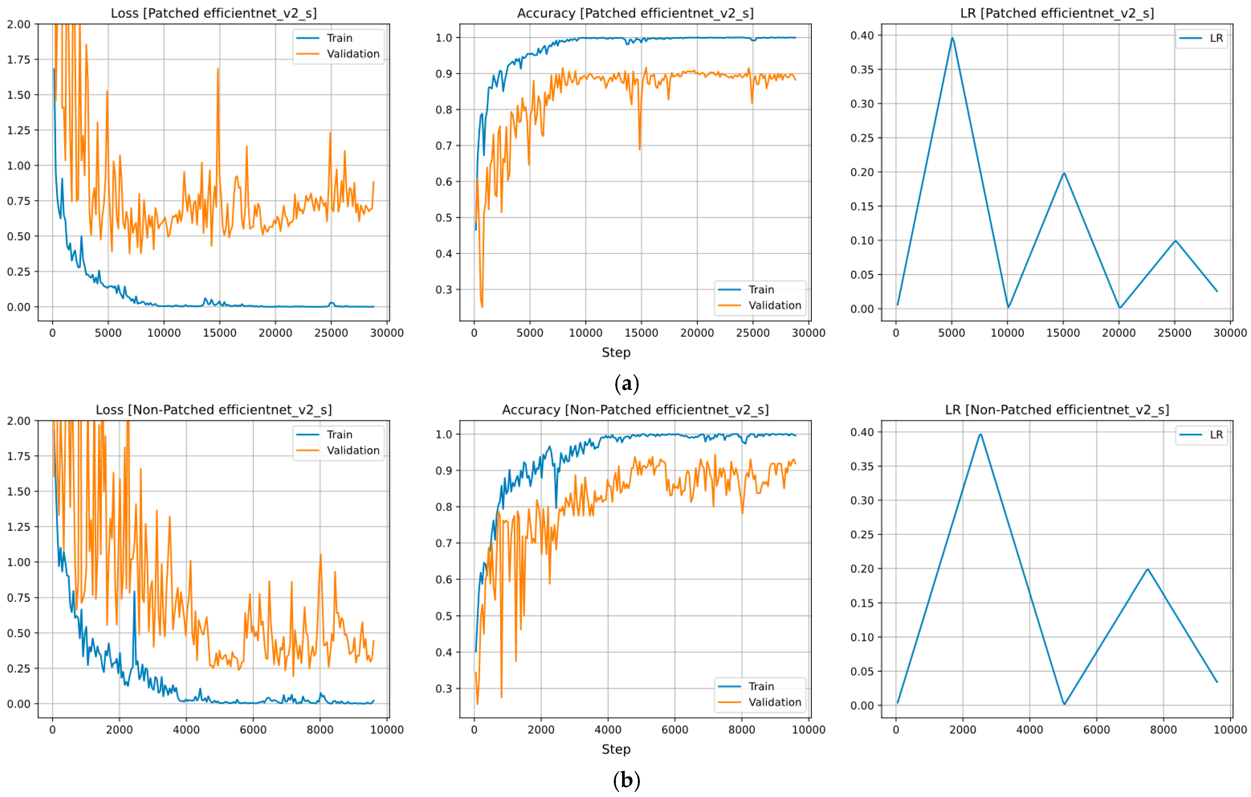
The plots of the loss, accuracy, and learning rate of the patched and unpatched RegNetY800MF model are shown in Figure 4. This variant of the RegNet family performed much better than the rest of its counterparts in terms of test accuracy, precision, recall, and F1-score. Its learning rate scheduler was configured with a base_lr of 10 4 and a max_lr of 0.4; however, since the patched model used twice the batch size of the non-patched model, its cycle size is double that of the non-patched model so as not to rush it into small learning rates and thus slower fitting. The validation accuracy and loss of the patched model experienced fewer oscillations than the non-patched model, but it achieved lower loss and higher accuracy overall.
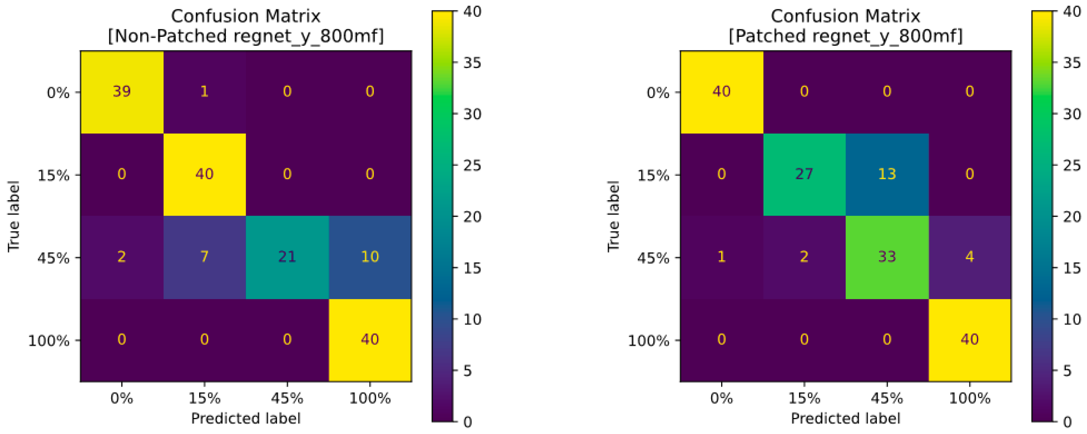
The confusion matrices of the patched and non-patched RegNetY800MF model are shown in Figure 5. The performance measures obtained from the confusion matrix are presented in Table 3. Both models performed well in predicting the 0% and 100% classes correctly; however, they both predicted some 45% samples as 100% incorrectly, which affected their Precision 0 % and Precision 100 % negatively.
For the 15% class, the non-patched model predicted them all correctly, resulting in 100% Recall 15 % . However, it also predicted some 0% and 45% samples as 15%, which affected its Precision 15 % negatively. In contrast, the patched model performed worse for this class, both in terms of its false positives and false negatives, resulting in a poor Recall 15 % . But because its number of true positives was also worse, its Precision 15 % was more than the non-patched model.
For the 45% class, the non-patched model had worse performance in almost every aspect; it had fewer true positives and more false negatives, resulting in a staggering Recall 45 % of 52.5%. But since it had no false positives, it had a perfect Precision 45 % . The patched model had more false positives and true positives while having fewer false negatives, which resulted in a lower Precision 45 % and higher Recall 45 % .
The F1-score can help compare the performance of the models for the 15% and 45% classes in terms of precision–recall tradeoff analysis. Overall, the patched model had a more consistent prediction probability for these classes, while the non-patched model was more likely to predict the 45% class as 15% or 100%.
Overall, the patched model performed slightly better in the case of the F1-score; however, they both had an accuracy of 87.5%.

3.2. Evaluation of MobileNet V3Large Classifier

The loss, accuracy, and learning rate plots of the patched and non-patched MobileNetV3Large model are shown in Figure A1 in Appendix A. Its learning rate scheduler was configured with a base_lr of 2.5 × 10 2 and max_lr of 0.25 ; the reason for the different values for this model was that it did not converge with the usual values for base_lr and max_lr. The validation accuracy and loss of both models experienced a lot of fluctuations, with the non-patched model experiencing more. Even so, the non-patched model achieved higher validation accuracy more frequently than the patched model.
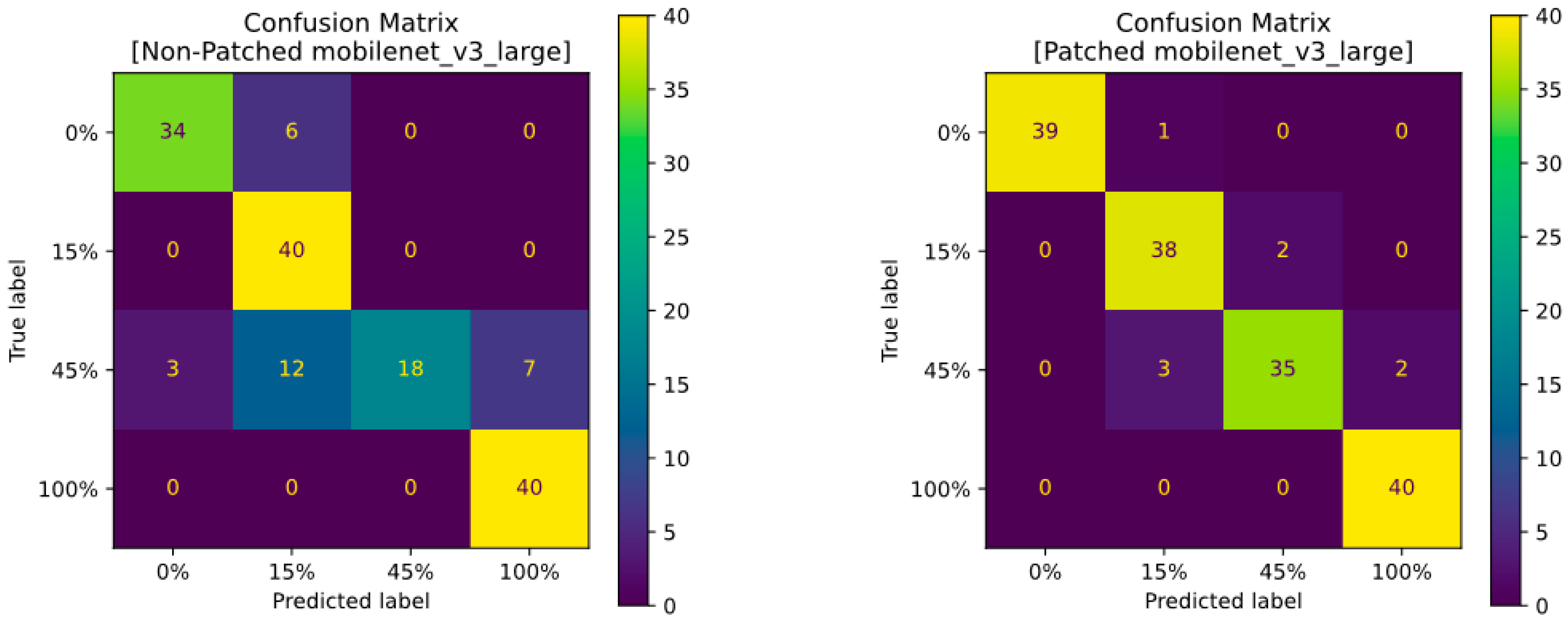
The patched and non-patched MobileNetV3Large models’ confusion matrices are displayed in Figure 6, and the accuracy measures are in Table 4. The patched model performed better in all aspects. The 0%, 15%, and 100% classes almost had no false negatives and slightly more false positives, resulting in high precision and recall. Also, the 45% class had more false negatives, which resulted in a slight decrease in recall compared to other classes. The non-patched model correctly predicted 34 of the 0% class, while the rest were predicted as 15%. However, it classified all 15% samples correctly. This model performed the worst in predicting the 45% samples, resulting in more false negatives, which caused Recall 45 % to suffer. Additionally, due to the absence of false positives for this class, Precision 45 % is 100%. In conclusion, the patched model achieved an accuracy of 95%, while the non-patched model correctly predicted only 87.5% of the samples.

3.3. Evaluation of EfficientNet V2S Classifier

The loss, accuracy, and learning rate plots for the patched and non-patched EfficientNetV2S models are given in Figure A2. Its learning rate scheduler was configured with a base_lr of 10 4 and max_lr of 0.4. Both these models’ validation accuracy experienced some fluctuations, with the non-patched one experiencing more while achieving higher values in general. Also, it bears mentioning that while both models’ validation loss experienced a lot of oscillation, the general trend of the patched model is upward after the 10,000th step (equivalent to the 60th epoch). In contrast, the non-patched model’s validation reached 0.25 multiple times when its learning rate was below 0.05. Therefore, if the non-patched model was continued for another 100 epochs, it could have reached a more satisfactory fitting state.
The patched and non-patched EfficientNetV2S models’ confusion matrices are shown in Figure 7 and Table 5. Among these models, the patched model performed worse and had less accuracy. Both models correctly predicted almost all 0% and 100% samples, resulting in their near-perfect Recall 0 % and Recall 100 % .
The patched model performed the worst while classifying the 45% class, not even predicting half of them right. This resulted in this model’s low Recall 45 % while also affecting the other classes’ precision scores poorly. However, 85% of the 15% class’s samples were predicted correctly, which is acceptable compared to the former class.
The non-patched model performed much better, achieving an accuracy of 90.6% compared to the patched model’s 83.1%. But this model classified about one-quarter of the 45% class samples as 100%, which caused its Precision 100 % and   Recall 45 % to be lower than its other classes. Additionally, this model performed well in the case of the 15% class, predicting 92.5% of them correctly while predicting the others as 0% or 45%. Both models had decent precision–recall tradeoffs, with the non-patched model having about a 10% higher F1-score.

3.4. Evaluation of ShuffleNet V2x10 Classifier

The accuracy, loss, and learning rate plots for the patched and non-patched ShuffleNetV2X10 models are shown in Figure A3. Its learning rate scheduler was configured with a base_lr of 10 4 and max_lr of 0.4. Both models’ validation loss forms an upward concave curve; i.e., they reach a global minimum at around 60 epochs and slowly rise afterward. Additionally, the validation accuracy of the non-patched surpassed 90% but experienced a slight downward trend afterward. Furthermore, the patched model’s validation accuracy was fitted at around 85%. As explained in the following subsection, the patched model’s test accuracy far exceeds that of the non-patched model, likely due to the patched model’s better fit concerning its validation accuracy.
The patched and non-patched ShuffleNetV2X10 models’ confusion matrix is shown in Figure 8, and the performance measures are in Table 6. Similar to previous models, the patched model predicted almost all 0% and 100% samples correctly, with little to no confusion, resulting in near-perfect Recall 0 % ,   Recall 100 % ,   Precision 0 % ,   and Precision 100 % scores. This model also predicted a fair number of the 45% samples correctly while also over-classifying about half of the 15% samples as 45%. This resulted in a high Recall 45 % , low Precision 45 % , and Recall 15 % . Furthermore, the model under-classified the 15% samples, which resulted in a high Precision 15 % . Based on the fact that the 45% class had the lowest precision, it can be deduced that our model is skewed towards predicting samples as this class.
The non-patched model performed astronomically worse than all the others. This model predicted all 100% class’s samples correctly, resulting in its Recall 100 % being 100%; however, since more than half of the 45% samples were also misclassified as 100%, its Precision 100 % was 60.6%. This model also correctly classified nearly 90% of the 15% samples and misclassified the rest as 45% or 100%, resulting in its high Recall 15 % . However, similar to the 100% class, the 15% class also had more false positives than the 45% and 0% classes, which also affected its Precision 15 % negatively, down to less than 60%. On the other hand, unlike the rest of our models, this model’s 0% class had a lot of false negatives, resulting in its less than 60% Recall 0 % . In conclusion, this model was highly skewed towards predicting our samples as either 15% or 100% due to their precision scores being less than all the other classes.
Overall, based on the per-class and average F1-scores of the two models, it can be concluded that the non-patched model had a far worse precision–recall tradeoff, with its Recall 15 % resulting in its low F 1 - score 45 % , ultimately resulting in a lower average F1-score.

3.5. Evaluation of Swin V2T Classifier

The accuracy, loss, and learning rate plots for the patched and non-patched SwinV2T models are shown in Figure A4. Its learning rate scheduler was configured with a base_lr of 2 × 10 7 and max_lr of 8 × 10 4 . Similar to the MobileNetV3Large model, this model diverged with the usual values for base_lr and max_lr. These models’ validation accuracy is almost equal, both becoming fit at around 85%, with a near-90% maximum value. However, the non-patched model had slightly higher test accuracy, which could be because it achieved 90% validation accuracy later during the training process, suggesting a better fit. Both models’ validation loss experienced some fluctuations. Still, when comparing their general trend after becoming fit, the non-patched model’s trend was linear. In contrast, the patched model had a slightly increasing trend, which could be another possible reason for its somewhat lower test accuracy.
The patched and non-patched SwinV2T models’ confusion matrices are shown in Figure 9. The scores presented in Table 7 show that the patched model had slightly higher average precision, recall, and F1-scores, even though its accuracy is 81.2%, while the non-patched model is 85%.
The patched model correctly classified almost all 0%, 15%, and 100% samples, resulting in high recall scores. However, it correctly classified only half of the 45% samples, classifying most of the rest as 100%. This affected its Recall 45 %   and Precision 100 % negatively. Overall, it can be deduced that this model was skewed towards the 100% class.
The non-patched model predicted all 15% samples correctly and even classified some 0% and 45% samples as 15%. This resulted in its perfect Recall 15 % , but it lowered its Precision 15 % down to 75%. In comparison, the model predicted only three-quarters of the 45% samples correctly, misclassifying the rest as 15% and 0%. Additionally, this model correctly predicted less than three-quarters of the 100% samples, classifying the rest primarily as 45%, resulting in a lower Recall 100 % and Precision 45 % .
Overall, the patched model had four more false predictions than its non-patched counterpart, resulting in slightly less accuracy.

3.6. Analysis of Image Size and Resolution

The comparison between the patched and unpatched approaches is useful to analyze the effectiveness of the classifiers as a function of image size and resolution, i.e., the level of detail of the images. While the unpatched approach uses larger images (660 × 440 pixels), the patched approach uses smaller images (440 × 440) but with a higher level of detail, since the original images are not rescaled. However, these two cases are insufficient to draw precise conclusions about the effect of image size and resolution on the classifiers. Therefore, we performed an additional experiment to test other sizes in both approaches.
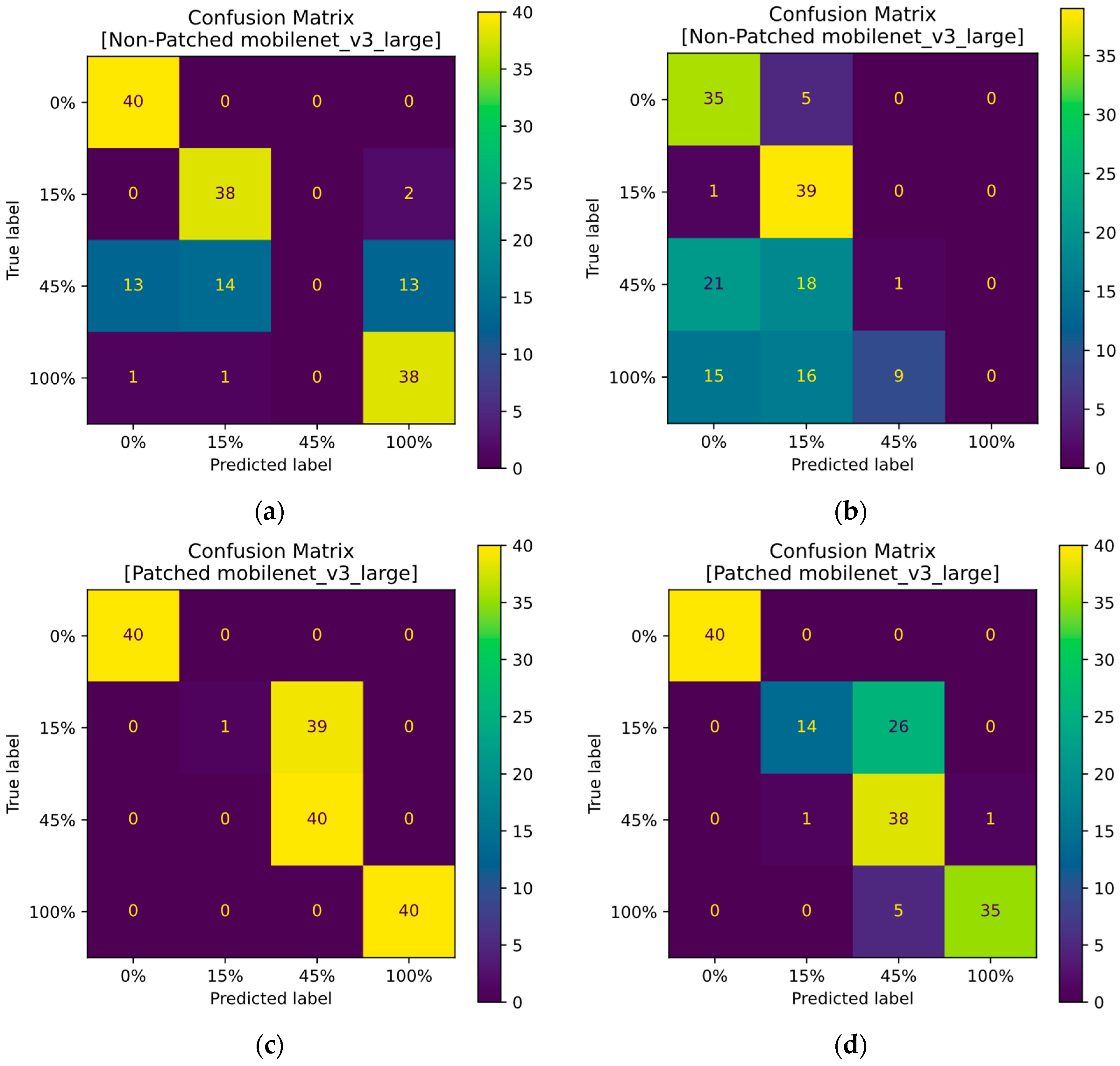
Specifically, in the unpatched version, we tested the use of 330 × 220- (×4 reduction in the original ones) and 160 × 110-pixel images (×8 reduction). In the patched version, the extraction of patches of 220 × 220 (24 patches per original image) and of 110 × 110 pixels (96 patches per image) was tested. For this experiment, only the model that obtained the best overall result in the previous tests was used, i.e., MobileNetV3Large. Although in the unpatched approach, the optimal model was EfficientNet V2S, the MobileNetV3Large network has also been used for it, in order to properly compare the effect of size in both approaches. The classification matrices obtained for each of these variants are shown in Figure 10. Table 8 summarizes the accuracy and efficiency of all of them.
First, the results obtained clearly demonstrate the negative effect of image reduction on classification. The accuracy of the unpatched approach drops from 82.5% for the highest resolution to 72.5% and 46.9% for the reductions by ×4 and ×8, respectively. Training time is also reduced, but in practice, these versions are not feasible. Analyzing why this happens, in Figure 2, we can see that the details that differentiate intact tea from adulterants are very small. By reducing the images ×4 and ×8, these details are lost, so the classifiers are unable to produce a good result. Thus, sufficient resolution is required to see the details of interest in the image.
However, the size of the images is also relevant. Recall that in the patched versions, the images are not resized but divided into small pieces with different sizes. The patched version of 440 × 440 pixels achieved the best accuracy of 95%, compared to the versions of 220 × 220 and 110 × 110 pixels. This worsening occurs even though they have more images for training (which, in turn, translates into longer training times, as shown in Table 8). For example, the 110 × 110 version has 16 times more images than the 440 × 440 version, but its accuracy does not exceed 80%. The reason for these poor results can be seen in the confusion matrices in Figure 10. Although both reduced patched versions achieve the perfect classification of the 0% class, they tend to confuse the classes with 15% and 45% adulterants. In other words, not only is the resolution of the images important in order not to lose details (as we have seen before), but it is also necessary that the images be large enough to make a meaningful sample of the scenes. An image of 110 × 110 pixels only shows about 1% of the original 1320 × 880-pixel image. This small percentage is enough to determine the presence of adulterants, as shown in the confusion matrices, but not to quantify them, producing a great confusion between classes 15% and 45%.

3.7. A Comparison of the Classifiers

Figure 11 and Figure 12 give a comparison of all patched and non-patched models according to the defined evaluation criteria, namely accuracy, precision, recall, and F1-score.
Table 9 compares the correct classification rate (CCR) of the proposed classifiers with other similar works in the current state of the art of visual adulteration detection methods.
As seen in Figure 11 and Figure 12, almost all models achieved scores higher than 80% with the non-patched EfficientNetV2S and patched MobileNetV3Large surpassing 90%. Out of these models, the worst performing model was the non-patched ShuffleNetV2X10 model which seemed to have not been able to find a proper fit, due to its under-classification of the 45% class. Additionally, almost all models achieved a higher precision score compared to their recall score. This is due to the fact that the number of false positives was almost always less than the number of false negatives. As mentioned, the patched MobileNetV3Large model performed much better than the other models—achieving an accuracy of 95% in the best case—which is due to the addition of its new features, namely the Hard-Swish and Squeeze-and-Excitation activation functions which resulted in better nonlinearity and modeling better feature channel interdependencies, respectively.
Furthermore, Table 9 compares our results with several other similar investigations. The most important note to keep in mind is the fact that these papers have different datasets than our own; so, their results cannot be directly compared to our own. However, it can be said that Malyjurek et al. [39] and Kelis et al. [40] used non-CNN methods to analyze hyperspectral images, which resulted in less accuracy. Additionally, Zheng et al. [41] used a symmetric all CNN (SACNN) to analyze hyperspectral images and achieved an accuracy of 92.4%. The usage of hyperspectral images aided in their high accuracy. However, our methods used RGB images, and the patching technique resulted in an accuracy of 95% for the MobileNetV3Large model. The use of standard RGB images has a great advantage over hyperspectral images, since it implies lower camera costs, the greater availability of the cameras, and easier assembly in factories.

4. Conclusions

The development of new techniques for the estimation of the percentage of tea residues in an image is beneficial in the field of agriculture, for example, for the detection of adulteration. In the present work, a new method for adulteration detection in Momtaz tea has been proposed using RGB images and five deep learning models. The problem is posed as a four-class classification problem, where the mixtures range from 100% tea to 100% residue. Two different approaches have been compared, using the whole obtained images and using patches from them. The use of patches is clearly beneficial, as it increases the number of training samples for the models. For the best model, MobileNetV3Large, a classification accuracy of 95% is achieved in the patched approach. This allows for its practical feasibility, recalling that it is a four-class classification problem. The proposed models could be used with other tea varieties and with other types of adulterants. However, this would require obtaining new datasets with which to retrain the models.
As future work, an alternative technique to classification would be to estimate the percentage of tea waste using regression methods. This would allow for an estimate of the degree of adulteration to be given as a percentage of the mixture. However, for this to be possible, it would be necessary to have many more samples and better distributed in the percentages between 0% and 100%. With the available dataset, we did not achieve acceptable results of the models for the regression problem. One possibility is to divide the input images into smaller patches. However, the experiments have shown that in order to achieve good classification accuracy, it is necessary that the images have not only a good level of detail but also a sufficient size to sample the scene to be studied. Another approach is to use some form of an ensemble technique and take a vote between multiple models; this approach can fix the issue of models being biased and over-classifying or under-classifying certain classes. This is due to the fact that some models are better at classifying certain classes, while others over- or under-classify that class. In such cases, the model is said to be biased for or against certain classes. One way to solve this problem would be to use an ensemble of models that all receive the test dataset and take a vote between the models and classify the image as the class that most models classify it as.

Author Contributions

Conceptualization, M.S.B., R.P., S.S., D.S. and G.G.-M.; methodology, S.S.; software, D.S. and M.A.; validation, S.S.; formal analysis, D.S.; investigation, M.S.B., R.P., S.S., D.S., M.A. and G.G.-M.; data curation, R.P.; writing—original draft preparation, R.P.; writing—review and editing, G.G.-M.; supervision, G.G.-M.; project administration, R.P.; funding acquisition, R.P. All authors have read and agreed to the published version of the manuscript.

Funding

This research was funded by project 22130/PI/22 financed by the Region of Murcia (Spain) through the Regional Program for the Promotion of Scientific and Technical Research of Excellence (Action Plan 2022) of the Fundación Séneca-Agencia de Ciencia y Tecnología de la Región de Murcia.

Data Availability Statement

The raw data supporting the conclusions of this article will be made available by the authors on request.

Conflicts of Interest

The authors declare no conflicts of interest.

Appendix A

Figure A1. Loss, accuracy, and learning rate plots of MobileNetV3Large model. (a) Patched and (b) non-patched images.
Horticulturae 10 00665 g0a1aHorticulturae 10 00665 g0a1b
Figure A2. Loss, accuracy, and learning rate plots of EfficientNetV2S model. (a) Patched and (b) non-patched images.
Horticulturae 10 00665 g0a2
Figure A3. Loss, accuracy, and learning rate plots of ShuffleNetV2X10 model. (a) Patched and (b) non-patched images.
Horticulturae 10 00665 g0a3
Figure A4. Loss, accuracy, and learning rate plots of SwinV2 model. (a) Patched and (b) non-patched images.
Horticulturae 10 00665 g0a4

References

  1. Pan, S.-Y.; Nie, Q.; Tai, H.-C.; Song, X.-L.; Tong, Y.-F.; Zhang, L.-J.-F.; Wu, X.-W.; Lin, Z.-H.; Zhang, Y.-Y.; Ye, D.-Y. Tea and tea drinking: China’s outstanding contributions to the mankind. Chin. Med. 2022, 17, 27. [Google Scholar] [CrossRef]
  2. Samanta, S. Potential bioactive components and health promotional benefits of tea (Camellia sinensis). J. Am. Nutr. Assoc. 2022, 41, 65–93. [Google Scholar] [CrossRef]
  3. Samynathan, R.; Thiruvengadam, M.; Nile, S.H.; Shariati, M.A.; Rebezov, M.; Mishra, R.K.; Venkidasamy, B.; Periyasamy, S.; Chung, I.-M.; Pateiro, M. Recent insights on tea metabolites, their biosynthesis and chemo-preventing effects: A review. Crit. Rev. Food Sci. Nutr. 2023, 63, 3130–3149. [Google Scholar] [CrossRef] [PubMed]
  4. Luo, M.; Gan, R.-Y.; Li, B.-Y.; Mao, Q.-Q.; Shang, A.; Xu, X.-Y.; Li, H.-Y.; Li, H.-B. Effects and mechanisms of tea on Parkinson’s disease, Alzheimer’s disease and depression. Food Rev. Int. 2023, 39, 278–306. [Google Scholar] [CrossRef]
  5. Shang, A.; Li, J.; Zhou, D.-D.; Gan, R.-Y.; Li, H.-B. Molecular mechanisms underlying health benefits of tea compounds. Free Radic. Biol. Med. 2021, 172, 181–200. [Google Scholar] [CrossRef]
  6. Ghaderi, Z.; Menhaj, M.; Kavoosi-Kalashami, M.; Sanjari, S. Efficiency analysis of traditional tea farms in Iran. Ekon. Poljopr. 2019, 66, 423–436. [Google Scholar] [CrossRef]
  7. Nasir, N.F.; Mohamad, N.E.; Alitheen, N.B. Fermented Black Tea and Its Relationship with Gut Microbiota and Obesity: A Mini Review. Fermentation 2022, 8, 603. [Google Scholar] [CrossRef]
  8. Balentine, D.A.; Harbowy, M.E.; Graham, H.N. Tea: The plant and its manufacture; chemistry and consumption of the beverage. In Caffeine; CRC Press: Boca Raton, FL, USA, 2019; pp. 35–72. [Google Scholar]
  9. Liang, S.; Granato, D.; Zou, C.; Gao, Y.; Zhu, Y.; Zhang, L.; Yin, J.-F.; Zhou, W.; Xu, Y.-Q. Processing technologies for manufacturing tea beverages: From traditional to advanced hybrid processes. Trends Food Sci. Technol. 2021, 118, 431–446. [Google Scholar] [CrossRef]
  10. Overbosch, P.; Blanchard, S. Principles and systems for quality and food safety management. In Food Safety Management; Elsevier: Amsterdam, The Netherlands, 2023; pp. 497–512. [Google Scholar]
  11. Tibola, C.S.; da Silva, S.A.; Dossa, A.A.; Patrício, D.I. Economically motivated food fraud and adulteration in Brazil: Incidents and alternatives to minimize occurrence. J. Food Sci. 2018, 83, 2028–2038. [Google Scholar] [CrossRef]
  12. Onyeaka, H.; Ukwuru, M.; Anumudu, C.; Anyogu, A. Food fraud in insecure times: Challenges and opportunities for reducing food fraud in Africa. Trends Food Sci. Technol. 2022, 125, 26–32. [Google Scholar] [CrossRef]
  13. Spink, J.W. The current state of food fraud prevention: Overview and requirements to address ‘How to Start?’ and ‘How Much is Enough?’. Curr. Opin. Food Sci. 2019, 27, 130–138. [Google Scholar] [CrossRef]
  14. Wilson, B. Swindled: The Dark History of Food Fraud, from Poisoned Candy to Counterfeit Coffee; Princeton University Press: Princeton, NJ, USA, 2009. [Google Scholar]
  15. Yang, J.; Wang, J.; Lu, G.; Fei, S.; Yan, T.; Zhang, C.; Lu, X.; Yu, Z.; Li, W.; Tang, X. TeaNet: Deep learning on Near-Infrared Spectroscopy (NIR) data for the assurance of tea quality. Comput. Electron. Agric. 2021, 190, 106431. [Google Scholar] [CrossRef]
  16. Zou, Z.; Wu, Q.; Long, T.; Zou, B.; Zhou, M.; Wang, Y.; Liu, B.; Luo, J.; Yin, S.; Zhao, Y. Classification and adulteration of mengding mountain green tea varieties based on fluorescence hyperspectral image method. J. Food Compos. Anal. 2023, 117, 105141. [Google Scholar] [CrossRef]
  17. Li, L.; Cui, Q.; Li, M.; Li, T.; Cao, S.; Dong, S.; Wang, Y.; Dai, Q.; Ning, J. Rapid detection of multiple colorant adulteration in Keemun black tea based on hemp spherical AgNPs-SERS. Food Chem. 2023, 398, 133841. [Google Scholar] [CrossRef]
  18. Dhiman, B.; Singh, M. Molecular detection of cashew husk (Anacardium occidentale) adulteration in market samples of dry tea (Camellia sinensis). Planta Medica 2003, 69, 882–884. [Google Scholar] [PubMed]
  19. Kennedy, S.P.; Gonzales, P.; Roungchun, J. Coffee and tea fraud. In Food Fraud; Elsevier: Amsterdam, The Netherlands, 2021; pp. 139–150. [Google Scholar]
  20. Pal, A.D.; Das, T. Analysis of adulteration in black tea. Int. J. Biol. Res. 2018, 3, 253–257. [Google Scholar]
  21. Pourdarbani, R.; Sabzi, S.; Rohban, M.H.; Garcia-Mateos, G.; Paliwal, J.; Molina-Martinez, J.M. Using metaheuristic algorithms to improve the estimation of acidity in Fuji apples using NIR spectroscopy. Ain Shams Eng. J. 2022, 13, 101776. [Google Scholar] [CrossRef]
  22. Prasetya, A.; Wibowo, N.; Rondonuwu, F. Determination of total quality of black tea fanning grade using near-infrared spectroscopy. J. Phys. Conf. Ser. 2018, 1097, 012008. [Google Scholar] [CrossRef]
  23. Ashqar, B.A.; Abu-Nasser, B.S.; Abu-Naser, S.S. Plant Seedlings Classification Using Deep Learning. Int. J. Acad. Inf. Syst. Res. 2019, 3, 7–14. [Google Scholar]
  24. Xu, W.; Zhao, L.; Li, J.; Shang, S.; Ding, X.; Wang, T. Detection and classification of tea buds based on deep learning. Comput. Electron. Agric. 2022, 192, 106547. [Google Scholar] [CrossRef]
  25. Amsaraj, R.; Mutturi, S. Classification and quantification of multiple adulterants simultaneously in black tea using spectral data coupled with chemometric analysis. J. Food Compos. Anal. 2023, 125, 105715. [Google Scholar] [CrossRef]
  26. Gayathri, S.; Wise, D.J.W.; Shamini, P.B.; Muthukumaran, N. Image analysis and detection of tea leaf disease using deep learning. In Proceedings of the 2020 International Conference on Electronics and Sustainable Communication Systems (ICESC), Coimbatore, India, 2–4 July 2020; pp. 398–403. [Google Scholar]
  27. Hu, G.; Wang, H.; Zhang, Y.; Wan, M. Detection and severity analysis of tea leaf blight based on deep learning. Comput. Electr. Eng. 2021, 90, 107023. [Google Scholar] [CrossRef]
  28. Ding, Y.; Huang, H.; Cui, H.; Wang, X.; Zhao, Y. A Non-Destructive Method for Identification of Tea Plant Cultivars Based on Deep Learning. Forests 2023, 14, 728. [Google Scholar] [CrossRef]
  29. Radosavovic, I.; Kosaraju, R.P.; Girshick, R.; He, K.; Dollár, P. Designing network design spaces. In Proceedings of the IEEE/CVF Conference on Computer Vision and Pattern Recognition, Seattle, WA, USA, 13–19 June 2020; pp. 10428–10436. [Google Scholar]
  30. Andrew, G.; Menglong, Z. Efficient convolutional neural networks for mobile vision applications, mobilenets. arXiv 2017, arXiv:1704.04861. [Google Scholar]
  31. Sandler, M.; Howard, A.; Zhu, M.; Zhmoginov, A.; Chen, L.-C. Mobilenetv2: Inverted residuals and linear bottlenecks. In Proceedings of the IEEE Conference on Computer Vision and Pattern Recognition, Salt Lake City, UT, USA, 18–23 June 2018; pp. 4510–4520. [Google Scholar]
  32. Wang, H.; Qiu, S.; Ye, H.; Liao, X. A Plant Disease Classification Algorithm Based on Attention MobileNet V2. Algorithms 2023, 16, 442. [Google Scholar] [CrossRef]
  33. Tan, M.; Le, Q. Efficientnet: Rethinking model scaling for convolutional neural networks. In Proceedings of the International Conference on Machine Learning, Long Beach, CA, USA, 9–15 June 2019; pp. 6105–6114. [Google Scholar]
  34. Zhang, X.; Zhou, X.; Lin, M.; Sun, J. Shufflenet: An extremely efficient convolutional neural network for mobile devices. In Proceedings of the IEEE Conference on Computer Vision and Pattern Recognition, Salt Lake City, UT, USA, 18–23 June 2018; pp. 6848–6856. [Google Scholar]
  35. Ma, N.; Zhang, X.; Zheng, H.-T.; Sun, J. Shufflenet v2: Practical guidelines for efficient cnn architecture design. In Proceedings of the European Conference on Computer Vision (ECCV), Munich, Germany, 8–14 September 2018; pp. 116–131. [Google Scholar]
  36. Liu, Z.; Hu, H.; Lin, Y.; Yao, Z.; Xie, Z.; Wei, Y.; Ning, J.; Cao, Y.; Zhang, Z.; Dong, L. Swin transformer v2: Scaling up capacity and resolution. In Proceedings of the IEEE/CVF Conference on Computer Vision and Pattern Recognition, New Orleans, LA, USA, 18–24 June 2022; pp. 12009–12019. [Google Scholar]
  37. Liu, Z.; Lin, Y.; Cao, Y.; Hu, H.; Wei, Y.; Zhang, Z.; Lin, S.; Guo, B. Swin transformer: Hierarchical vision transformer using shifted windows. In Proceedings of the IEEE/CVF International Conference on Computer Vision, Montreal, BC, Canada, 11–17 October 2021; pp. 10012–10022. [Google Scholar]
  38. Smith, L.N. Cyclical learning rates for training neural networks. In Proceedings of the 2017 IEEE Winter Conference on Applications of Computer Vision (WACV), Santa Rosa, CA, USA, 25–31 March 2017; pp. 464–472. [Google Scholar]
  39. Małyjurek, Z.; Zawisza, B.; de Beer, D.; Joubert, E.; Walczak, B. Authentication of honeybush and rooibos herbal teas based on their elemental composition. Food Control 2021, 123, 107757. [Google Scholar] [CrossRef]
  40. Cardoso, V.G.K.; Poppi, R.J. Cleaner and faster method to detect adulteration in cassava starch using Raman spectroscopy and one-class support vector machine. Food Control 2021, 125, 107917. [Google Scholar] [CrossRef]
  41. Zheng, L.; Bao, Q.; Weng, S.; Tao, J.; Zhang, D.; Huang, L.; Zhao, J. Determination of adulteration in wheat flour using multi-grained cascade forest-related models coupled with the fusion information of hyperspectral imaging. Spectrochim. Acta Part A Mol. Biomol. Spectrosc. 2022, 270, 120813. [Google Scholar] [CrossRef]
Figure 1. A sample image of the preparation of a tea sample.
Horticulturae 10 00665 g001
Figure 2. Examples of tea samples prepared for the present paper distributed between 4 classes, namely 0%, 15%, 45%, and 100% tea waste.
Horticulturae 10 00665 g002
Figure 3. Comparison of training time, model size (number of parameters), and obtained accuracy for all proposed models.
Horticulturae 10 00665 g003
Figure 4. Loss, accuracy, and learning rate plots of RegNetY800MF model. (a) Patched and (b) non-patched approach.
Horticulturae 10 00665 g004
Figure 5. Confusion matrices of patched and unpatched approach for RegNetY800MF model.
Horticulturae 10 00665 g005
Figure 6. Confusion matrices of the patched and non-patched MobileNetV3Large model.
Horticulturae 10 00665 g006
Figure 7. Confusion matrices of the patched and non-patched EfficientNetV2S model.
Horticulturae 10 00665 g007
Figure 8. Confusion matrices of the patched and non-patched ShuffleNetV2X10 model.
Horticulturae 10 00665 g008
Figure 9. Confusion matrices of the patched and non-patched SwinV2T model.
Horticulturae 10 00665 g009
Figure 10. Confusion matrices of the patched and non-patched EfficientNetV2S model for different sizes and resolutions. (a) Unpatched version, size 330 × 220 pixels; (b) unpatched version, size 160 × 110 pixels; (c) patched version, size 220 × 220 pixels; (d) patched version, size 220 × 220 pixels.
Horticulturae 10 00665 g010
Figure 11. A comparison of the models using the evaluating criteria and the unpatched approach.
Horticulturae 10 00665 g011
Figure 12. A comparison of the models using the evaluating criteria and the patched approach.
Horticulturae 10 00665 g012
Table 1. An example of the values for T P 1 , F P 1 , T N 1 , and F N 1 for a case of 4 classes.
Predicted Label
Class 1Class 2Class 3Class 4
True labelClass 1 T P 1 F N 1
Class 2 F P 1 T N 1
Class 3
Class 4
Table 2. Comparison of training time, model size (number of parameters), and obtained accuracy for proposed models.
Model and ApproachModel Size (MB)Training Time (s)Accuracy (%)
Patched EfficientNetV2S77.57820.06283.13%
Non-patched EfficientNetV2S77.5785.85590.63%
Patched MobileNetV3Large16.1427.60595.00%
Non-patched MobileNetV3Large16.1423.53282.50%
Patched RegNetY800MF21.67211.46587.50%
Non-patched RegNetY800MF21.6723.71187.50%
Patched ShuffleNetV2X104.8604.82185.00%
Non-patched ShuffleNetV2X104.8603.38766.88%
Patched SwinV2T105.62622.94685.00%
Non-patched SwinV2T105.6269.08181.25%
Table 3. The per-class precision, recall, and F1-score of the patched and non-patched approach for the four classes (0%, 15%, 45%, and 100% tea waste) for the RegNetY800MF model.
PrecisionRecallF1-Score
Approach0%15%45%100%Avg0%15%45%100%Avg0%15%45%100%Avg
Patched97.6%93.1%71.7%90.9%88.3%100.0%67.5%82.5%100.0%87.5%98.8%78.3%76.7%95.2%87.3%
Unpatched95.1%83.3%100.0%80.0%89.6%97.5%100.0%52.5%100.0%87.5%96.3%90.9%68.9%88.9%86.2%
Table 4. The per-class precision, recall, and F1-score of the patched and non-patched approach for the four classes (0%, 15%, 45%, and 100% tea waste) for the MobileNetV3Large model.
PrecisionRecallF1-Score
Approach0%15%45%100%Avg0%15%45%100%Avg0%15%45%100%Avg
Patched100.0%90.5%94.6%95.2%95.1%97.5%95.0%87.5%100.0%95.0%98.7%92.7%90.9%97.6%95.0%
Unpatched91.9%69.0%100.0%85.1%86.5%85.0%100.0%45.0%100.0%82.5%88.3%81.6%62.1%92.0%81.0%
Table 5. The per-class precision, recall, and F1-score of the patched and non-patched approach for the four classes (0%, 15%, 45%, and 100% tea waste) for the EfficientNetV2S model.
PrecisionRecallF1-Score
Approach0%15%45%100%Avg0%15%45%100%Avg0%15%45%100%Avg
Patched78.4%87.2%76.0%88.9%82.6%100.0%85.0%47.5%100.0%83.1%87.9%86.1%58.5%94.1%81.6%
Unpatched97.6%92.5%90.6%83.0%90.9%100.0%92.5%72.5%97.5%90.6%98.8%92.5%80.6%89.7%90.4%
Table 6. The per-class precision, recall, and F1-score of the patched and non-patched approach for the four classes (0%, 15%, 45%, and 100% tea waste) for the ShuffleNetV2X10 model.
PrecisionRecallF1-Score
Approach0%15%45%100%Avg0%15%45%100%Avg0%15%45%100%Avg
Patched95.1%91.3%65.5%97.6%87.4%97.5%52.5%90.0%100.0%85.0%96.3%66.7%75.8%98.8%84.4%
Unpatched100.0%58.7%87.5%60.6%76.7%57.5%92.5%17.5%100.0%66.9%73.0%71.8%29.2%75.5%62.4%
Table 7. The per-class precision, recall, and F1-score of the patched and non-patched approach for the four classes (0%, 15%, 45%, and 100% tea waste) for the SwinV2T model.
PrecisionRecallF1-Score
Approach0%15%45%100%Avg0%15%45%100%Avg0%15%45%100%Avg
Patched100.0%86.4%90.9%71.4%87.2%95.0%95.0%50.0%100.0%85.0%97.4%90.5%64.5%83.3%83.9%
Unpatched94.1%69.0%75.0%100.0%84.5%80.0%100.0%75.0%70.0%81.3%86.5%81.6%75.0%82.4%81.4%
Table 8. A comparison of the training time, accuracy, precision, recall, and F1-score achieved by the proposed approaches and image sizes, for the MobileNetV3Large model.
Approach and
Image Size (Pixels)
Training Time (s)AccuracyPrecisionRecallF1-Score
Unpatched 660 × 4403.530.8250.8650.8250.810
Unpatched 330 × 2202.320.7250.5440.7250.621
Unpatched 160 × 1101.940.4690.2720.4690.332
Patched 440 × 4407.610.9500.9510.9500.950
Patched 220 × 2208.020.7570.8770.7560.680
Patched 110 × 11021.980.7940.8640.7940.782
Table 9. A comparison of the correct classification rates (CCRs) achieved by the proposed classification models and other similar works in the literature for adulteration detection using computer vision systems.
AuthorsProductMethodCCR (%)
Present paperTeaRegNetY800MF87.5–87.5
MobileNetV3Large82.5–95.0
EfficientNetV2S90.6–83.1
ShuffleNetV2X1066.9–85
SwinV281.2–85
Malyjurek et al. [39]TeaPartial Least Squares78
Kelis et al. [40]StarchSVM86.9
Zheng et al. [41]FlourCNN92.4
Disclaimer/Publisher’s Note: The statements, opinions and data contained in all publications are solely those of the individual author(s) and contributor(s) and not of MDPI and/or the editor(s). MDPI and/or the editor(s) disclaim responsibility for any injury to people or property resulting from any ideas, methods, instructions or products referred to in the content.