Leveraging Historical Process Data for Recombinant P. pastoris Fermentation Hybrid Deep Modeling and Model Predictive Control Development

Abstract

Hybrid modeling techniques are increasingly important for improving predictive accuracy and control in biomanufacturing, particularly in data-limited conditions. This study develops and experimentally validates a hybrid deep learning model predictive control (MPC) framework for recombinant P. pastoris fed-batch fermentations. Bayesian optimization and grid search techniques were employed to identify the best-performing hybrid model architecture: an LSTM layer with 2 hidden units followed by a fully connected layer with 8 nodes and ReLU activation. This design balanced accuracy (NRMSE 4.93%) and computational efficiency (AICc 998). This architecture was adapted to a new, smaller dataset of bacteriophage Qβ coat protein production using transfer learning, yielding strong predictive performance with low validation (3.53%) and test (5.61%) losses. Finally, the hybrid model was integrated into a novel MPC system and experimentally validated, demonstrating robust real-time substrate feed control in a way that allows it to maintain specific target growth rates. The system achieved predictive accuracies of 6.51% for biomass and 14.65% for product estimation, with an average tracking error of 10.64%. In summary, this work establishes a robust, adaptable, and efficient hybrid modeling framework for MPC in P. pastoris bioprocesses. By integrating automated architecture searching, transfer learning, and MPC, the approach offers a practical and generalizable solution for real-time control and supports scalable digital twin deployment in industrial biotechnology.

1. Introduction

The inherent complexity of biological systems—characterized by interconnected subsystems and nonlinear dynamics—presents enduring challenges for effective bioprocess monitoring and control. Mathematical modeling offers a powerful means to capture and manage this complexity [1]. Over the past few decades, such models have become indispensable in understanding and optimizing bioprocesses, benefiting from advances in computational capabilities and analytical tools. This progress has led to the adoption of advanced modeling approaches, such as genome-scale metabolic models and computational fluid dynamics simulations [2,3]. With the advent of Industry 4.0, modeling has taken on an even more prominent role in the digital transformation of biomanufacturing [4]. However, the limitations of mechanistic models—particularly their reliance on complete system knowledge—have prompted interest in alternative strategies. As a result, machine learning techniques are gaining traction, offering flexible, data-driven alternatives that can extract insights without relying on fully defined system knowledge—supporting next-generation bioprocess digitalization [5,6,7,8].

To bridge this gap, hybrid neural network (HNN) models have emerged as a compelling solution, integrating domain knowledge with data-driven flexibility [9,10,11,12,13,14]. These models combine the structure of mechanistic frameworks (e.g., mass or energy balances) with the flexibility of data-driven components such as ANNs, effectively leveraging both physical laws and empirical data [15,16]. A typical use case involves modeling unknown or complex kinetics using neural networks within a differential equation-based framework. Compared to purely nonparametric models, hybrid approaches often yield more accurate, generalizable, and interpretable results—leading to more robust bioprocess operation and control [17,18]. The recent surge in deep learning methodologies further enhanced hybrid modeling by enabling neural networks to approximate intricate biological functions, as deep neural networks (DNNs) with multiple hidden layers demonstrated superior capacity for learning hierarchical and compositional functions with fewer parameters and reduced sample complexity compared to shallow architectures [9,10,19]. As such, hybrid deep learning models are emerging as powerful tools in the development of digital twins and advanced bioprocess monitoring systems.

However, training deep models requires extensive, high-frequency datasets that are often unavailable in bioprocessing due to high costs, long cultivation times, and sensor limitations [20]. In early-stage bioprocess development or pilot-scale operations, datasets typically only contain a small number of replicates per condition, resulting in limited coverage of the process space and insufficient diversity to support generalizable deep models [21]. Bioprocess data is typically noisy, heterogeneous, and expensive to generate, posing a major bottleneck for training deep architectures. Such data limitations have accelerated the adoption of hybrid modeling frameworks, which leverage both prior process knowledge and empirical data. The promising approach of integrating historical process data through transfer learning frameworks can significantly improve prediction accuracy and reduce the need for extensive new experimental data [22,23].

Gathering experimental bioprocess data is often time-consuming and labor-intensive, limiting the volume of new datasets available for model development. Therefore, leveraging historical data from similar experiments can significantly benefit the development of hybrid process models for new or evolving bioprocesses. Transfer learning (TL) in deep neural networks involves repurposing models trained on a source task to enhance learning on a related target task, particularly when data are scarce. By leveraging pretrained models—often developed on large, generic datasets—TL facilitates improved convergence speed, generalization, and computational efficiency compared to training from scratch [24,25]. In bioprocess engineering, TL enables the adaptation of models trained on well-characterized systems to predict dynamics in novel or data-limited processes. For instance, TL has been successfully applied to model microalgal bioprocess dynamics using limited time-series data, achieving high accuracy in forecasting process behavior [26] and for the quantification and identification of cellular phenotypes from high-content microscopy images [27]. Effective transfer requires the careful selection of source models, layer-freezing strategies, and learning rate tuning to preserve useful features while adapting to the new task [28]. In bioprocess applications, these considerations are critical due to the heterogeneity of biological systems and the frequent lack of large datasets. Nevertheless, TL remains a promising strategy—especially when combined with hybrid modeling approaches that integrate mechanistic insights with data-driven learning [29].

Deep neural network architecture screening typically involves systematic strategies to identify optimal model configurations and hyperparameters. Common methods include grid search, which exhaustively evaluates combinations within a predefined parameter grid [30]. While easy to implement and parallelize, grid search becomes computationally expensive as the number of hyperparameters increases. Random search improves efficiency by sampling configurations at random, often outperforming grid search in high-dimensional spaces where only a few parameters significantly affect performance [30]. A more advanced and efficient approach is Bayesian optimization, which builds a probabilistic surrogate model (e.g., Gaussian Process) to predict performance and selects promising configurations using acquisition functions like Expected Improvement [31]. This strategy significantly reduces the number of required evaluations and is especially valuable when model training is computationally costly. Several studies confirm that Bayesian optimization typically outperforms traditional approaches in terms of sample efficiency and final model performance [30,31].

As the dominant production mode, fed-batch fermentation remains widely used due to its robustness and high product yield, with most biotherapeutics in clinical and commercial use produced using this mode [32,33]. However, maintaining optimal substrate feeding remains a major challenge, requiring precise control to ensure consistent performance. Model predictive control (MPC) has emerged as a powerful strategy to address this, leveraging predictive models to optimize feeding decisions in real time [34,35,36]. Yet, the nonlinear and dynamic nature of high-cell-density fermentations often limits the accuracy of purely mechanistic models, as parameter estimation and unforeseen biological interactions degrade model reliability [37,38]. Hybrid modeling strategies help mitigate these challenges by improving parameter adaptability, accounting for process nonlinearities, and enhancing real-time prediction accuracy [39]. Integrating hybrid bioreactor process models with MPC enhances the optimization and control of bioprocesses, particularly in complex systems like high-cell-density fermentations, resulting in improved modeling accuracy, increased adaptability to changing process conditions, and real-time feedback for increased process stability [40,41,42].

Recent work has explored hybrid modeling in recombinant P. pastoris cultivations, demonstrating performance gains in process control, generalization, and scalability. Ferreira et al. used a serial HNN, consisting of a three-layer feedforward neural network (FFNN) combined with material balance equations, for the dynamic modeling of P. pastoris GS115 expressing scFv in a 50 L pilot bioreactor. This hybrid model was then applied for iterative batch-to-batch control, resulting in a 4-fold increase in the titer after four optimization cycles [12]. However, no network architecture screening was performed, and the model was trained using a fixed configuration without evaluating alternative structures. Pinto et al. revisited the general bioreactor hybrid model and introduced deep learning techniques. Multi-layer networks with varying depths were combined with First Principles equations to form deep hybrid models. Techniques like ADAM, stochastic regularization, and depth-dependent weight initialization were evaluated in this context. The methods were applied to a synthetic E. coli dataset and a 50 L Mut⁺ P. pastoris process, expressing a single-chain antibody fragment. Results showed significant improvements in generalization, with an 18.4% increase in prediction accuracy and a 43.4% reduction in CPU time compared to shallow models [10]. In another study, Pinto et al. developed a hybrid deep modeling method with state-space reduction, applied to a P. pastoris GS115 Mut⁺ strain expressing scFv. Deep FFNNs of varying depths were combined with bioreactor material balance equations and trained using ADAM, semidirect sensitivity equations, and stochastic regularization. A state-space reduction method, based on principal component analysis (PCA) of the cumulative reacted amount, reduced model complexity by 60%, and improved predictive accuracy by 18.5%. Validation with data from nine fed-batch P. pastoris 50 L cultivations highlighted optimization opportunities, with potential increases in an scFv titer of 30% and 80% achieved by optimizing methanol feed and inorganic elements, respectively [9]. Despite these advances, none of the studies addressed transfer learning, nor did they integrate the hybrid models into real-time control architectures. While two studies investigated optimal network architecture selection, none carried out exhaustive design space exploration—such as varying activation functions, layer placement, or layer types—leaving the potential of more performant architectures underexplored.

The present study aims to advance previous work in hybrid modeling of P. pastoris bioprocesses by addressing several key limitations. Specifically, it expands the search for optimal neural network architectures through a systematic screening approach, enabling the identification of robust and efficient model structures tailored to process dynamics. Transfer learning is introduced as a strategy to adapt pretrained hybrid models—originally developed on historical bioprocess data—to a new, much smaller fermentation dataset, thereby reducing the need for extensive retraining while preserving predictive accuracy. Beyond model development, the practical application of the hybrid modeling approach is demonstrated through its integration into an MPC framework. The resulting hybrid MPC system is experimentally validated, showcasing its effectiveness for the real-time optimization and control of recombinant P. pastoris fed-batch fermentations.

2. Materials and Methods

2.1. Experimental Conditions

Cultivations were performed using a recombinant Pichia pastoris X-33 wild-type strain, producing Qβ coat protein VLPs. The construction of the expression vector and the selection of clones for this specific producer are described in detail elsewhere [43].

The batch and feed media formulations were prepared following the “Pichia Fermentation Process Guidelines” provided by the Invitrogen Corporation [44]. Fermentations were carried out in a 5 L bench-top bioreactor (Bioreactors.net, EDF-5.4/BIO-4, Riga, Latvia) with a working volume of 2–4 L. The pH was continuously monitored using a calibrated pH probe (Hamilton, EasyFerm Bio, Bonaduz, Switzerland) and adjusted to 5.0 ± 0.1 with a 28% NH₄OH solution prior to inoculation; it was then maintained at this value throughout the process. Temperature was regulated at 30.0 ± 0.1 °C using a temperature sensor and jacketed vessel control. A thermostatic circulator (LKB Bromma, Multitemp II, Bromma, Sweden) maintained the cooling water at a preset temperature of 6 °C during experiments. Dissolved oxygen (DO) levels were measured using a DO sensor (Hamilton, Oxyferm Bio, Bonaduz, Switzerland) and maintained above 30 ± 5% via a dual cascade strategy, adjusting the stirrer speed between 200 and 1000 RPM (Cascade 1), and supplementing the inlet air with pure O₂ when necessary (Cascade 2). Throughout the fermentation, we sustained a constant airflow or an air/oxygen mixture at 3.0 slpm. A condenser was employed to capture moisture from exhaust gases, and Antifoam 204 (Sigma-Aldrich, Burlington, MA, USA) was added as needed to suppress excessive foam formation. Substrate feeding was controlled with a high-precision peristaltic pump (Longer-Pump, BT100–2J, Baoding, China).

Methanol feeding proceeded in three phases: initially at 0.12 mL·min⁻¹ for 5 h, then at 0.24 mL·min⁻¹ for 2 h, and finally at 0.36 mL·min⁻¹. This continued either until the end of the experiment or for 2–3 h until the hybrid MPC control was activated so that the cells could effectively adapt to methanol utilization.

In experiments where real-time biomass concentration was monitored using an in-situ turbidity probe (Optek-Danulat, ASD19-EB-01, Essen, Germany), the turbidity signal was correlated with biomass concentration using an exponential calibration equation reported previously [45]. To enhance the in-line biomass measurement quality for hybrid model training, an algorithm was implemented to correct for abrupt, anomalous spikes caused by sudden process disturbances. The details of this algorithm are provided in a separate publication [46].

Although the cultivation conditions were generally similar across all historical experiments, some minor differences were present. For detailed information on these variations, as well as the construction of the expression vectors and clone selection, we refer the reader to the original publications [47,48].

2.2. Downstream Processing of Qβ VLPs

Overall, 4.0 g of wet cells was resuspended in 20 mL of lysis buffer (20 mM Tris 8.0, 100 mM NaCl) and disrupted using a French press (4 × 10,000 psi). The suspension was then centrifuged for 30 min at 18,500× g (4 °C). Ammonium sulfate was added to the supernatant to 40% saturation and proteins were precipitated at 4 °C for 60 min. The suspension was then centrifuged for 20 min at 18,500× g (4 °C) and the supernatant was discarded. The precipitate was dissolved in a 20 mM Tris 8.0 buffer and loaded onto the Sepharose 4 Fast Flow size-exclusion column (12 mL volume) in a lysis buffer at 0.3 mL/min. Peak fractions were pooled and loaded onto an anion-exchange Fractogel DEAE (M) column (5 mL volume) in a lysis buffer and eluted with a linear gradient of 20 mM Tris-HCl, 1 M NaCl pH 8.0 at 2 mL/min.

2.3. Analytical Measurements

Cell growth was observed by offline measurements of dry cell weight (DCW), determined gravimetrically. Biomass samples were placed in pre-weighted Eppendorf^® tubes and centrifuged at 15,500× g for 5 min. Afterwards, the supernatant was discarded and the remaining wet cell biomass was weighted. DCW was calculated using a previously determined correlation coefficient.

DCW = WCW × 0.27

(1)

2.4. Dataset for Hybrid Model Training

The characteristics of the dataset of P. pastoris fermentation data used for hybrid model training are compiled in

Table 1. Dataset of P. pastoris fermentations and parameter ranges used for hybrid model training.

Exp No.	Strain, Product	Induction Time, h	DCW, g·L−1	Feed Rate, mL·min−1	Vend, L	Reference
1 *	GS115, HBcAg	65	37.5–101.6	0.12–0.78	2.85	[45,47]
2 *	GS115, HBcAg	45	40.6–113.5	0.12–1.00	3.09
3 *	GS115, HBcAg	43	41.2–120.1	0.12–0.98	3.13
4 *	GS115, HBcAg	50	59.2–120.1	0.12–0.36	2.54
5 *	GS115, HBcAg	51	41.4–96.6	0.12–0.36	2.87
6	GS115, HBcAg	48	49.1–120.0	0.12–0.50	2.88
7	GS115, HBcAg	43	53.7–101.5	0.12–0.36	2.74	Unpublished data
8	GS115, CA IX	54	44.1–84.0	0.12–0.56	2.75
9 *	X-33, LegH	65	55.4–123.2	0.12–0.36	2.57	[48]
10 *	X-33, LegH	46	49.5–95.4	0.12–0.60	2.98
11	X-33, LegH	65	48.9–111.2	0.12–0.36	2.85
12	X-33, LegH	48	56.4–105.3	0.12–0.50	2.63
13	X-33, LegH	50	45.3–101.3	0.12–0.36	2.61
14	X-33, LegH	45	52.9–103.1	0.12–0.36	2.55
15	X-33, LegH	46	45.1–101.3	0.12–0.36	2.52
16	X-33, LegH	65	51.0–101.7	0.12–0.36	2.66
17	X-33, LegH	46	50.6–92.4	0.12–0.60	3.00
18	X-33, Qβ	65	52.5–117.6	0.12–0.49	3.23	This research
19	X-33, Qβ	48	49.3–117.2	0.12–1.00	3.40
20	X-33, Qβ	55	50.1–107.7	0.12–0.36	2.84
21	X-33, Qβ	52	52.9–112.6	0.12–0.87	3.45

* Experiments with real-time turbidity measurements.

.

2.5. Hybrid Process Model Structure and Training

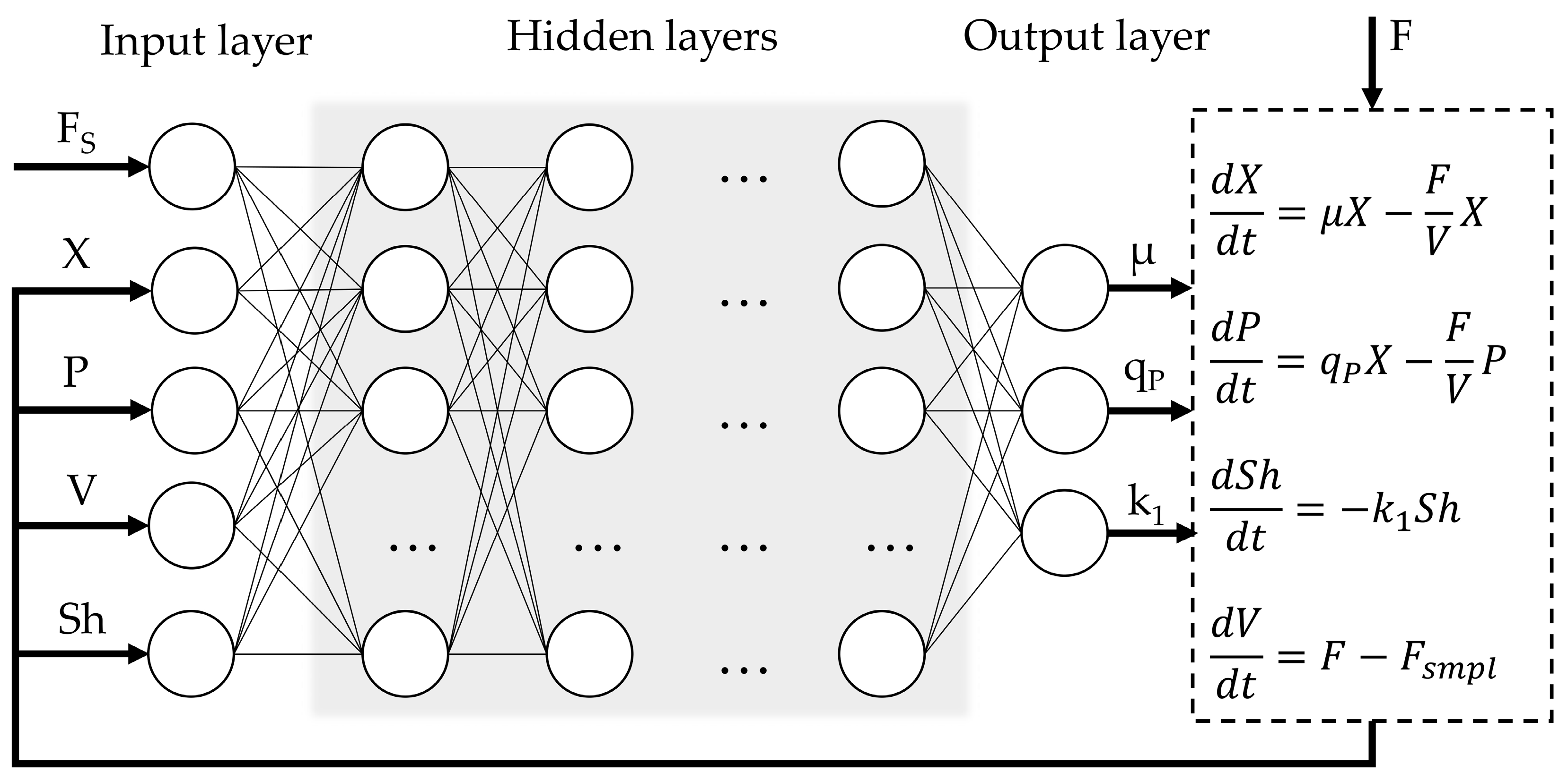
The general structure of the hybrid process model (Figure 1) is similar to the structure previously explored by Pinto et al. [9,10]. The input layer comprises five variables: substrate feed rate (Fs, mL·min⁻¹), dry cell biomass concentration (X, g·L⁻¹), product concentration (P, mg·L⁻¹), culture medium volume (V, L), and an empirical shock factor (Sh). The shock factor equation (Sh(0) = 1) confers the cumulative toxic effect of methanol feeding on the cells and is an unmeasured internal state variable. A similar equation was proposed by Pinto et al. and Lee & Ramirez [9,10,49]. To enhance model training efficiency and convergence, the sequence input layer incorporates the normalization of the input features by scaling each sequence sample to the [0, 1] range using the minimum and maximum values computed over the entire dataset. The output layer provides three variables: the specific cell growth rate (µ, h⁻¹), production rate (q_P, h⁻¹), and the rate of change of the shock factor (k₁). The optimal composition of hidden layer structure was investigated in further steps.

The outputs of the nonparametric model are then passed to the parametric component, which captures the dynamics of the state variables using a system of ordinary differential equations (ODEs) derived from macroscopic and/or intracellular material balances, as well as other relevant physical assumptions. The only external inputs to the model are the aforementioned substrate feed rate (Fs) and the volumetric flow rate (F). This involves the following equation:

$$F=F_s+F_b+F_{AF}-F_{evp}$$

(2)

where F_b and F_AF are the added base and antifoam solution flow rates (mL·min⁻¹) and F_evp is the determined culture evaporation rate (0.11 mL·min⁻¹).

The loss function was defined as the normalized root mean square error (NRMSE):

$$NRMSE={\displaystyle \frac{\sqrt{\frac{{\sum }_{i=1}^n{(y_i-{y_i}^{\mathrm{*}})}^2}{n}}}{y_{max}-y_{min}}}100\%$$

(3)

where n is the number of training samples, y_i represents the measured values, y_i^* is the corresponding predicted variables, and y_min and y_max denote the minimum and maximum values for the dataset, respectively.

To fully utilize the real-time cell biomass sensor data, each process dataset was segmented into 60 equally spaced batches using an interleaved batching approach. Given a time-series dataset consisting of N total time points {t₁, t₂, …, t_N} and a chosen number of segments k = 60, each batch B_j (for j = 1, 2, …, 60) was constructed by selecting every k-th time point starting from offset j. This can be expressed mathematically as follows:

$$B_j=\left\{t_i|i=j+nk, n\in {\mathbb{N}}_0, j+nk\le N\right\}$$

(4)

This approach ensures that each batch contains a temporally distributed subset of the full dataset, preserving temporal variability and aiding in model generalization. For instance, Batch 1 contains {t₁, t₆₁, t₁₂₁, …}, Batch 2 includes {t₂, t₆₂, t₁₂₂, …} and so on, up to Batch 60. Because time-series data were recorded at 1-min intervals, this batching scheme effectively introduced a consistent 60 min gap between successive data points within each batch. As a result, it enabled the estimation of average dynamic rates (e.g., biomass growth or product formation) on an hourly basis—an appropriate timescale for bioprocess interpretation and modeling. This method is particularly suitable for sequence-based machine learning models, as it ensures diverse temporal representation in each training segment.

In experiments where only sparse experimental measurements were available, interpolation was necessary to ensure that each segmented batch contained the corresponding measurement values at the correct time points. To achieve this, piecewise cubic Hermite interpolating polynomial (PCHIP) interpolation was applied to the time-series data. This approach generated estimated values at all necessary time points, thereby ensuring that each batch contained a continuous and temporally consistent signal aligned with the original, sparsely sampled experimental measurements. Importantly, to preserve the integrity of model evaluation, NRMSE was only computed at the original measurement time points, ensuring that model performance was assessed strictly against experimentally observed data rather than interpolated estimates.

Prior to model training, a validation dataset was created by randomly selecting 10% of the original time-series data. Specifically, six batches were sampled from each fermentation experiment to form the validation partition. This subset was held out during training and used exclusively to monitor model performance and assess generalization to unseen data, and as an early-stopping criterion for training.

The hybrid process model was trained using the Adaptive Moment Estimation (ADAM) optimization algorithm, which combines the advantages of both momentum-based and adaptive learning rate methods [50]. The optimizer was configured with standard recommended parameters: the initial learning rate α₀ = 0.001; the first moment decay rate β₁ = 0.9; the second moment decay rate β₂ = 0.999; the small numerical stability constant ε = 10⁻⁸. To facilitate stable convergence and mitigate overfitting, an exponential learning rate decay strategy was employed, where the learning rate was gradually decreased every 100 epochs from 0.001 to 0.0001 by a calculated decay factor over the course of training, as per the following formula:

$$\alpha (t)={\alpha }_0 \ast {\gamma }^{\left[{\displaystyle \frac{t}{100}}\right]}$$

(5)

where α(t) is the learning rate at epoch t and the learning rate decay factor γ = 0.9007.

This gradual decay enabled the model to make larger updates early in training and finer adjustments in later stages, facilitating both rapid convergence and precise parameter tuning. After each epoch, the training dataset was randomly shuffled and divided into six minibatches to support optimization using the ADAM algorithm. This randomization reduced the risk of learning spurious temporal or sequential dependencies and enhanced generalization. The use of minibatches, combined with ADAM’s adaptive learning rate mechanism, further improved training efficiency and convergence reliability.

Hybrid model training was performed using a custom training script developed in the MATLAB environment (MathWorks, R2024b, Natick, MA, USA), leveraging the Deep Learning Toolbox (Scheme S1). Training was conducted on a personal computer equipped with an Intel i5-6600 CPU (3.30–3.90 GHz) and 16 GB of RAM. The training script was parallelized to enable the simultaneous training of multiple networks. For parallel training tasks, the High-Performance Computing (HPC) cluster of Riga Technical University (RTU) was utilized in conjunction with the personal computer. Training for one epoch took approximately 2.5 s.

2.6. Hybrid Model Architecture Screening

To efficiently identify the optimal hidden layer architecture for the hybrid model, a multi-step strategy was implemented. First, a Bayesian optimization approach was employed. This method systematically explores the hyperparameter space by building a probabilistic model of the objective function, enabling informed and efficient searches for the best-performing network configurations with fewer training iterations compared to traditional grid or random search methods.

To accelerate the screening process, networks were trained in parallel for a limited duration of 10 epochs (corresponding to 90 iterations) using an elevated initial learning rate of α₀ = 0.01. This higher learning rate was chosen to promote faster convergence during early training, enabling the quicker identification of promising model architectures without the need for extensive training. Only historical experimental data (Exps. 1–17) was used for hybrid model architecture screening, ensuring the model adapted its parameters based on well-established process dynamics before being fine-tuned with the new Qβ dataset, thereby improving generalization and robustness during transfer learning. Validation loss was used as the primary performance criterion during the grid search, as it provided a more reliable measure of the model’s ability to generalize to unseen data and helped to prevent the selection of overfitted architectures. The corrected Akaike information criterion (AICc) was used alongside validation loss as a performance criterion to account for model complexity, ensuring that selected architectures not only fit the data well but also avoid overparameterization, which can hinder generalization:

$$AICc=n\ln \left(L\right)+2k+{\displaystyle \frac{2k(k+1)}{n-k-1}}$$

(6)

where k is the number of model parameters, L is the loss function value (NRMSE, %), and n is the number of observations (sample size).

For the initial optimization phase, several key hyperparameters were selected to systematically investigate their impact on model performance. These included the choice of the first hidden layer type—either LSTM or fully connected (FC). The number of subsequent fully connected layers was varied between one and two to assess the effect of network depth. Additionally, the activation functions within the fully connected layers were optimized, considering options such as ReLU, Leaky ReLU (0.01), Tanh, or no activation, to evaluate how different nonlinearities affect learning. Finally, the number of hidden units or nodes in each layer was explored within a range of 1 to 5, enabling fine-grained control over model capacity and complexity. This amounts to 8000 possible parameter combinations. The Bayesian optimization algorithm was executed 10 times, each run consisting of 200 iterations. The best-performing model architecture with the lowest validation loss from each run was saved for further evaluation.

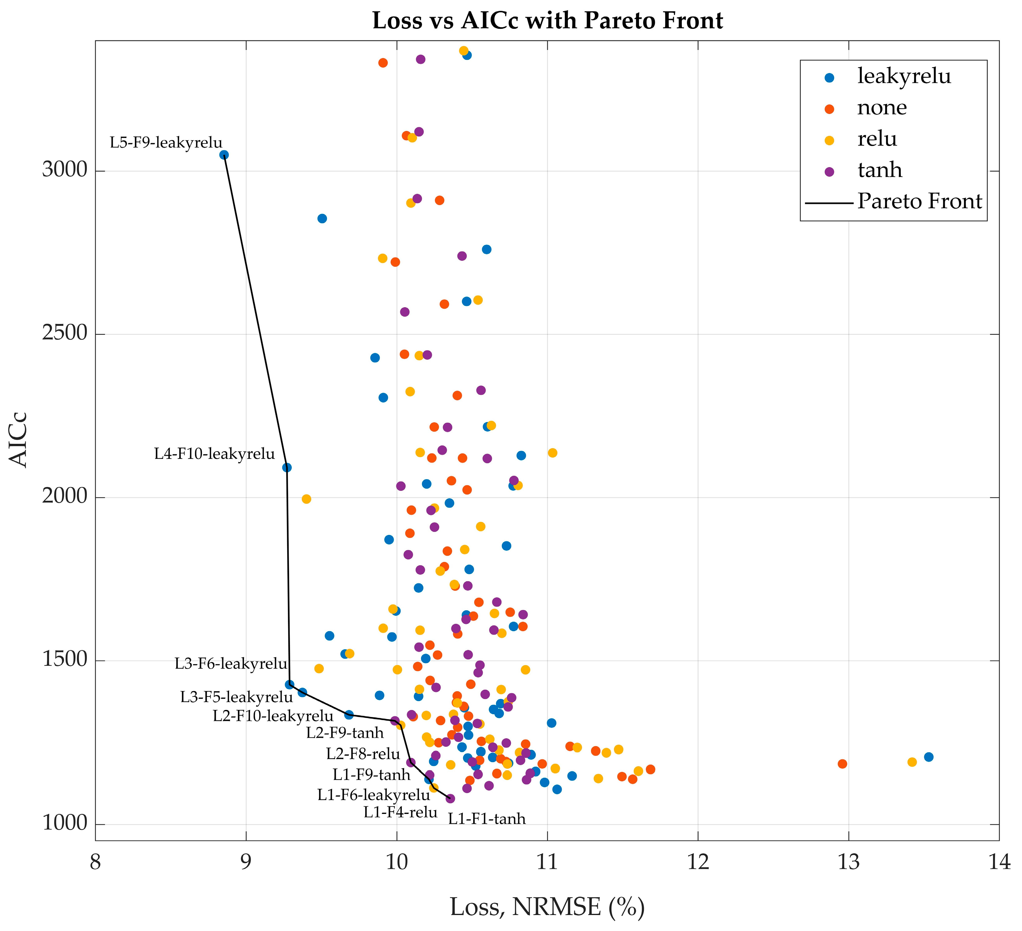
In the second step, the scope of the parameter search was narrowed to focus on the activation function (ReLU, Leaky ReLU, Tanh, or none), the number of LSTM hidden units (ranging from 1 to 5), and the number of fully connected layer nodes (ranging from 1 to 10). The upper limit for LSTM hidden units was intentionally kept low to prevent overparameterization, as each additional LSTM unit substantially increased the total number of trainable parameters. In contrast, the number of FC layer nodes was expanded up to 10 based on favorable results observed in the previous optimization step, where larger FC layers contributed to improved model performance without incurring excessive computational costs. With only 200 possible combinations, a full grid search was conducted during the second screening step. Each network architecture was evaluated across 10 training runs, and only the best-performing candidate was retained for each parameter combination. To balance validation loss with model complexity and mitigate overparameterization, a loss vs. AICc plot was generated to identify the Pareto front (Figure A1). From this front, five network architectures that best balanced low validation loss and favorable AICc values were selected for further evaluation.

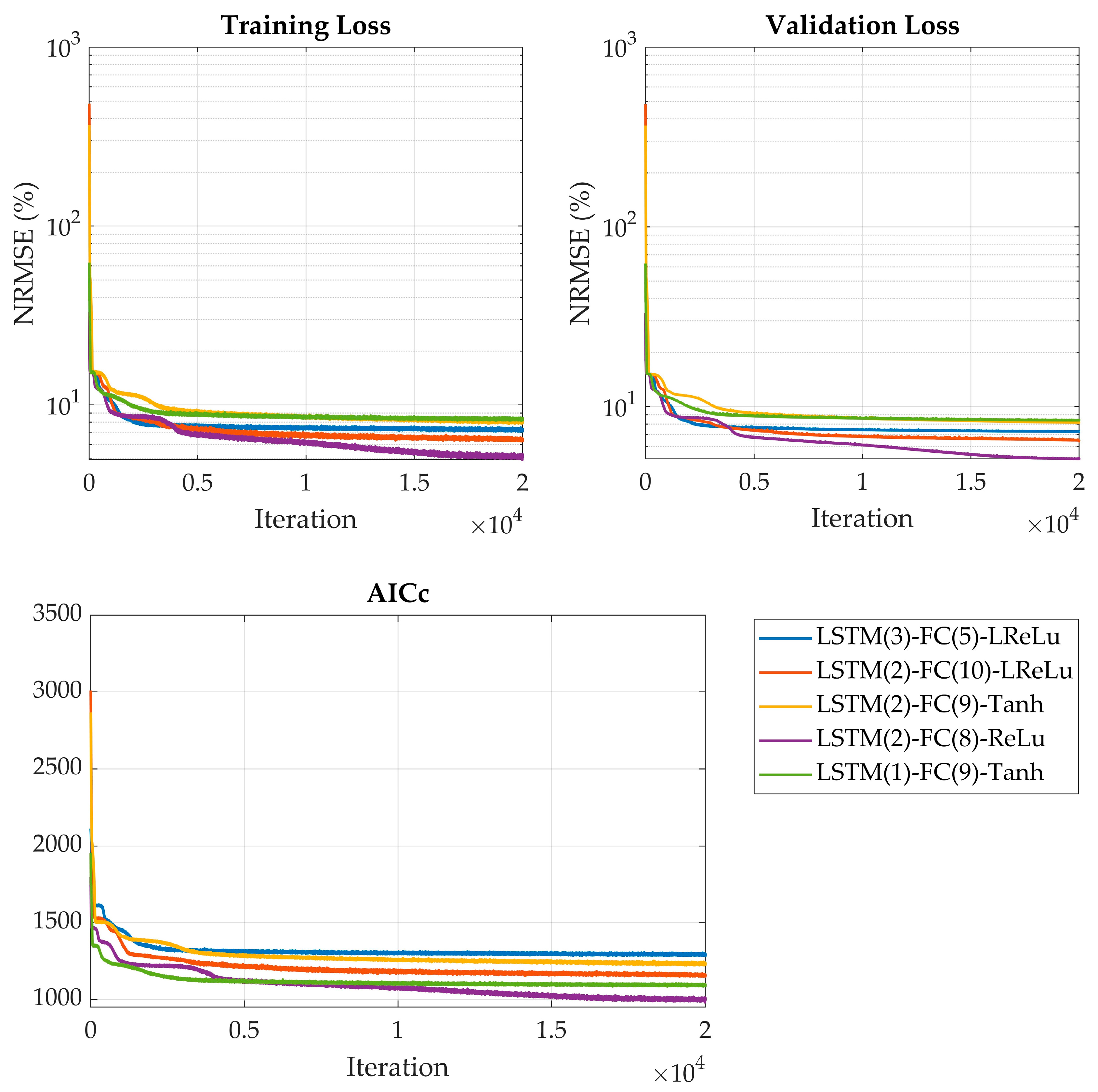
In the third step, the selected models were trained in full for 20,000 iterations, and their predictive performance was assessed using validation loss. The best-performing model was chosen as the optimal network configuration for the specific hybrid process model. Finally, the impact of incorporating a dropout layer within the finalized hybrid model architecture was thoroughly investigated to assess its effect on model robustness and generalization performance.

2.7. Hybrid Model Transfer Learning

To leverage the selected trained hybrid model for a new experimental dataset involving Qβ production, a transfer learning approach was applied. The previously optimized model architecture, trained on the historical dataset, served as the starting point. All model weights were initialized from this pretrained network to retain learned temporal and process dynamics. To adapt the model to the Qβ dataset, only the final fully connected layer was unfrozen and fine-tuned using the new data, while the LSTM unit—capturing general process behavior—was kept fixed. This strategy allows the model to efficiently adapt to the specific characteristics of the Qβ process while preserving useful generalizations from the original training, thereby reducing training time and improving predictive accuracy with limited new data. Experiment 20 was used for testing loss calculation.

2.8. Model Predictive Control (MPC) Architecture

A comprehensive model predictive control framework was developed and implemented, leveraging the advanced hybrid process model. The main task of the MPC controller was to track a pre-selected growth trajectory close to the maximum specific growth rate of the cells.

The MPC algorithm was implemented to dynamically estimate the optimal substrate feed rate, Fₛ(t), required to maintain a desired specific growth rate, μₛₑₜ(t). In the developed hybrid modeling framework, the substrate feed rate served as an input, while the specific growth rate was one of the predicted outputs. Due to the non-invertible structure of the hybrid model, analytical inversion to compute Fₛ(t) from a given μₛₑₜ(t) was not feasible. Consequently, a numerical optimization approach was employed at each control step using MATLAB’s bounded nonlinear optimization function fminbnd, which searched for the optimal feed rate within specified operational constraints. These constraints, set between 0.36 and 1.00 mL min⁻¹, ensured that the substrate feed rate remained within the safe operating range of the bioreactor. The optimization problem at each time step was formulated as follows:

$$\underset{\mathit{Fs}\in \left[0.36, 1.00\right]\mathrm{mL}{\min }^{-1}}{\mathit{min}}{\sum }_{k=1}^{Np}{[\mu \left(k\right)-{\mu }_{set}\left(k\right)]}^2$$

(7)

This was subject to the hybrid model dynamics:

$$x(k+1)=f_{hybrid}(x\left(k\right),F_S\left(k\right))$$

(8)

where x(k) is the vector of the input state variables, and μ(k) is the predicted specific growth rate at step k.

The control horizon was set to N_c = 1 h to match the hybrid model’s prediction timestep, while the prediction horizon was set to N_p = 12 h—twice the estimated dominant time constant of 6 h required for a typical P. pastoris fermentation. The hybrid model itself was simulated with a finer sampling time of 1 min to ensure accurate forward predictions, while the MPC made decisions on an hourly basis.

To improve model accuracy and adaptability, the hybrid model was retrained after each sampling (approx. three times per day). Each time, the newly measured biomass concentration, X_meas(t), was appended to the training dataset, and the model parameters were updated to reflect the latest process dynamics. The pretrained network was fine-tuned for 100 epochs per retraining cycle, requiring on average 5 min per update.

The MPC framework was experimentally validated in a P. pastoris fed-batch fermentation under the methanol-inducible AOX1 promoter. Real-time process data, including substrate feed rate, base and antifoam addition, were integrated into MATLAB via an OPC server, enabling seamless bidirectional communication with the SCADA system. A more technical description is available elsewhere [32]. This real-time data integration allowed the MPC to adjust the substrate feed rate based on actual process conditions.

MPC was initiated after methanol adaptation, typically 8–10 h after induction. The growth rate setpoint μₛₑₜ(t) was scheduled in a step-wise fashion to reflect the physiological limits of the cells: an initial value of 0.04 h⁻¹ was maintained for the first 12 h, followed by reductions to 0.02 h⁻¹ and 0.01 h⁻¹ at 12 h intervals.

3. Results

3.1. Optimal Hybrid Model Architecture Screening

The Bayesian optimization approach was effectively employed to identify optimal hybrid model architectures. Although not all configurations within the design space were explored, the method yielded valuable insights while substantially narrowing the range of candidate architectures. This efficiency stems from the Bayesian framework’s ability to prioritize promising regions of the hyperparameter space, reducing the number of models requiring evaluation. The ten best-performing network architectures, ranked by their validation loss, are summarized in

Table 2. Summary of ten best-performing architectures from Bayesian optimization screening.

First Layer Type	No. of FC Layers	Hidden Units	Nodes	Activation	Validation Loss (%)	No. of Parameters	AICc
LSTM	1	5	5	Tanh	9.73	268	2417
		5	5	LeakyReLu	10.07	268	2431
		5	4	Tanh	10.17	259	2312
		1	5	ReLu	10.26	56	1126
		5	5	Tanh	10.37	268	2444
		3	5	Tanh	10.42	146	1448
		4	5	None	10.51	203	1783
		5	5	Tanh	10.68	268	2457
		4	5	ReLu	10.75	203	1792
		5	4	Tanh	11.30	259	2358

.

The results of the Bayesian optimization screening indicate that while individual performance metrics varied across architectures, consistent structural trends emerged among the top-performing models. Notably, all ten selected architectures include an LSTM layer as the first hidden layer, emphasizing the importance of temporal feature extraction in capturing the dynamics of the process. This is followed in each case by at least one fully connected layer, which likely contributes to nonlinear transformation and the mapping of the LSTM outputs to the target outputs. This consistent architectural pattern suggests that the hybrid model benefits from a sequence-aware representation (via LSTM), followed by flexible function approximation (via FC layers). Although the activation functions and number of units varied, these two structural components formed the core of the most effective configurations, reinforcing their critical role in model performance.

In the subsequent step, a comprehensive grid search was conducted across the full domain of feasible network architectures to investigate the optimal number of hidden units, node counts, and activation functions for the hidden layers. This systematic approach enabled an exhaustive evaluation of all combinations of relevant hyperparameters, ensuring that no potentially optimal configuration within the predefined design space was overlooked. To mitigate the risk of network overparameterization, AICc values were evaluated in parallel with validation loss. Candidate architectures from the Pareto front of the loss vs. AICc plot (Figure A1) were identified as the most promising, and their configurations are detailed in

Table 3. Summary of the best-performing architectures from grid search screening.

Hidden Units	Nodes	Activation	Validation Loss (%)	No. of Parameters	AICc
5	9	LeakyReLu	8.85	304	3050
4	10	LeakyReLu	9.27	243	2092
3	6	LeakyReLu	9.29	153	1427
3 *	5	LeakyReLu	9.37	146	1403
2 *	10	LeakyReLu	9.68	127	1334
2 *	9	Tanh	9.99	121	1316
2 *	8	ReLu	10.03	115	1302
1 *	9	Tanh	10.26	76	1189
1	6	LeakyReLu	10.21	61	1139
1	4	ReLu	10.25	51	1112
1	1	Tanh	10.36	36	1079

* Network architectures selected for the next optimization step.

.

To ensure that there was a balanced trade-off between predictive accuracy and model complexity, the middle five architectures from the Pareto front were selected for further optimization. These architectures, indicated with an asterisk in Table 3, offer a pragmatic compromise: they demonstrate competitive validation losses (ranging from 9.37% to 10.26%) while maintaining a relatively low number of trainable parameters (between 76 and 146). This subset effectively spans the central region of the Pareto front, avoiding both the highly complex models at the top—which, despite slightly better accuracy, incur significantly higher parameter counts and AICc values—and the simplest models at the bottom, which show diminishing returns in terms of validation loss. By focusing on this middle range, the selected architectures are expected to generalize well while remaining computationally efficient and less prone to overfitting.

In the final step, the five selected network architectures underwent an extensive evaluation to rigorously assess their stability and predictive performance. Each architecture was trained independently across 10 separate runs, with each training session lasting for 20,000 iterations. This repeated training procedure helped account for variability due to random initialization and stochastic optimization effects, ensuring the robust comparison of model reliability and convergence behavior. The results, including key performance metrics such as validation loss and generalization capability, from every network’s best session are summarized in

Table 4. Summary of best-performing network architectures.

Hidden Units	Nodes	Activation	Validation Loss (%)	No. of Parameters	AICc
3	5	LeakyReLu	7.28	146	1294
2	10	LeakyReLu	6.37	127	1155
2	9	Tanh	8.14	121	1236
2	8	ReLu	4.93	115	998
1	9	Tanh	8.27	76	1090

, with the training curves shown in Figure 2.

Training results indicate that the optimal network architecture comprises 2 hidden units in the LSTM layer, 8 fully connected layer nodes, and utilizes an ReLU activation function. This configuration achieved the best performance, with a validation loss of 4.93% and the lowest AICc value of 998 among all evaluated models, demonstrating excellent balance between predictive accuracy and model complexity. Among activation functions, ReLU showed significantly better performance than both LeakyReLU and Tanh, aligning with the findings of Pinto et al. [9].

The effects of including a dropout layer with varying probabilities (ranging from 0.1 to 0.5) were systematically evaluated. The results showed that increasing the dropout rate consistently led to higher validation losses. Even a modest dropout probability of 0.1 negatively impacted model performance, suggesting that the selected network architecture is already sufficiently regularized and relatively simple. In such cases, the additional noise introduced by dropout appears to hinder learning rather than mitigate overfitting. This outcome implies that the model generalizes well without further regularization, and applying dropout may introduce unnecessary instability or lead to underfitting. Moreover, the observation may reflect the nature of the dataset, which is likely clean and of limited size—conditions under which every training instance is valuable and even minimal information loss (through activation masking) can reduce training efficiency.

3.2. Adapting the Hybrid Model to Qβ Dataset with Transfer Learning

Finally, the already trained optimal hybrid model was adapted to the new dataset (Qβ fermentations) using transfer learning. The LSTM layer weights were frozen, allowing the network to retain useful generalizations from the original training.

The resulting network demonstrated strong predictive performance, achieving a training loss of 3.18%, a validation loss of 3.53%, and a testing loss of 5.61%. In comparison, the purely historical data-based hybrid model from the previous step, resulted in a testing loss of 11.9% for Exp. 20, showcasing a more than 2-fold increase in predictive power. Together, these metrics indicate that the hybrid model effectively captured the underlying dynamics of the experimental dataset while maintaining generalization to unseen data (Figure 3).

As illustrated in Figure 3, the hybrid model demonstrated strong predictive capability by closely capturing the dynamic behavior of the modeled variables throughout the fermentation process. Quantitatively, the model achieved an NRMSE of 1.68% for biomass concentration (X), indicating high accuracy in cell growth prediction. The product concentration (P), however, was slightly underestimated, resulting in a 9.54% error. Lower product prediction accuracy is to be expected when using such a small dataset, as the whole design space cannot be effectively explored in just 2–3 experiments. Using a larger, more comprehensive experimental dataset would help to improve the recombinant protein concentration prediction accuracy.

3.3. Hybrid MPC Experimental Validation

To evaluate the practical applicability and effectiveness of the hybrid MPC framework, experimental validation was carried out, controlling the feed rate in an actual fermentation run. This allowed for the assessment of the system’s ability to predict and regulate key bioprocess variables in real-time. The results can be seen in Figure 4.

As can be seen in Figure 4, the tracking accuracy of cell biomass (X) by the hybrid model can be characterized as moderate. Notably, the model failed to adequately capture the physiological adaptation phase of P. pastoris to methanol during the first 8–12 h following induction—a period in which cellular growth is minimal or absent. As a result, predictions during this early phase were consistently higher than observed values. However, at the next sampling times (48–51 h), the model accurately predicts the cell biomass concentration, indicating that it does somewhat take into account the reduced growth during methanol adaptation. In the later stages of fermentation, the model exhibited a tendency to overestimate biomass concentration. To compensate for this discrepancy, manual adjustments to the biomass profile were introduced during model retraining, following the availability of offline sampling data. Despite these limitations, the model achieved an overall NRMSE of 6.51% for biomass prediction, indicating acceptable predictive performance.

With respect to product concentration (P), the model similarly demonstrated a tendency to overestimate values across the fermentation timeline. This resulted in an average NRMSE of 14.65%, suggesting moderate accuracy in modeling recombinant protein production dynamics during an actual experimental validation run.

Although the predictive accuracy of the model was not exemplary—particularly in tracking certain state variables with high precision—it nonetheless demonstrated strong performance in its control functionality. Specifically, the model was able to generate robust and reliable feed rate profiles, effectively regulating substrate addition to maintain the desired specific growth rate throughout the fermentation process. This highlights the strength of the hybrid MPC framework in achieving process objectives, even in the presence of moderate prediction errors. The µ tracking results are presented in Figure 5.

As Figure 5 illustrates, the hybrid MPC system demonstrated good performance in tracking the specific growth rate setpoint over the course of the fermentation with a tracking error of 10.64% NRMSE. However, similar to the behavior observed in the prediction model, a slight deviation from the target biomass trajectory was noted during the final 12 h of the process—particularly after the specific growth rate was reduced to 0.001 h⁻¹. This deviation is likely attributable to the cytotoxic effects of methanol accumulation, which can impair cellular metabolism and inhibit biomass formation in the later stages of fermentation. This phenomenon was further reflected in the growth rate tracking plot, where the measured specific growth rate was consistently lower than the target value during this terminal phase. As the purpose of the shock factor is to account for the cytotoxic effects of methanol during the early (adaptation) and late stages of cultivation, revisiting the equation may be warranted.

Overall, while minor discrepancies emerged toward the end of the process, the control system maintained a high degree of accuracy in regulating growth for the majority of the fermentation, underscoring its effectiveness and reliability under realistic bioprocessing conditions.

4. Discussion

This study demonstrates that Bayesian optimization efficiently identifies high-performing hybrid network architectures by focusing on promising hyperparameter regions, reducing the need for exhaustive searches [51]. A consistent architectural pattern emerged among the top models: an LSTM layer followed by one FC layer. This aligns with findings showing that temporal feature extraction via LSTM is critical in sequence modeling, especially in bioprocess contexts [52]. The FC layers then effectively map these temporal representations into nonlinear predictive outputs.

The grid search extended this exploration and employed AICc alongside validation loss to avoid overfitting. The Pareto front strategy is known to balance model complexity and accuracy [30]. Selecting architectures from the midsection of the Pareto front ensured efficient, generalizable models without an unnecessary computational burden. Robustness was confirmed through the repeated training of the selected architectures, mitigating variability from random initialization. The best-performing model—a minimal architecture with 2 LSTM units and 8 FC nodes—achieved the lowest validation loss (4.93%) and AICc (998), illustrating that compact models can deliver strong performance. This has practical implications for real-time applications, where computational efficiency and stability are critical. Interestingly, dropout regularization consistently worsened performance, in contrast to its typical effects in neural networks [53]. This suggests that the additional noise led to underfitting rather than preventing overfitting, corroborating findings in Bayesian LSTM studies [54]. In summary, the combined use of Bayesian optimization and grid search enabled the discovery of robust, efficient hybrid models—providing a practical strategy for developing bioprocess models.

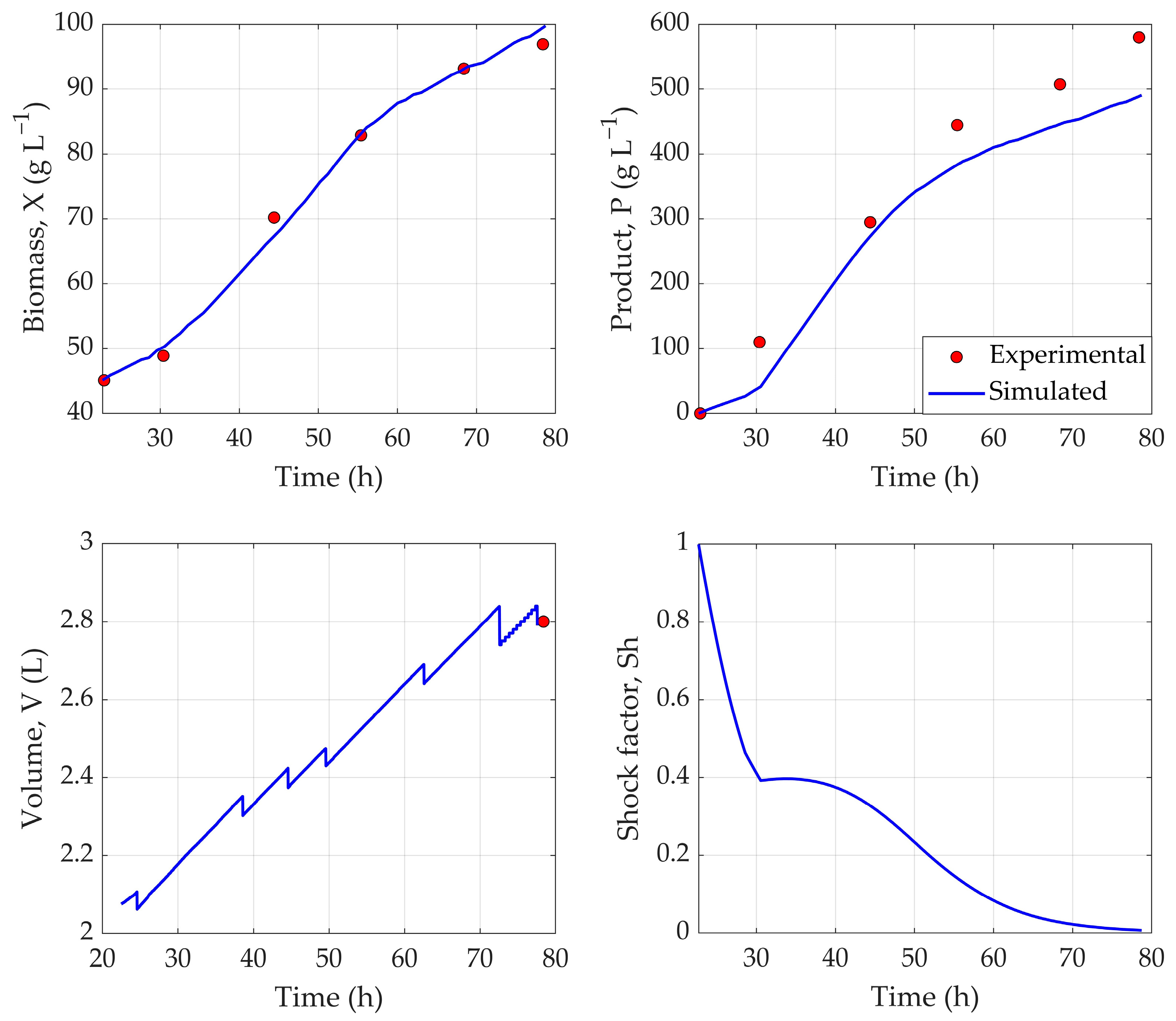
The application of TL showcased its potential for bioprocess applications, as a robust hybrid process model, developed from a historical dataset, was successfully adapted to Qβ fermentations using only three experimental runs. By freezing the pretrained LSTM layer, the model effectively retained temporal feature representations learned from the original fermentation dataset—an approach aligned with the known benefits of sequential inductive transfer learning, where pretrained layers serve as robust feature extractors. Performance metrics indicate a robust predictive capability: a training loss of 3.18%, a validation loss of 3.53%, and a testing loss of 5.61%. 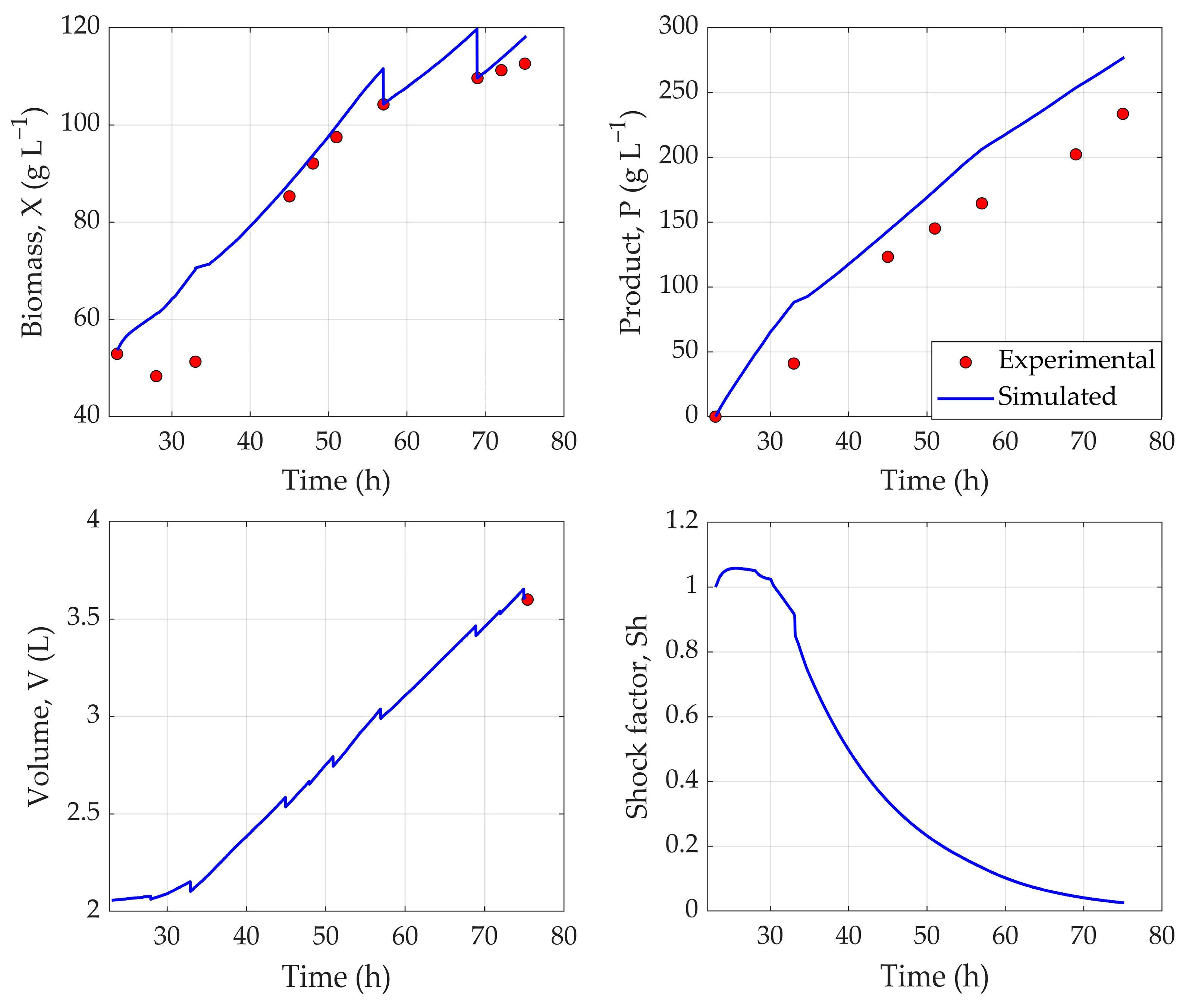Figure 3 illustrates that the hybrid model accurately tracks the dynamic behavior of key process variables throughout fermentation. Notably, the NRMSE of 1.68% for biomass reflects excellent predictive accuracy, while a 9.54% error for product concentration indicates the reliable estimation of recombinant protein output. The performance, especially for product estimation, could further be improved by using a larger experimental dataset that comprehensively presents the fermentation conditions. Overall, the strong performance of the Qβ model—trained on just three fermentations—demonstrates the hybrid model’s generalizability and highlights transfer learning, particularly with LSTM architectures, as a powerful tool for rapid deployment in data-limited fermentation settings [26].

The effective tuning of MPC parameters is essential for achieving stable and responsive control in bioprocesses. In this study, MPC parameters were chosen based on the dynamics of P. pastoris fermentation, informed by operator experience, general rules of thumb, and hybrid model simulations. The typical prediction horizon for P. pastoris fermentations 2–3 times the dominant time constant (τ) is estimated by analyzing the process’s dynamic response—typically from a step change in input. This involves measuring the time it takes the output to reach approximately 63% of its total change. The control horizon is typically 10–20% of the prediction horizon, and in this case is set to 1 h to match the hybrid model’s prediction timestep [55]. In MPC, constraint handling ensures that control actions stay within operational limits, while signal smoothing prevents abrupt changes in control inputs. In this study, the substrate feed rate was constrained between 0.36 and 1.00 mL min⁻¹ to ensure safe operation within the bioreactor’s physical limits, particularly cooling capacity, based on operator experience. These constraints should be tailored for different bioreactor systems and scales. Process simulations with the hybrid model (digital twin) indicated that control signal smoothing was unnecessary, as no abrupt changes in the feed rate occurred. Nevertheless, smoothing should be considered when applying the model to new processes or when operating near the boundaries of the training design space.

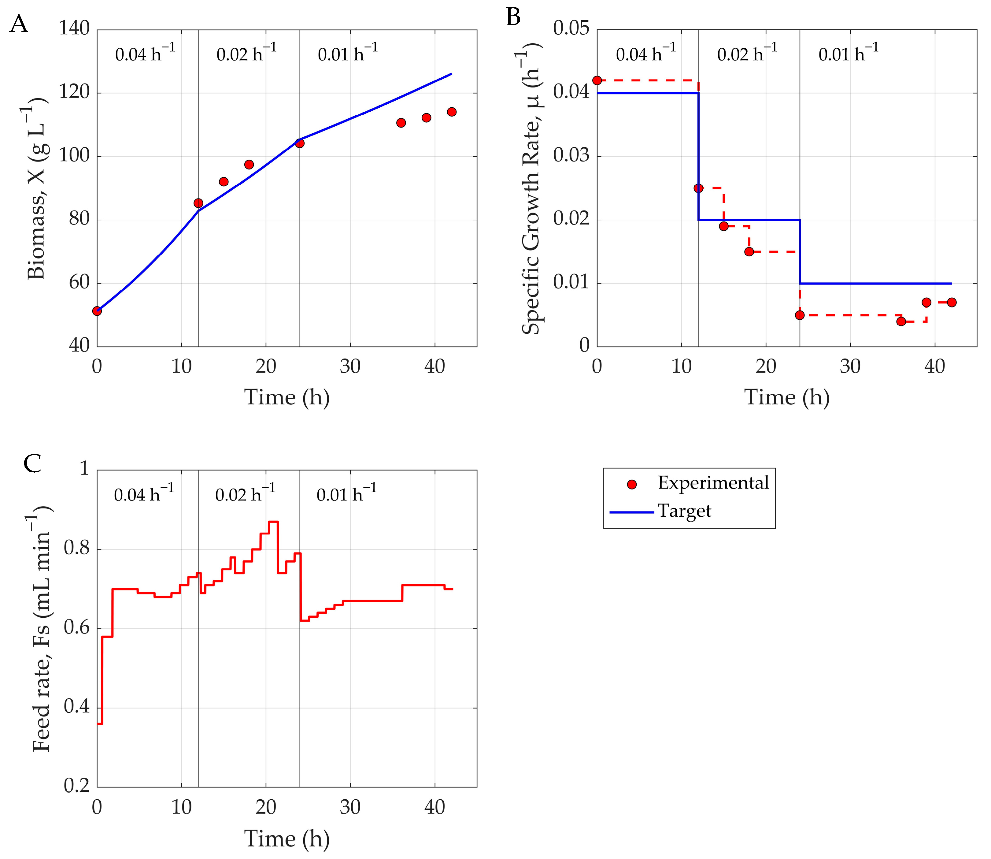
To assess the practical utility of the hybrid MPC framework, a real-time control experiment was conducted, involving feed rate adjustment in an actual P. pastoris fermentation (Figure 4). The hybrid model achieved a biomass NRMSE of 6.51%, indicating moderate prediction accuracy. However, the model struggled during the 8–12 h adaptation phase following methanol induction—likely due to the challenge of capturing initial physiological delays during cell adaptation to methanol uptake. During later stages, persistent biomass overestimation, likely caused by the cumulative cytotoxic effect of methanol, required offline-informed manual corrections. This indicates that the shock factor (Sh) equation should be revisited to better capture the effects of methanol adaptation and cytotoxicity on cell growth. The model also tended to overestimate product concentration, with an average NRMSE of 14.65%, revealing moderate accuracy in tracking recombinant protein dynamics. As previously discussed, this could be addressed with a more comprehensive training dataset. Also, since product concentration cannot be measured at the line, a robust model—such as one based on inputs like biomass (X) or specific growth rate (µ), e.g., the Luedeking–Piret equation—could be used to correct the product inputs during MPC operation to further enhance predictive power.

Despite prediction inaccuracies, the hybrid MPC effectively maintained the target-specific growth rate via robust feed profiles throughout most of the fermentation (Figure 5), with an average tracking error of 10.64%. Only in the final 12 h—particularly after µ dropped to 0.001 h⁻¹—did deviations emerge. These were likely driven by methanol-induced cytotoxicity, which reduced cellular metabolism and hindered biomass formation. The hybrid MPC system showed strong real-time control capabilities, effectively regulating substrate feed to meet specific growth objectives throughout most of the fermentation. Prediction errors were manageable and did not significantly impair overall control performance. This framework can also support tasks beyond growth trajectory tracking—such as production maximization—but would require a more comprehensive dataset to achieve a reliable performance.

This validation confirms that hybrid MPC, built on data-driven hybrid models, is a viable strategy for real-world bioprocess control. Future work should aim to improve model representations of early-stage methanol adaptation, as well as cytotoxicity-induced dynamics towards the end of fermentation. This would further enhance both predictive fidelity and control reliability, supporting broader application in fermentation-based production workflows. Also, a reliable estimator for recombinant protein concentration should be included in the MPC framework to provide accurate and reliable estimations to use for hybrid model retraining during operation.

5. Conclusions

This study presents a comprehensive framework for the hybrid modeling and control of P. pastoris fed-batch fermentations, integrating deep learning with model predictive control. The use of Bayesian optimization proved effective in identifying efficient and accurate hybrid neural network architectures, with consistent structural trends—namely, the inclusion of an LSTM layer followed by fully connected layers—emerging among top-performing models. A grid search guided by AICc and validation loss identified an optimal architecture, balancing accuracy and simplicity. This comprised an LSTM layer with 2 hidden units, followed by a fully connected layer with 8 nodes and ReLU activation. This configuration achieved the best performance, with a validation loss of 4.93% and the lowest AICc of 998.

Transfer learning was successfully used to adapt the hybrid model, originally trained on historical data, to a new Qβ fermentation dataset comprising just three experimental runs. The adapted model maintained strong predictive accuracy (5.61%) while preserving generalizable temporal features. This highlights the model’s flexibility and potential for rapid adaptation to new, yet related, bioprocesses—an important capability in multiproduct biomanufacturing environments.

The experimental validation of the hybrid MPC framework demonstrated reliable real-time control of the fermentation process, despite moderate prediction errors in biomass (6.51%) and product (14.65%) concentration. Notably, the system maintained accurate regulation of the specific growth rate, with an average tracking error of just 10.64% throughout most of the process, deviating only in the final 10–12 h—underscoring its practical robustness.

In summary, this work establishes a robust, adaptable, and computationally efficient hybrid modeling approach for model predictive bioprocess control. The combination of automated architecture search, transfer learning, and MPC provides a scalable methodology for accelerating digital twin deployment in industrial biotechnology.