Comparative Evaluation of Ensemble Machine Learning Models for Methane Production from Anaerobic Digestion

Abstract

This study provides a comparative evaluation of several ensemble model constructions for the prediction of specific methane yield (SMY) from anaerobic digestion. From the authors’ knowledge based on existing research, present knowledge of their prediction accuracy and utilization in anaerobic digestion modeling relative to individual machine learning methods is incomplete. Three input datasets from compiled anaerobic digestion samples using agricultural and forestry lignocellulosic residues from previous studies were used in this study. A total of six individual machine learning methods and five ensemble constructions were evaluated per dataset, whose prediction accuracy was assessed using a robust 10-fold cross-validation in 100 repetitions. Ensemble models outperformed individual methods in one out of three datasets in terms of prediction accuracy. They also produced notably lower coefficients of variation in root-mean-square error (RMSE) than most accurate individual methods (0.031 to 0.393 for dataset A, 0.026 to 0.272 for dataset B, and 0.021 to 0.217 for dataset AB), being much less prone to randomness in the training and test data split. The optimal ensemble constructions generally benefited from the higher number of individual methods included, as well as from their diversity in terms of prediction principles. Since the reporting of prediction accuracy based on final model fitting and the single split-sample approach is highly prone to randomness, the adoption of a cross-validation in multiple repetitions is proposed as a standard in future studies.

1. Introduction

Recent reviews noted that machine learning methods have increasingly demonstrated their ability to capture the complexity of anaerobic digestion processes more effectively than traditional mechanistic models [1,2]. The processing capabilities of large datasets combined with pattern recognition functions allow machine learning to detect sophisticated connections which mechanistic models typically fail to detect. The objective of traditional mechanistic models focuses on describing biological occurrences by using established relationships [3], typically using mathematical formulations that can limit their predictive ability when faced with real-case systems. Machine learning approaches use large datasets to discover statistical correlations, which enables them to refine predictions through observed results instead of using defined operations [4]. Machine learning algorithms succeed in modeling non-linear processes and temporal dynamics because of their ability to adapt to the complex data interactions found in anaerobic systems [5]. The evaluation shows that traditional approaches still have their strengths but demonstrates improvements in methane prediction accuracy through modern machine learning technology [6].

The biochemical methane potential test functions as a vital tool for organic material methane production assessment yet requires improved operational streamlining because its extended testing duration creates barriers to scalable industrial use [7]. Current research interest in predicting methane yield through anaerobic digestion has not received sufficient focus on ensemble machine learning models. Ensemble methods achieve superior predictive performance by uniting individual models to outperform single algorithms in energy production [8,9,10] and smart agriculture [11,12]. Existing research on ensemble approaches for methane yield prediction shows insufficient attention given to defining proper model construction approaches. Existing studies combined evaluation results from all examined non-linear models, yet failed to optimize ensemble selection or architecture [6,13] or selected an arbitrary number of individual methods with the highest prediction accuracy for the ensemble [14]. Failure to optimize ensemble techniques prevents them from reaching their full performance capabilities, resulting in assessments that may not be complete in terms of their individual model performance. The outcome of ensemble machine learning methods depends heavily on the design process, which needs proper attention regarding model combination techniques and diversity management [15]. The analysis performed in past studies disregarded essential elements which could have reduced their ability to measure ensemble model performance and resulted in an inaccurate assessment of predictions for anaerobic digestion methane yield. An optimal design of ensemble methods provides better predictions of methane yield while giving scientists more reliable information about anaerobic digestion, which leads to enhanced decision making in biogas production.

Research on anaerobic digestion modeling with machine learning methods has determined that neural networks along with decision trees, support vector machines, and fuzzy inference systems represent the most commonly used methods due to their high prediction accuracy in predicting methane yield [2,16,17]. The predictive mechanisms of these machine learning techniques vary from one another, which enables them to discover different characteristics of raw data patterns. Artificial neural networks excel at complex non-linear modeling due to their layered structure, yet decision trees boost prediction stability and accuracy by combining numerous decision trees [4]. The regression capabilities of support vector machines reach their best performance in high-dimensional spaces to identify optimal hyperplanes for anaerobic digestion modeling alongside fuzzy inference systems that handle uncertain data patterns commonly observed in laboratory heterogeneity [2]. Ensemble models made up of different methods offer substantial potential for improving robust and accurate methane yield predictions because ensemble approaches balance individual method weaknesses [15]. The combined approach generates better prediction insights than individual modeling methods because it produces reliable results which exceed the accuracy of either method alone for value distribution and input test data properties [13]. A systematic study of ensemble configurations optimized for methane production prediction would produce superior results and insight into the biochemical behavior of anaerobic digestion processes.

The main goal of this study was to evaluate ensemble machine learning model performance for predicting the methane outcome produced by anaerobic digestion through model optimization to achieve superior prediction accuracy. They were evaluated using three datasets consisting of varying input sample and covariate counts to evaluate their robustness alongside prediction accuracy. Existing studies successfully demonstrated single machine learning system functions, but the field lacks systematic assessments of combined methods through ensemble approaches on a laboratory scale.

2. Materials and Methods

Figure 1 presents the comparative evaluation process for ensemble machine learning models which predict specific methane yield (SMY) from anaerobic digestion. This study used three datasets containing diverse numbers of covariates for predicting SMY using previously compiled anaerobic digestion data. An evaluation was conducted on six individual machine learning methods and five ensemble machine learning configurations as part of SMY prediction using 10-fold cross-validation testing across 100 repetitions.

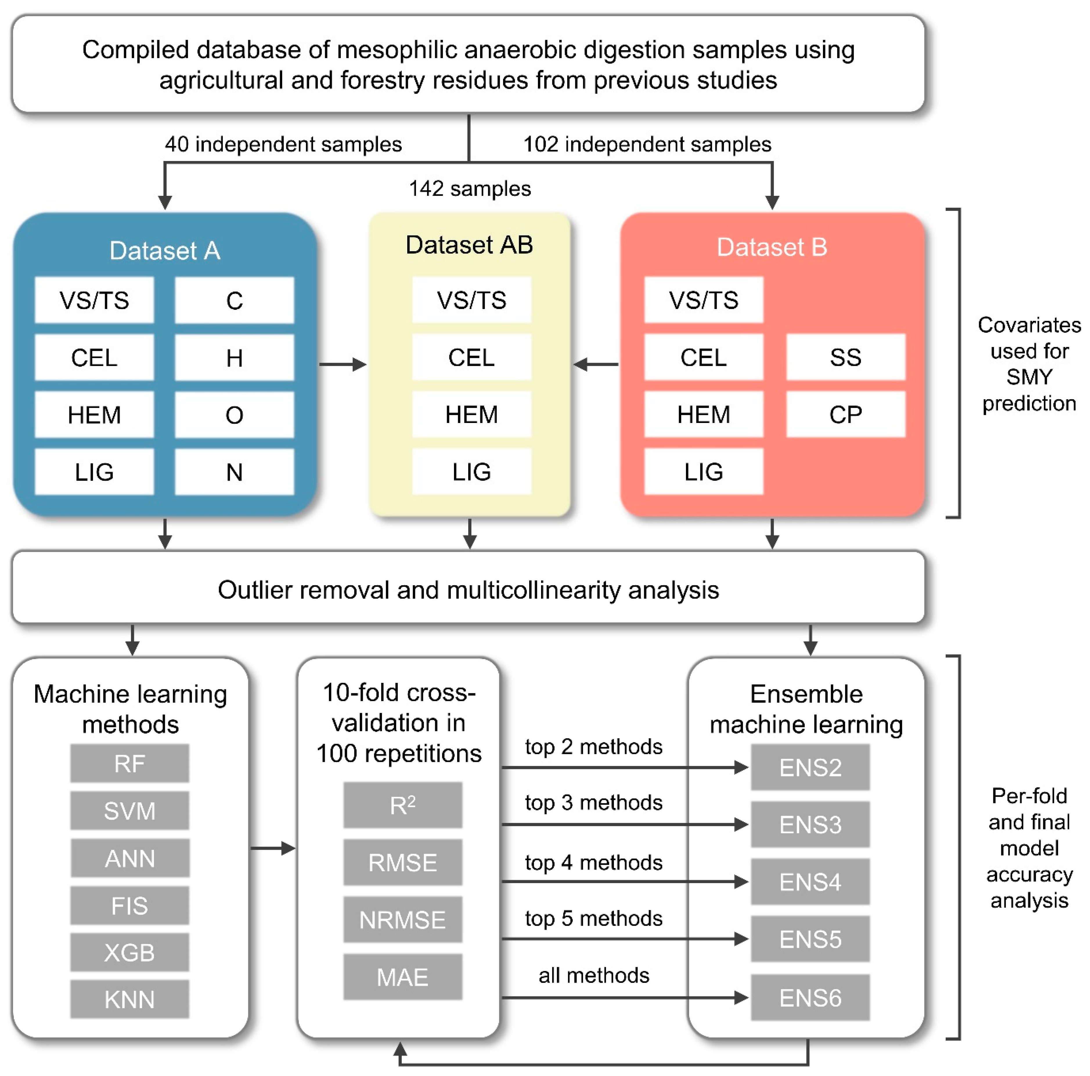
2.1. Input Sample Data Collection and Statistical Preprocessing

The compiled database of mesophilic anaerobic digestion samples using agricultural and forestry lignocellulosic residues from previous studies collected by Wang et al. [6] was used for the comparative assessment of ensemble machine learning. All used samples were based on basic physical pretreatment prior to anaerobic digestion. The initial database consisted of 277 samples, which were filtered to contain only samples based on agricultural and forestry lignocellulosic material, as well as complete data entries which contain all required covariates per dataset. All input samples contained the data on SMY in mL³ g⁻¹ of volatile solids (VS), as well as four covariates, including the ratio of volatile-to-total solids (VS/TS, %), cellulose (CEL, %), hemicellulose (HEM, %), and lignin (LIG, %). However, their remaining covariates consisted of either elemental compositions including C (%), H (%), O (%), and N (%) or soluble saccharide (SS, %), and crude protein (CP, %). To utilize the initial compiled database as much as possible, three datasets were created and used for the comparative assessment of ensemble machine learning for SMY prediction. Datasets A and B were created from mutually independent samples, with dataset A consisting of 40 samples and dataset B consisting of 102 samples. Samples in dataset A had eight covariates (VS/TS, CEL, HEM, LIG, C, H, O, N), while dataset B had samples with six covariates each (VS/TS, CEL, HEM, LIG, SS, CP). Finally, a comprehensive dataset AB was created by merging datasets A and B and retaining covariates which were available for all samples in the dataset, including VS/TS, CEL, HEM, and LIG. The creation of three datasets enabled the evaluation of ensemble machine learning constructions for SMY prediction under various sample and covariate count scenarios to test the relationship between input data properties and model performance. Spearman’s correlation coefficients were used to assess the degree of correlation between SMY and covariates for each of the three datasets. This approach produced three datasets which were mutually different in terms of sample quantity and focused on chemical components and elemental compositions of lignocellulosic material, allowing robust assessment of the ability of ensemble machine learning to predict SMY and evaluate its accuracy relative to the properties of the input dataset.

2.2. Comparative Evaluation Process of Ensemble Machine Learning Models for Predicting SMY

2.2.1. Ensemble Construction Process and Input Data Preprocessing

The individual machine learning methods covered a variety of core machine learning prediction principles to improve the ensemble approach, which generally benefits from diverse methods [15,18]. These core machine learning types consisted of representative algorithms for neural networks, decision trees, support vector machines, fuzzy inference systems, and instance-based learning, which achieved high prediction accuracy in previous studies [2,6,16,17]. A total of six individual machine learning methods were chosen for evaluation according to these criteria, including random forest (RF), support vector regression (SVM), artificial neural networks (ANNs), hybrid fuzzy inference systems (HYFISs), extreme gradient boosting (XGB), and k-nearest neighbors (KNN). In addition to evaluating the prediction accuracy of six individual machine learning methods for SMY prediction, five ensemble approaches were constructed and evaluated for each dataset based on the relative prediction accuracy of individual machine learning methods.

The ENS2 models combined the two most accurate individual models per dataset, while ENS3 and ENS4 integrated the three and four models with the highest prediction accuracy, respectively, and ENS5 aggregated all five individual machine learning methods. This produced a total of 11 models per dataset, allowing a comprehensive evaluation of the optimal ensemble machine learning construction relative to individual methods. All input data were normalized prior to training the machine learning models using a min–max approach. The outlier detection and removal were performed using an interquartile approach, with the threshold of 1.5 times the interquartile range for all three datasets. All predictions were performed using R v4.3.2 [19] with “caret” [20] and “caretEnsemble” [21] libraries. The hyperparameters were tuned for each model based on a random search approach in 10 repetitions, generating a set of random hyperparameters and selecting the most accurate combination based on a 10-fold cross-validation.

2.2.2. Individual Machine Learning Methods Used for Constructing Ensemble Models

The detailed data on R libraries used for individual machine learning predictions and their tuning hyperparameters are presented in

Table 1. Six individual machine learning methods used for ensemble model construction for SMY prediction.

Machine Learning Type	Machine Learning Algorithm	Abbreviation	Tuning Hyperparameters	R Library	Reference
Decision trees	Random forest	RF	mtry, splitrule, min.node.size	ranger	[22]
Support vector machines	Support vector regression with radial basis function kernel	SVM	sigma, C	kernlab	[23]
Neural networks	Artificial neural network	ANN	size, decay	nnet	[24]
Fuzzy inference system	Hybrid fuzzy inference system	FIS	num.labels, max.iter	frbs	[25]
Decision trees	Extreme gradient boosting	XGB	nrounds, max_depth, eta, gamma, colsample_bytree, min_child_weight, subsample	xgboost	[26]
Instance-based learning	K-nearest neighbors	KNN	k	base R	[19]

.

RF constructed a multitude of decision trees during training and outputted their mean prediction, employing bootstrap aggregated with random feature selection, which helps reduce overfitting and improve generalization [27]. At each node of the tree, a subset of features was randomly chosen, and the best split was determined based on the Gini impurity. This randomness in both data sampling and feature selection ensured that the trees are diverse, leading to a more stable and accurate model. RF does not require extensive parameter tuning, and their ability to handle large datasets with high dimensionality makes them particularly suitable for complex datasets, where multiple variables interact in complex ways [16]. XGB, as another method based on decision trees, operated on the principle of boosting, which involved combining the predictions of multiple weak learners to create a strong predictive model [28]. The process built trees one after another in sequence while each subsequent tree intended to address errors present in the preceding ones. Training started from the mean value prediction before moving to additional trees, which refined predictive errors from previous trees through minimizing loss functions. XGB adopted both L1 and L2 regularization to preserve accurate predictions while controlling model complexity according to [29].

SVM computed an optimal hyperplane to fit the data, which accepted errors up to specific tolerance boundaries to determine the ideal linear boundary while allowing some error with no associated cost [30]. The training process needed to detect support vectors which corresponded to the data points that were closest to the hyperplane. SVM utilized a loss function that passed over all errors below designated margins which granted resistance to outliers in the data. SVM adopted the radial basis function as a kernel to expand its capability in analyzing complex patterns beyond simple linear models. The radial basis function kernel enabled complex pattern recognition in datasets due to its adaptive nature, which controlled support vector influence [31].

ANNs are computational models inspired by the biological neural networks that make up animal brains, consisting of interconnected layers of nodes, or neurons, where each connection had an associated weight [32]. The input layer collected information which went through one or multiple hidden layers until an output was generated. The neurons in the network used a non-linear function on their inputs to reveal hidden data relationships. The training phase for the ANN required using optimization algorithms such as backpropagation and gradient descent to adjust weights because it minimized the prediction errors compared to the actual results. Through constant training, the ANN became proficient at recognizing complex non-linear patterns and thus became an ideal tool for predicting methane yield from anaerobic digestion because the relationships between digestion parameters and methane output were very complex and non-linear [2,4].

FIS combined the principles of fuzzy logic with the adaptive learning capabilities of neural networks, allowing it to effectively model complex, non-linear relationships in data while maintaining interpretability through linguistic rules [33]. The structure of hybrid FIS required both data-based fuzzy rule creation and neural network methods to optimize these rules. To begin the process, the system constructed fuzzy rules from data pairs that converted input data into fuzzy values for membership function processing [2]. Utilizing error backpropagation, which is a typically used neural network method, refined the fuzzy rule parameters to achieve better accuracy and adaptability during the second stage. The multilayer structure of FIS includes five separate levels in its design. The initial layer implemented fuzzification to transform crisp input data into fuzzy values through member functions that were pre-established. The system determined firing strengths through its subsequent layers before it normalized those strengths to generate output values which combined weighted rule contributions.

KNN calculated predictions according to the similarity between data points based on k-nearest neighbors to a given point according to the Euclidean distance to quantify the closeness of data points [34]. The prediction value for a given point relied on an average of target values from k-nearest neighbors. Weighted average computations became necessary to determine the final prediction by providing a higher influence on adjacent data points compared to distant ones. KNN regression stands out for its ability to process diverse data distributions because it avoids requirements for specifying any intrinsic structural properties. KNN experiences problems when analyzing data with many dimensions [35] since the dimensionality curse leads to performance degradation and higher computational expenses.

2.3. Accuracy Assessment of Predicted SMY Values

A 10-fold cross-validation in 100 repetitions was employed for accuracy assessment of all individual and ensemble machine learning models in this study. Four statistical metrics were applied, including the coefficient of determination (R²), root-mean-square error (RMSE), normalized root-mean-square error (NRMSE), and mean absolute error (MAE). Model effectiveness assessments were possible through RMSE which measured the average prediction error size but remained sensitive to larger residuals, whereas NRMSE normalized the residual mean square error by dividing it with the mean of SMY values, allowing dataset and model comparison. MAE provides an average measurement of absolute errors which function independently of their direction and remain stable against outliers [36]. Performance evaluation of the models became possible through a complete framework using R² for explained variance measurement alongside RMSE and MAE for absolute accuracy assessment. The normalized property of NRMSE allowed predictive accuracy comparisons between the three datasets effectively. These metrics were frequently used in similar previous studies, thus allowing a comparison with the prediction accuracy results from this study [2]. The increased R² along with decreased values of RMSE, NRMSE, and MAE indicate superior prediction precision.

3. Results and Discussion

3.1. Correlation Analysis of Three Datasets Used for SMY Prediction

Covariates across all three datasets exhibited low to moderate Spearman’s correlation coefficients with SMY, with VS/TS exhibiting the highest absolute value for dataset A, while LIG showed the highest absolute value for datasets B and AB (Figure 2). Overall, there was a difference in the relationship between SMY and the chemical components of lignocellulosic material across the three used datasets. Most notably, CEL had a weak negative correlation with SMY in datasets A and AB, and a weak positive correlation with SMY in dataset B. HEM a showed positive correlation with SMY in all three datasets, with a relatively high range of Spearman’s correlation coefficients of 0.04–0.29. A similar observation was made for the correlation between SMY and LIG, which ranged from −0.25 in dataset A to −0.66 in dataset AB. Besides the notable heterogeneity between input values from the three datasets used in this study, their properties were slightly different from previous, similar studies. Sonwai et al. [37] used a similar approach of compiling an input dataset with samples from previous studies with 205 total samples, which produced a comparable correlation between SMY and HEM (0.15), while LIG (−0.25) and CEL (0.14) were on the higher end of the value ranges from this study. Additionally, the correlation between SMY and C (0.20) from that study was very comparable to dataset A, while their data on N (0.24) produced notably different properties in comparison to dataset A from this study, which had a negative correlation with SMY. In another study by Song et al. [38], which was based on mostly agricultural waste, the cumulative methane yield produced a comparable correlation to this study for VS/TS (−0.04), LIG (−0.43), and H (0.05), while its relationship with HEM (−0.04), CEL (0.28), C (−0.10), N (−0.02), and O (−0.13) did not correspond to those from datasets in this study. While it is well documented in the literature that SMY generally has a moderately high negative correlation with LIG and a low positive correlation with HEM [6], the remaining relationships are highly subjected to the type of substrates for anaerobic digestion [39], available covariates [40], and the number of input training samples [41]. Therefore, the evaluation of machine learning models on multiple input datasets could significantly improve the robustness and reliability of their prediction accuracy under various conditions, which is currently one of the main challenges in translating these models from laboratory- to industrial-scale production [17].

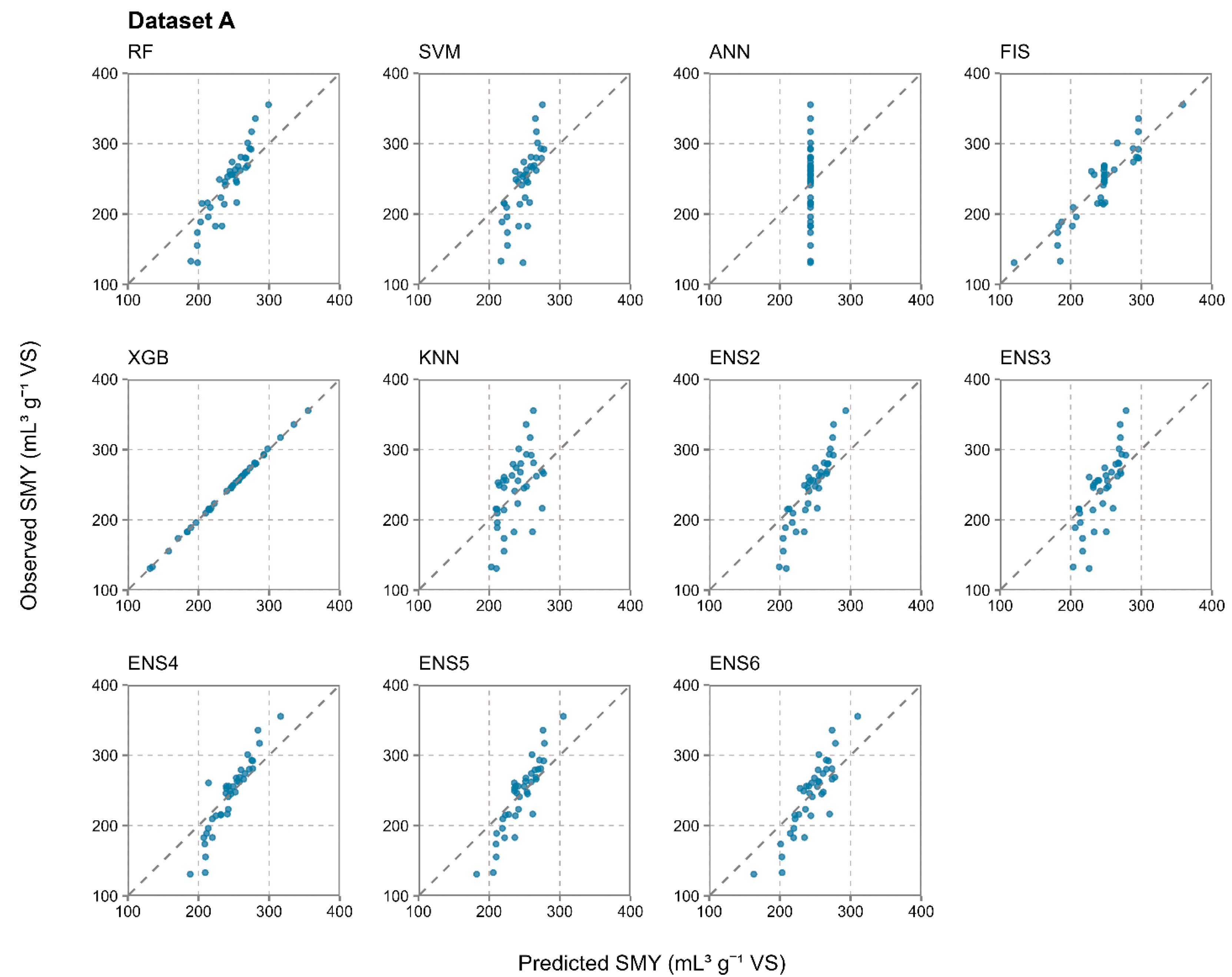
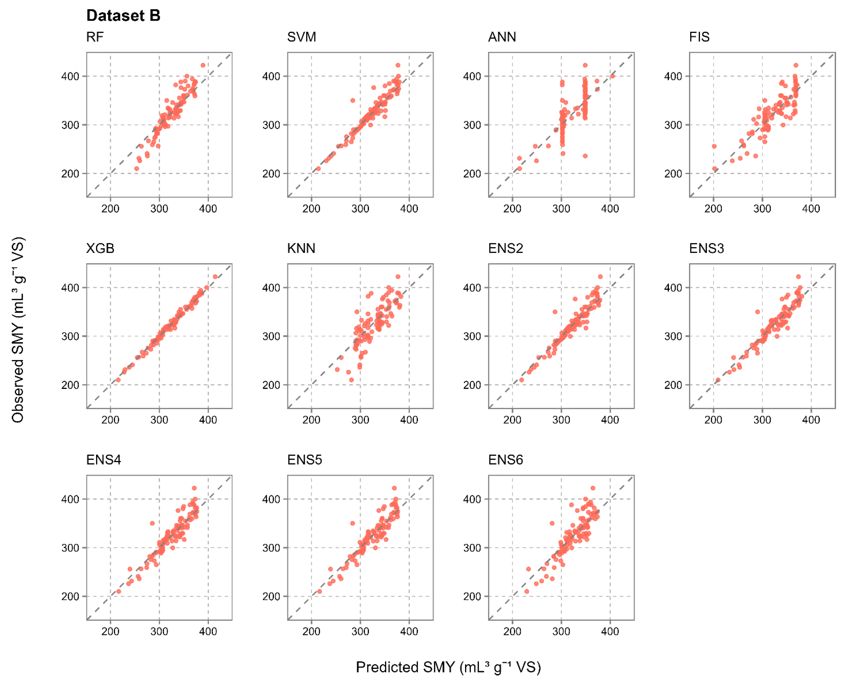
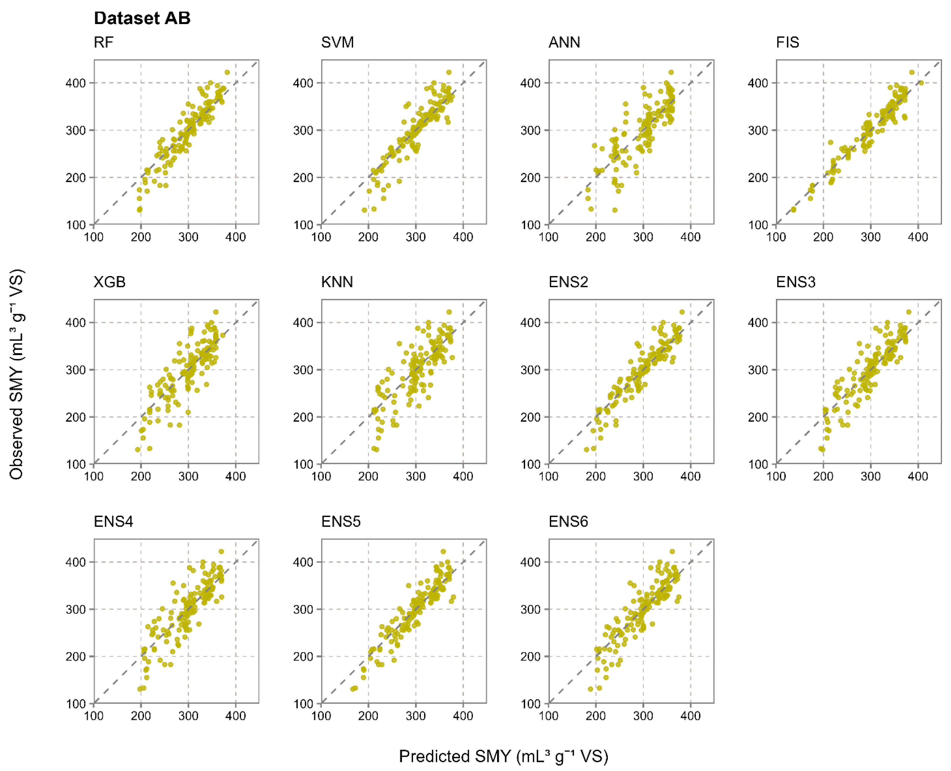
3.2. Prediction Accuracy of Evaluated Individual and Ensemble Machine Learning Models

The prediction accuracy of the evaluated individual and ensemble machine learning methods varied notably across the three used datasets for SMY prediction (

Table 2. Accuracy assessment results of individual and ensemble machine learning methods for SMY prediction.

Dataset	Prediction Method	Cross-Validation				Final Model Fit
		R2	RMSE	NRMSE	MAE	R2	RMSE	NRMSE	MAE
Dataset A	RF	0.458	44.44	0.183	36.70	0.855	27.59	0.113	21.12
	SVM	0.405	46.32	0.190	38.50	0.567	39.34	0.162	27.89
	ANN	0.358	52.28	0.215	42.93	N/A	50.04	0.206	39.43
	FIS	0.451	48.50	0.199	39.61	0.849	19.72	0.081	15.29
	XGB	0.421	52.83	0.217	42.49	1.000	1.17	0.005	0.93
	KNN	0.379	46.41	0.191	39.74	0.311	42.57	0.175	34.36
	ENS2	0.100	47.52	0.195	36.32	0.845	29.76	0.122	22.04
	ENS3	0.117	47.06	0.194	36.48	0.628	35.24	0.145	25.83
	ENS4	0.173	45.55	0.187	33.99	0.869	26.97	0.111	20.57
	ENS5	0.143	46.37	0.191	35.47	0.838	29.33	0.121	22.89
	ENS6	0.157	45.99	0.189	35.35	0.780	29.09	0.120	23.65
Dataset B	RF	0.508	30.99	0.095	23.04	0.883	17.35	0.071	12.62
	SVM	0.549	28.71	0.088	21.89	0.903	13.46	0.055	8.63
	ANN	0.392	37.07	0.114	28.37	0.580	27.22	0.112	19.38
	FIS	0.504	31.20	0.096	24.02	0.730	21.81	0.090	16.93
	XGB	0.405	34.51	0.106	26.97	0.988	4.84	0.020	3.77
	KNN	0.476	31.60	0.097	24.41	0.659	25.04	0.103	18.88
	ENS2	0.492	29.87	0.092	21.98	0.900	13.77	0.057	9.33
	ENS3	0.519	29.05	0.089	21.24	0.885	14.47	0.060	10.29
	ENS4	0.519	29.06	0.089	21.50	0.864	15.88	0.065	11.56
	ENS5	0.527	28.80	0.088	21.12	0.855	16.26	0.067	11.86
	ENS6	0.516	29.15	0.089	21.35	0.754	21.33	0.088	15.39
Dataset AB	RF	0.585	39.29	0.131	29.34	0.870	23.69	0.097	17.45
	SVM	0.602	38.71	0.129	29.05	0.837	25.41	0.104	17.19
	ANN	0.501	43.88	0.146	34.18	0.678	33.73	0.139	25.62
	FIS	0.552	42.33	0.141	32.97	0.925	16.33	0.067	12.04
	XGB	0.524	41.92	0.140	31.74	0.708	32.49	0.134	24.03
	KNN	0.567	40.08	0.133	30.65	0.655	35.14	0.145	26.83
	ENS2	0.565	39.17	0.130	28.69	0.862	22.81	0.094	16.40
	ENS3	0.560	39.40	0.131	28.98	0.787	27.89	0.115	20.83
	ENS4	0.568	39.05	0.130	28.92	0.730	31.17	0.128	23.23
	ENS5	0.610	37.08	0.123	27.33	0.868	22.41	0.092	16.98
	ENS6	0.591	37.97	0.126	28.17	0.784	28.04	0.115	20.46

Accuracy metrics indicating the highest prediction accuracy per method are bolded.

). All tuning hyperparameters of the evaluated individual machine learning methods are presented in

Table A1. Optimal tuning hyperparameters for all combinations of evaluated machine learning methods and feature selection approaches.

Dataset	Machine Learning Method	Optimal Hyperparameters
A	RF	mtry = 2, splitrule = “extratrees”, min.node.size = 5
	SVM	sigma = 0.102, C = 0.5
	ANN	size = 1, decay = 0
	FIS	num.labels = 5, max.iter = 10
	XGB	nrounds = 50, max_depth = 3, eta = 0.3, gamma = 0, colsample_bytree = 0.6, subsample = 1
	KNN	k = 7
B	RF	mtry = 3, splitrule = “extratrees”, min.node.size = 5
	SVM	sigma = 0.395, C = 2
	ANN	size = 3, decay = 0.1
	FIS	num.labels = 5, max.iter = 10
	XGB	nrounds = 50, max_depth = 3, eta = 0.3, gamma = 0, colsample_bytree = 0.8, subsample = 1
	KNN	k = 5
AB	RF	mtry = 2, splitrule = “extratrees”, min.node.size = 5
	SVM	sigma = 0.637, C = 1
	ANN	size = 3, decay = 0.1
	FIS	num.labels = 13, max.iter = 10
	XGB	nrounds = 50, max_depth = 1, eta = 0.3, gamma = 0, colsample_bytree = 0.8, subsample = 1
	KNN	k = 7

. RF and SVM, as individual machine learning methods, outperformed ensemble methods for SMY prediction according to the cross-validation results in datasets A and B, respectively. However, the ensemble approach produced a superior prediction accuracy to individual methods in dataset AB, characterized by the highest sample count and lowest number of available covariates out of the three datasets. Ensemble models also produced the lowest MAE across all three datasets, as well as the second-ranked RMSE in datasets A and B, strongly suggesting that their prediction accuracy was stable in terms of properties of the input training and test data split during cross-validation. This observation was confirmed according to the visual representation of value ranges of statistical metrics used for the accuracy assessment across 100 repetitions of 10-fold cross-validation, resulting in a total of 1000 predictions per model (Figure 3). While RF, as the most accurate machine learning model for SMY prediction in dataset A, produced an R² in the range of 0.001–0.999 and an RMSE in the range of 8.70–89.49 mL³ g⁻¹ vs. per iteration during cross-validation, the most accurate ensemble model with the lowest RMSE and MAE, ENS4, had an RMSE in the range of 40.65–49.83 mL³ g⁻¹ VS. The difference in their coefficients of variation for RMSE (0.393 for RF and 0.031 for ENS4) strongly suggests that ensemble models are much more resistant to randomness in the training/test data split during cross-validation, as well as the single split-sample approach, which was dominantly used in previous studies [16,37,38]. The same observation was confirmed when comparing coefficients of variation for RMSE of the most accurate individual and ensemble models for both dataset B (0.272 for SVM and 0.026 for ENS5) and dataset AB (0.217 for SVM and 0.021 for ENS5).

Out of five evaluated ensemble machine learning constructions, ranging from two to six individual methods in the ensemble, ENS4 was the most accurate for SMY prediction using dataset A, while ENS5 was optimal for datasets B and AB with the criterion of the lowest RMSE. While the prediction accuracy results from ENS4 and ENS5 were very close, as represented by accuracy assessment metrics, their performance proved to be a benefit of the ensemble machine learning approach in terms of model diversity, which confirmed the theoretical assumption of the ensemble approach [18]. Within these ensembles, SVM and RF were the top-two ranked individual methods for all three datasets, while FIS and KNN were also present in all optimal ensemble constructions. Besides these methods, XGB was used in optimal ensemble models for datasets B and AB, while ANN was not used in any optimal ensembles. These results confirmed the observations of previous studies on the high prediction accuracy of SVM for anaerobic digestion modeling, particularly for smaller datasets with up to 50 samples [2,13]. Its efficiency in predicting SMY did not diminish with the increase in sample count, as represented with the highest prediction accuracy of the evaluated individual methods with datasets B and AB, which contained 102 and 142 samples, respectively. RF was not as frequently used in previous studies as ANN or SVM was [5], but it regularly achieved high prediction accuracy for biogas and methane yield prediction, outperforming similar machine learning methods in a few studies [16,37]. However, the prediction accuracy of ANN in all three datasets used in this study was the lowest for datasets B and AB or second-lowest for dataset A, which is a major discrepancy with the consensus of previous studies. Since a relatively low prediction accuracy of ANN was present in a study by Wang et al. [6], who used a similar dataset with 277 samples which overlapped with datasets in this study, the previous observation that ANNs perform optimally with datasets containing a large number of samples [2] was not supported with the results of this study. Moreover, in the case of the lowest sample count in dataset A, the ANN model output a constant value for all test samples, producing a variance of predictions of zero, making R² undefined. Two likely causes of its underperformance relative to other evaluated machine learning methods might instead be its high sensitivity to noise in training data [42], which was caused by the highly heterogeneous agricultural and forest waste used for SMY production in input datasets, or the high complexity of input datasets with many covariates relative to sample count [43].

Besides cross-validation, the accuracy assessment results for all evaluated individual and ensemble models were additionally displayed for final model fitting (Table 2), since this approach was dominantly used for reporting prediction accuracy in a wide range of studies on anaerobic digestion modeling [4,5]. Cross-validation was preferred for determining the prediction accuracy and ranking of machine learning methods in this study to the final model fitting approach since the accuracy metrics produced this way do not represent the ability of machine learning models to accurately predict SMY using new data, which is characteristic for a real-case scenario [44]. While there is no theoretical foundation to completely disregard the final model fitting accuracy assessment, these data do not support the estimation of prediction accuracy using unseen data and should be interpreted as such. The cross-validation approach overcomes this limitation and is much more resistant to overfitting to the final model fitting approach [45], but the accuracy assessment from both approaches is presented in this study to clearly show the difference in statistical metrics for future studies. Presenting prediction accuracy using final model fitting might be more appealing since statistical metrics indicate a notably higher prediction accuracy than with cross-validation, but, especially for smaller datasets, such as dataset A, scatterplots (Figure A1, Figure A2 and Figure A3) clearly demonstrate overfitting for XGB and the inability of ANN to provide continuous SMY prediction. Therefore, accuracy assessment results based on final model fitting in this study are presented for the purpose of a potential comparison of contemporary results from other studies, but the comparative evaluation of the ensemble machine learning approach was solely based on the cross-validation results. The majority of previous studies also based their accuracy assessment approach on a single split-sample approach instead of cross-validation [16,37,38], which is subjected to extreme randomness in data splitting. The properties and value distribution of input training and test datasets are known to be a major determinant of prediction accuracy in anaerobic digestion modeling using machine learning, which is thus highly affected by inherent randomness in the split-sample approach [13]. Studies reporting prediction accuracy based on the single split-sample approach and final model fitting, thus frequently exhibiting R² values higher than 0.999, disregard this randomness effect and are sometimes prone to dubious conclusions on the single most accurate machine learning method based on superior R² values [2]. However, from a probabilistic standpoint based on the results presented in Figure 3, there was almost the same probability that SMY prediction based on the RF model for dataset A would produce an R² of 0.999 to produce 0.001. Comparable observations can be made for all evaluated individual methods quantified by R², RMSE, and MAE across all three datasets. These results strongly suggest that making such conclusions based on inherent randomness from a single split-sample approach can provide inaccurate observations and thus impair the ability of such machine learning models to be successfully translated to industrial-scale production [17]. The observations from this study strongly urge the adoption of a k-fold cross-validation approach in multiple repetitions as a standard in reporting the prediction accuracy from anaerobic digestion modeling in future studies, as the race to achieving the highest prediction accuracy quantified by R² on the fourth of fifth digits does not necessarily indicate a higher scientific contribution from the machine learning perspective.

3.3. Comparison of Ensemble Prediction Approach to Individual Methods and Study Limitations

Overall, the ensemble machine learning approach produced mixed results in terms of providing a higher prediction accuracy than individual methods do, achieving superior performance according to all four statistical metrics only with database AB, which had the highest number of samples and the least covariates out of the three databases. There was also no consensus on relative superiority in terms of prediction accuracy for individual or ensemble machine learning in previous anaerobic digestion modeling studies, with both individual [6,13] and ensemble models [14,46] being selected as optimal approaches in respective studies. While there were no clear observations in terms of prediction accuracy, the results from this study strongly suggest that ensemble models were much more resistant to the randomness in training and test data properties, achieving a much more stable prediction accuracy than individual methods do. It was known that ensemble machine learning reduces the risk of overfitting or underfitting in comparison to individual methods [6], but the thorough accuracy assessment in a total of 1000 iterations per model from this study quantified and confirmed this premise. A stable prediction accuracy regardless of the input data properties, with a prediction accuracy which was on-par with the best performing individual machine learning methods, is thus highly viable for automated decision-making systems on an industrial scale [47]. However, the ensemble machine learning approach produced very low R² values for dataset A, indicating issues with highly complex datasets with limited sample counts. To provide a more thorough insight into this observation, future studies on the minimum adequate sample and covariate count for major machine learning approaches are required, which was a major issue for the ANN in this study, as well as for the ensemble approach to some degree. Moreover, a focus in future research should be put on determining the minimum sample count for achieving adequate prediction accuracy using machine learning to provide maximum cost efficiency during a biochemical methane potential test. It was a frequent case that anaerobic digestion modeling studies contained fewer than 50 samples [4], which can be characterized as small datasets from the standpoint of machine learning prediction and the unknown exact minimum of samples for anaerobic digestion modeling. Despite previous studies successfully implementing similar machine learning approaches for anaerobic digestion modeling with as low as 25 input data cases [4], the results from this study suggest that too low an input sample count could be the only limiting factor in the repeatability of the evaluated approach since the number of covariates did not negatively affect prediction accuracy.

The main limitation of this study was that no new anaerobic digestion samples were created, but the use of overlapping samples as in previous studies [6] could have an advantage of exhibiting high transparency in the results, which are available to all researchers who want to verify or further optimize the results from this study. Moreover, the comparative evaluation of individual and ensemble machine learning methods was based on very heterogenous substrates from agriculture and forestry waste and simple physical pretreatment, which does not guarantee the same optimal construction of ensemble models and their prediction accuracy relative to individual methods as reported in this study. These observations were also based on mono-digestion, which is much less susceptible to fluctuations in SMY due to the use of inadequate substrates and their ratio within optimal operating conditions than anaerobic co-digestion, thus exhibiting less complexity in machine learning prediction. There is also a discrepancy in ANN prediction accuracy with the majority of previous studies, as it had the lowest prediction accuracy in this study overall but was the most frequently used machine learning method in previous anaerobic digestion modeling studies, often producing high prediction accuracy [2,4,5]. While the properties of input datasets in this study were unfavorable for ANN prediction in terms of sample count, there are many variations of artificial neural networks which could be considered before making strong observations on their effectiveness in ensemble models. As the interpretability of machine learning models for anaerobic digestion is one of key challenges in present research, previous studies explored interpretable machine learning using methods such as Shapley additive explanations (SHAPs) and local interpretable model-agnostic explanations (LIMEs) [5]. However, future studies should evaluate the interpretability of ensemble models relative to individual machine learning methods, which is currently unknown in the literature. Moreover, since there is often a discrepancy between anaerobic digestion modeling from laboratory- and industrial-scale studies [17], future studies should attempt to validate similar machine learning models using diverse real-case data.

4. Conclusions

The comparative evaluation of ensemble machine learning models according to individual machine learning methods for SMY prediction, performed using three datasets and 10-fold cross-validation in 100 repetitions, produced several notable observations which intend to narrow the research gap of optimizing ensemble model construction in anaerobic digestion modeling:

• The ensemble machine learning approach could not consistently outperform the most accurate individual machine learning method in all datasets. The ensemble approach was optimal according to all four statistical metrics, R², RMSE, NRMSE, and MAE, only for dataset AB, which consisted of the most samples and the least covariates out of the three used datasets.
• The results from a total of 1000 iterations in 10-fold cross-validation in 100 repetitions strongly suggest that ensemble models were much more resistant to the randomness in the training and test data properties during the data split, achieving a much more stable prediction accuracy than the individual methods. The coefficients of variation for RMSE from the most accurate ensemble and individual models were notably lower for the ensemble approach, with 0.393 for RF and 0.031 for ENS4 in dataset A, 0.272 for SVM and 0.026 for ENS5 in dataset B, and 0.217 for SVM and 0.021 for ENS5 in dataset AB. In dataset A, which had 40 samples, RF was the most accurate individual prediction method and achieved R² values in the range of 0.001–0.999 across 1000 iterations due to the randomness in the data split, for which the ensemble approach was much more resistant.
• Out of the five evaluated ensemble model constructions per dataset, which ranged from two to six used individual machine learning methods, ENS4 was optimal for SMY prediction from dataset A, while ENS5 was optimal for datasets B and AB. The optimal ensemble constructions generally benefited from a higher number of individual methods included, as well as from their diversity in terms of prediction principles, including decision trees, support vector machines, fuzzy inference systems, and instance-based learning. ANN was the only model which was not applied in any optimal ensemble model, struggling with input data complexity and a restricted number of input samples likely due to computational complexity and overfitting.
• A large discrepancy between accuracy assessment metrics from cross-validation and final model fitting was observed for the same models, with the final model fitting results generally indicating higher prediction accuracy and being prone to overfitting. Cross-validation was preferred for determining prediction accuracy and the ranking of machine learning methods in this study since these accuracy metrics represent the ability of machine learning models to accurately predict SMY using new, unseen data. Since the reporting of prediction accuracy based on final model fitting and the single split-sample approach is highly prone to randomness, the adoption of a cross-validation in multiple repetitions is proposed as a standard in future studies.

Due to this study’s limitations in terms of using heterogenous substrates from agriculture and forestry waste and the restriction to simple physical pretreatment and mono-digestion, future studies should be focused on widening the scope of applying ensemble machine learning to anaerobic digestion modeling. They should also focus on evaluating the interpretability of ensemble models relative to individual machine learning methods, which is currently unknown in the literature.

References

1. Andrade Cruz, I.; Chuenchart, W.; Long, F.; Surendra, K.C.; Renata Santos Andrade, L.; Bilal, M.; Liu, H.; Tavares Figueiredo, R.; Khanal, S.K.; Fernando Romanholo Ferreira, L. Application of Machine Learning in Anaerobic Digestion: Perspectives and Challenges. Bioresour. Technol. 2022, 345, 126433. [Google Scholar] [CrossRef]
2. Ling, J.Y.X.; Chan, Y.J.; Chen, J.W.; Chong, D.J.S.; Tan, A.L.L.; Arumugasamy, S.K.; Lau, P.L. Machine Learning Methods for the Modelling and Optimisation of Biogas Production from Anaerobic Digestion: A Review. Environ. Sci. Pollut. Res. 2024, 31, 19085–19104. [Google Scholar] [CrossRef]
3. Enitan, A.M.; Adeyemo, J.; Swalaha, F.M.; Kumari, S.; Bux, F. Optimization of Biogas Generation Using Anaerobic Digestion Models and Computational Intelligence Approaches. Rev. Chem. Eng. 2017, 33, 309–335. [Google Scholar] [CrossRef]
4. Khan, M.; Chuenchart, W.; Surendra, K.C.; Kumar Khanal, S. Applications of Artificial Intelligence in Anaerobic Co-Digestion: Recent Advances and Prospects. Bioresour. Technol. 2023, 370, 128501. [Google Scholar] [CrossRef] [PubMed]
5. Gupta, R.; Zhang, L.; Hou, J.; Zhang, Z.; Liu, H.; You, S.; Sik Ok, Y.; Li, W. Review of Explainable Machine Learning for Anaerobic Digestion. Bioresour. Technol. 2023, 369, 128468. [Google Scholar] [CrossRef] [PubMed]
6. Wang, Z.; Peng, X.; Xia, A.; Shah, A.A.; Yan, H.; Huang, Y.; Zhu, X.; Zhu, X.; Liao, Q. Comparison of Machine Learning Methods for Predicting the Methane Production from Anaerobic Digestion of Lignocellulosic Biomass. Energy 2023, 263, 125883. [Google Scholar] [CrossRef]
7. Song, C.; Zhang, Z.; Wang, X.; Hu, X.; Chen, C.; Liu, G. Machine Learning-Aided Unveiling the Relationship between Chemical Pretreatment and Methane Production of Lignocellulosic Waste. Waste Manag. 2024, 187, 235–243. [Google Scholar] [CrossRef]
8. Cavaiola, M.; Tuju, P.E.; Ferrari, F.; Casciaro, G.; Mazzino, A. Ensemble Machine Learning Greatly Improves ERA5 Skills for Wind Energy Applications. Energy AI 2023, 13, 100269. [Google Scholar] [CrossRef]
9. Kesriklioğlu, E.; Oktay, E.; Karaaslan, A. Predicting Total Household Energy Expenditures Using Ensemble Learning Methods. Energy 2023, 276, 127581. [Google Scholar] [CrossRef]
10. Khan, P.W.; Byun, Y.C.; Jeong, O.-R. A Stacking Ensemble Classifier-Based Machine Learning Model for Classifying Pollution Sources on Photovoltaic Panels. Sci. Rep. 2023, 13, 10256. [Google Scholar] [CrossRef]
11. Brandt, P.; Beyer, F.; Borrmann, P.; Möller, M.; Gerighausen, H. Ensemble Learning-Based Crop Yield Estimation: A Scalable Approach for Supporting Agricultural Statistics. GIScience Remote Sens. 2024, 61, 2367808. [Google Scholar] [CrossRef]
12. Mahdizadeh Gharakhanlou, N.; Perez, L. From Data to Harvest: Leveraging Ensemble Machine Learning for Enhanced Crop Yield Predictions across Canada amidst Climate Change. Sci. Total Environ. 2024, 951, 175764. [Google Scholar] [CrossRef]
13. Kovačić, Đ.; Radočaj, D.; Jurišić, M. Ensemble Machine Learning Prediction of Anaerobic Co-Digestion of Manure and Thermally Pretreated Harvest Residues. Bioresour. Technol. 2024, 402, 130793. [Google Scholar] [CrossRef]
14. Sun, J.; Xu, Y.; Nairat, S.; Zhou, J.; He, Z. Prediction of Biogas Production in Anaerobic Digestion of a Full-Scale Wastewater Treatment Plant Using Ensembled Machine Learning Models. Water Environ. Res. 2023, 95, e10893. [Google Scholar] [CrossRef] [PubMed]
15. Mohammed, A.; Kora, R. A Comprehensive Review on Ensemble Deep Learning: Opportunities and Challenges. J. King Saud Univ.-Comput. Inf. Sci. 2023, 35, 757–774. [Google Scholar] [CrossRef]
16. Wang, Z.; Wu, F.; Hao, N.; Wang, T.; Cao, N.; Wang, X. The Combined Machine Learning Model SMOTER-GA-RF for Methane Yield Prediction during Anaerobic Digestion of Straw Lignocellulose Based on Random Forest Regression. J. Clean. Prod. 2024, 466, 142909. [Google Scholar] [CrossRef]
17. Yildirim, O.; Ozkaya, B. Prediction of Biogas Production of Industrial Scale Anaerobic Digestion Plant by Machine Learning Algorithms. Chemosphere 2023, 335, 138976. [Google Scholar] [CrossRef] [PubMed]
18. Ganaie, M.A.; Hu, M.; Malik, A.K.; Tanveer, M.; Suganthan, P.N. Ensemble Deep Learning: A Review. Eng. Appl. Artif. Intell. 2022, 115, 105151. [Google Scholar] [CrossRef]
19. R Foundation for Statistical Computing. R Core Team R: A Language and Environment for Statistical Computing. Vienna, Austria. Available online: https://www.R-project.org/ (accessed on 14 October 2024).
20. Kuhn, M.; Wing, J.; Weston, S.; Williams, A.; Keefer, C.; Engelhardt, A.; Cooper, T.; Mayer, Z.; Kenkel, B.; Benesty, M.; et al. Caret: Classification and Regression Training. Available online: https://CRAN.R-project.org/package=caret (accessed on 30 November 2024).
21. Deane-Mayer, Z.A.; Knowles, J.E. Caretensemble: Ensembles of Caret Models. Available online: https://cran.r-project.org/web/packages/caretEnsemble/index.html (accessed on 30 November 2024).
22. Wright, M.N.; Wager, S.; Probst, P. Ranger: A Fast Implementation of Random Forests. Available online: https://cran.r-project.org/web/packages/ranger/index.html (accessed on 14 October 2024).
23. Karatzoglou, A.; Smola, A.; Hornik, K.; Maniscalco, M.A.; Teo, C.H. Kernlab: Kernel-Based Machine Learning Lab. Available online: https://cran.r-project.org/web/packages/kernlab/index.html (accessed on 14 October 2024).
24. Ripley, B.; Venables, W. Nnet: Feed-Forward Neural Networks and Multinomial Log-Linear Models. Available online: https://cran.r-project.org/web/packages/nnet/index.html (accessed on 14 October 2024).
25. Riza, L.S.; Bergmeir, C.; Herrera, F.; Benitez, J.M. Frbs: Fuzzy Rule-Based Systems for Classification and Regression Tasks. Available online: https://cran.r-project.org/web/packages/frbs/index.html (accessed on 14 October 2024).
26. Chen, T.; He, T.; Benesty, M.; Khotilovich, V.; Tang, Y.; Cho, H.; Chen, K.; Mitchell, R.; Cano, I.; Zhou, T.; et al. Xgboost: Extreme Gradient Boosting. Available online: https://cran.r-project.org/web/packages/xgboost/index.html (accessed on 14 October 2024).
27. Genuer, R.; Poggi, J.-M. Random Forests. In Random Forests with R; Genuer, R., Poggi, J.-M., Eds.; Springer International Publishing: Cham, Switzerland, 2020; pp. 33–55. ISBN 978-3-030-56485-8. [Google Scholar]
28. Sagi, O.; Rokach, L. Approximating XGBoost with an Interpretable Decision Tree. Inf. Sci. 2021, 572, 522–542. [Google Scholar] [CrossRef]
29. Chen, T.; Guestrin, C. XGBoost: A Scalable Tree Boosting System. In Proceedings of the 22nd ACM SIGKDD International Conference on Knowledge Discovery and Data Mining; Association for Computing Machinery: San Francisco, CA, USA, 13 August, 2016; pp. 785–794. [Google Scholar]
30. Pisner, D.A.; Schnyer, D.M. Chapter 6—Support Vector Machine. In Machine Learning; Mechelli, A., Vieira, S., Eds.; Academic Press: Cambridge, MA, USA, 2020; pp. 101–121. ISBN 978-0-12-815739-8. [Google Scholar]
31. Ding, X.; Liu, J.; Yang, F.; Cao, J. Random Radial Basis Function Kernel-Based Support Vector Machine. J. Frankl. Inst. 2021, 358, 10121–10140. [Google Scholar] [CrossRef]
32. Katal, A.; Singh, N. Artificial Neural Network: Models, Applications, and Challenges. In Innovative Trends in Computational Intelligence; Tomar, R., Hina, M.D., Zitouni, R., Ramdane-Cherif, A., Eds.; EAI/Springer Innovations in Communication and Computing; Springer International Publishing: Cham, Switzerland, 2022; pp. 235–257. ISBN 978-3-030-78284-9. [Google Scholar]
33. Jallal, M.A.; González-Vidal, A.; Skarmeta, A.F.; Chabaa, S.; Zeroual, A. A Hybrid Neuro-Fuzzy Inference System-Based Algorithm for Time Series Forecasting Applied to Energy Consumption Prediction. Appl. Energy 2020, 268, 114977. [Google Scholar] [CrossRef]
34. Zhang, Z. Introduction to Machine Learning: K-Nearest Neighbors. Ann. Transl. Med. 2016, 4, 218. [Google Scholar] [CrossRef] [PubMed]
35. Halder, R.K.; Uddin, M.N.; Uddin, M.A.; Aryal, S.; Khraisat, A. Enhancing K-Nearest Neighbor Algorithm: A Comprehensive Review and Performance Analysis of Modifications. J. Big Data 2024, 11, 113. [Google Scholar] [CrossRef]
36. Hodson, T.O. Root-Mean-Square Error (RMSE) or Mean Absolute Error (MAE): When to Use Them or Not. Geosci. Model Dev. 2022, 15, 5481–5487. [Google Scholar] [CrossRef]
37. Sonwai, A.; Pholchan, P.; Tippayawong, N. Machine Learning Approach for Determining and Optimizing Influential Factors of Biogas Production from Lignocellulosic Biomass. Bioresour. Technol. 2023, 383, 129235. [Google Scholar] [CrossRef] [PubMed]
38. Song, C.; Cai, F.; Yang, S.; Wang, L.; Liu, G.; Chen, C. Machine Learning-Based Prediction of Methane Production from Lignocellulosic Wastes. Bioresour. Technol. 2024, 393, 129953. [Google Scholar] [CrossRef]
39. Wang, Y.; Huntington, T.; Scown, C.D. Tree-Based Automated Machine Learning to Predict Biogas Production for Anaerobic Co-Digestion of Organic Waste. ACS Sustain. Chem. Eng. 2021, 9, 12990–13000. [Google Scholar] [CrossRef]
40. Jeong, K.; Abbas, A.; Shin, J.; Son, M.; Kim, Y.M.; Cho, K.H. Prediction of Biogas Production in Anaerobic Co-Digestion of Organic Wastes Using Deep Learning Models. Water Res. 2021, 205, 117697. [Google Scholar] [CrossRef]
41. Tryhuba, I.; Tryhuba, A.; Hutsol, T.; Cieszewska, A.; Andrushkiv, O.; Glowacki, S.; Bryś, A.; Slobodian, S.; Tulej, W.; Sojak, M. Prediction of Biogas Production Volumes from Household Organic Waste Based on Machine Learning. Energies 2024, 17, 1786. [Google Scholar] [CrossRef]
42. Chowdhury, M.S. Comparison of Accuracy and Reliability of Random Forest, Support Vector Machine, Artificial Neural Network and Maximum Likelihood Method in Land Use/Cover Classification of Urban Setting. Environ. Chall. 2024, 14, 100800. [Google Scholar] [CrossRef]
43. You, H.; Ma, Z.; Tang, Y.; Wang, Y.; Yan, J.; Ni, M.; Cen, K.; Huang, Q. Comparison of ANN (MLP), ANFIS, SVM, and RF Models for the Online Classification of Heating Value of Burning Municipal Solid Waste in Circulating Fluidized Bed Incinerators. Waste Manag. 2017, 68, 186–197. [Google Scholar] [CrossRef] [PubMed]
44. Bates, S.; Hastie, T.; Tibshirani, R. Cross-Validation: What Does It Estimate and How Well Does It Do It? J. Am. Stat. Assoc. 2024, 119, 1434–1445. [Google Scholar] [CrossRef]
45. Montesinos López, O.A.; Montesinos López, A.; Crossa, J. Overfitting, Model Tuning, and Evaluation of Prediction Performance. In Multivariate Statistical Machine Learning Methods for Genomic Prediction; Montesinos López, O.A., Montesinos López, A., Crossa, J., Eds.; Springer International Publishing: Cham, Switzerland, 2022; pp. 109–139. ISBN 978-3-030-89010-0. [Google Scholar]
46. Ma, Z.; Wang, R.; Song, G.; Zhang, K.; Zhao, Z.; Wang, J. Interpretable Ensemble Prediction for Anaerobic Digestion Performance of Hydrothermal Carbonization Wastewater. Sci. Total Environ. 2024, 908, 168279. [Google Scholar] [CrossRef] [PubMed]
47. Zhang, Y.; Zhao, Y.; Feng, Y.; Yu, Y.; Li, Y.; Li, J.; Ren, Z.; Chen, S.; Feng, L.; Pan, J.; et al. Novel Intelligent System Based on Automated Machine Learning for Multiobjective Prediction and Early Warning Guidance of Biogas Performance in Industrial-Scale Garage Dry Fermentation. ACS EST Eng. 2024, 4, 139–152. [Google Scholar] [CrossRef]
Figure 1. Study workflow, including six individual machine learning methods and five ensemble machine learning configurations across three datasets.
Fermentation 11 00130 g001
Figure 2. Mixed correlation plots of the three datasets used in this study, including Spearman correlation coefficients and scatterplots between SMY and all the used covariates.
Fermentation 11 00130 g002
Figure 3. Visual representation of value ranges of statistical metrics used for the accuracy assessment from 10-fold cross-validation in 100 repetitions.
Fermentation 11 00130 g003