Article

A New View on the Global Redox-Cycle of Biosphere Carbon

1
All-Russian Scientific Research Geological Petroleum Institute, Department Organic Geochemistry, Shosse Entuziastov, 36, 105118 Moscow, Russia
2
Soil, Agrochemistry & Ecology Faculty, Russian State Agrarian University—MSKhA of K.A.Timiryazev, Timiryazevskaya Str., 48, 127750 Moscow, Russia
Submission received: 17 February 2023 / Revised: 8 May 2023 / Accepted: 12 May 2023 / Published: 23 May 2023
(This article belongs to the Special Issue Permafrost and Carbon Dioxide Emission)

Abstract

:
The global carbon cycle model is presented as a natural self-regulating machine that provides renewable biomass synthesis during evolution. The machine consists of two parts, geological and biosphere. Between the parts, there is an interaction. The geological part is controlled by the movement of lithosphere plates, which is under the guidance of gravitational forces from celestial bodies acting on the Earth. The movement of the lithosphere plates is divided into a phase of a relatively quick movement, occurring in the tectonically active state of the Earth’s crust, named the orogenic period, and a phase of a relatively slow movement, occurring in the phase of the tectonically quiet state of the crust, named geosynclinal period. In the orogenic period, the energy of moving plates’ collisions is sufficient to initiate sulfate reduction, proceeding in the subduction zone. This is the reaction where sedimentary organic matter is oxidized. Resultant CO2 is injected into “atmosphere—hydrosphere” system of the Earth. Its concentration achieves maximal values, whereas oxygen concentration drops to a minimum since it reacts with the reduced sulfur forms that evolve in the thermochemical sulfate reduction and due to binding with reduced forms of metals, coming to the Earth’s surface with volcanic exhalations. Carbon dioxide initiates photosynthesis and the associated biosphere events. In the geosynclinal period, the sulfate reduction ceases, and CO2 does not enter the system anymore, though photosynthesis in the biosphere proceeds in the regime of CO2 pool depletion. Under such conditions, the surface temperature on the Earth decreases, ending with glaciations. The successive depletion of the CO2 pool results in a regular sequence of climatic changes on the Earth. The ratio of CO2/O2 is the key environmental parameter in the orogenic cycle providing climatic changes. They consistently vary from hot and anaerobic in the orogenic period to glacial and aerobic by the end of the geosynclinal period. The climatic changes provide biotic turnover. Especially abrupt changes accompany the transition to a new orogenic cycle, resulting in mass extinction of organisms and the entry of huge masses of biogenic material into the sediment. This provided the conditions for the formation of rocks rich in organic matter (“black shales”). It is shown that the suggested model is supported by numerous geological and paleontological data evidencing the orogenic cycles’ existence and their relationship with the evolution of photosynthesis.

1. Introduction

Formally, the global carbon cycle can be defined as the transformation of carbon compounds during the transition through various spheres of the Earth, including from the atmosphere to the biosphere, then to the different geospheres of the Earth’s crust and back into the atmosphere. Despite the apparent simplicity of the global carbon cycle definition, this is a complex multidimensional process involving not only the conversion of carbon compounds but also the interaction between spheres. As a result, the global carbon cycle can be indirectly influenced by the gravitational forces of the bodies of the solar system on the movement of the Earth around the Sun. The biogeochemical cycles of other elements, for example, sulfur or nitrogen, can also have an impact. Complex interactions are between geological and biosphere processes, including the process of photosynthesis, which, in addition, evolves over time. Therefore, constructing a model of the global carbon cycle is a complex and multifactorial task. We have focused our attention on two main points, the interaction of which determines the functioning of the global carbon cycle. The participation of geological processes illustrates the influence of gravity, which results in the uneven movement of lithospheric plates and the emergence of orogenic cycles. The participation of biosphere processes illustrates the role of photosynthesis and “living matter” in the global carbon cycle. At the same time, the participation of photosynthesis determines the evolution of the cycle in geological time. The link between the interaction of the geological and biosphere parts of the model is the reaction of thermochemical sulfate reduction proceeding in the subduction zone. Thanks to this reaction, the biosphere part is controlled by the geological part using carbon dioxide injections. This reaction closes the carbon cycle and ensures the emergence of a new photosynthetic cycle.
Our proposed model is fundamentally different from all the previous ones. Therefore, without going into the details that will be discussed below, we underline a few key differences. For the first time, a direct connection between geological (movement of lithosphere plates) and biosphere (photosynthesis) processes is substantiated, and a mechanism for controlling that connection through the injections of carbon dioxide into the “atmosphere-hydrosphere” system of the Earth, providing photosynthetic oscillations is described. The periodicity of changes in the ratio of the substrate (CO2) and product (O2) of photosynthesis and climatic changes during the orogenic cycle are described. An explanation is given for the biotic turnover and the periodically occurring mass extinctions of organisms related to the change of orogenic cycles. The pulsation nature of the evolution of photosynthesis and a strive of photosynthesis and the global carbon cycle, as far as oxygen accumulates in the atmosphere during the geological time to a stationary state, are shown. This state is characterized by ecological compensation point.

2. Global Carbon Cycle Model: Definition and Mechanism

2.1. The Idea of Interaction of Biosphere and Geologic Processes. The Model of the Global Cycle of Biosphere Carbon and Its Development

As early as 1926, the famous Russian naturalist Vladimir Vernadsky put forward an idea on the interaction and interconditionality of the biosphere and geological processes. Developing and concretizing his idea, we have suggested a model of the global cycle of biosphere carbon [1,
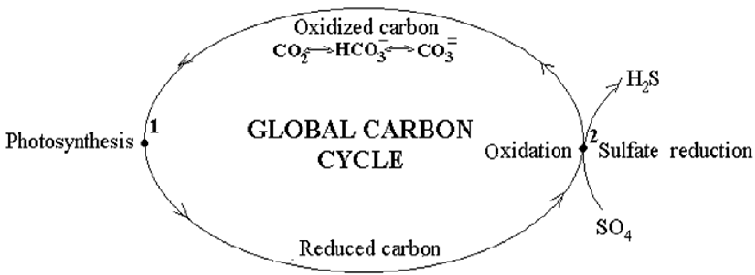
2]. According to the proposed model, carbon transformations occur along a closed loop. In the course of it, the completely oxidized state in the natural “carbon dioxide—bicarbonate—carbonate “ system transforms into a reduced state that arises during photosynthesis and the subsequent transformations, including those occurring in the earth’s crust after the burial of the “living” matter and its transition into sedimentary organic forms. The reverse transition into the initial completely oxidized state carbon makes in the subduction zone, where sedimentary organic matter is oxidized to CO2, thus ending the redox transformations in the loop (Figure 1).
The energy for the carbon transition into the reduced state in photosynthesis is provided by the sun. The energy for the carbon oxidation in reverse transition is taken from the energy evolved in collisions of the oceanic lithosphere plates with the continental plate, on which organic matter is deposited. The collisions of lithosphere plates occur in the subduction zone. It is important to stress that the cycle is called biosphere one since it is assumed that the carbon of carbonate thicknesses does not participate in the global carbon cycle because of its extraordinarily low rate in the reactions of chemical exchange as compared with the rates of other components of the natural “carbon dioxide-bicarbonate-carbonate” system [1].
The carbon cycle can be formally considered as a virtual natural self-regulated machine, which finally provides the renewable synthesis of biomass in the course of the evolution. The machine consists of geological and biosphere parts. The geological part comprises the permanently moving lithosphere plates performing irregular motion, which, according to the hypothesis, occur due to the gravitational interaction of celestial bodies with the Earth. Two phases are distinguished in motion [1,2]. The short-term phase of relatively quick motion accompanied by frequent collisions is called an orogenic period. It is characterized by intense volcanism, magmatism, and mountain building. The long-term phase of slow motion, accompanied by rare collisions, occurs in the quiet state of the Earth’s crust when flattening and weathering become dominant. This phase is called the geosynclinal period.
The interaction between celestial bodies is one of the theories, and not the only one; in fact, there is also a theory of internal terrestrial processes. However, in any case, this origin is not essential from the point of view of the discussion and conclusions set out in the text.
The geological part is a leading one since it determines the duration of both periods of the geological part. The impact of the processes in the geological part of the model on its biosphere part is transmitted via the injections of CO2, which arise during the oxidation of sedimentary organic matter in the reaction of thermochemical sulfate reduction occurring in the subduction zone. The subsequent CO2 distribution over the planet initiates photosynthesis and coupled biosphere processes. In the orogenic period, while oxidation of organic matter goes on, the CO2 concentration in “atmosphere—hydrosphere” system is maximal, providing a maximal photosynthesis rate.
In the geosynclinal period, when the number and the intensity of collisions of lithosphere plates decrease, it causes a sharp decline in the intensity of sulfate reduction and slowing of CO2 flux into the “atmosphere—hydrosphere” system. The concentration of CO2 in the system drops, causing the corresponding reduction of the photosynthesis rate. It leads to the conclusion that in the geosynclinal period, photosynthesis functions under CO2 pool depletion.
Due to repetitive orogenic cycles, the above means that evolution of photosynthesis is not continuous, but occurs in the form of pulsations, caused by the filling of the Earth’s “atmosphere-hydrosphere” system with CO2 during the orogenic period of the cycle and its depletion during the geosynclinal period.
Before considering the operation of the virtual machine under study, it is necessary to understand how global photosynthesis works in large systems and how it differs from conventional photosynthesis in an “environment—plant leaf” system.

2.2. Global Photosynthesis in Large Systems: Its Description and Properties

As follows from the above, each orogenic cycle in a geologic part of the virtual machine generates a photosynthesizing cycle in its biosphere part. Photosynthesis in large systems (global photosynthesis), unlike photosynthesis of an individual organism of C3 type (conventional photosynthesis), represents generalized characteristics of the photosynthetic activity of all organisms living at the moment and has all the properties of photosynthesis of an individual organism, excepting the ability to ontogenesis [3]. They include the presence of CO2 assimilation and photorespiration. The first process is reciprocal to the second. The CO2 assimilation is responsible for the accumulation of organic matter (biomass) in the sediment, whereas the photorespiration is responsible for its decrease.
Like conventional photosynthesis, global one has the ability to fractionate carbon isotopes. An increase in the CO2/O2 concentration ratio in the environment stimulates CO2 assimilation and, hence, the organic matter accumulation in sediment, while the reduction in the CO2/O2 concentration ratio stimulates photorespiration and leads to a decrease in the accumulation. Accordingly, the increase in CO2 concentration in the orogenic period of the cycle results in the 12C enrichment of organic matter, while the increase of oxygen concentration in the course of the geosynclynal period results in the gradual enrichment of organic matter in 13C. The organic matter most enriched in 12C is observed in the orogenic period of the cycle, whereas the maximal 13C enrichment is achieved by the end of the geosynclinal period. Formally, the photosynthesis of an individual organism is usually described by Equation (1).
CO 2 + H 2 O   h ν   ( CH 2 O ) + O 2  
Here, the left side of the equation shows the carbon dioxide and the water necessary for photosynthesis; the source of them is the environment; hv denotes the energy of the sun; (CH2O) is the product of photosynthesis, formally denoting the biomass produced during photosynthesis; O2 denotes oxygen, the second product of photosynthesis.
It is shown [3] that photosynthesis in large systems, under certain assumptions, can be described by a similar equation. Let us see first what is understood as biomass for the biosphere. To do this, we will use the concept of “living” substance, introduced by Vladimir Vernadsky [4]. It is obvious that biomass consists of autotrophic (photosynthetic) and heterotrophic parts.
“living” substance = photosynthetic biomass + heterotrophic biomass
Both parts of the “living” matter can be considered photosynthesis products if the heterotrophic part is taken as a secondary product obtained by using photosynthetic biomass in the food chain. At the same time, oxygen released during the formation of the primary product, before its part was used for the synthesis of heterotrophic biomass, accumulates in the atmosphere.
Thus, the equation of global photosynthesis for the biosphere can be rewritten [3] as follows:
CO2 + H2O = “living” matter + O2 atmosphere
Similarly, Equation (3) of global photosynthesis can be written for the system of the global cycle of biosphere carbon as Equation (4):
CO2 + H2O = “living” matter + COM sediment + O2 atmosphere
The difference between Equations (3) and (4) is in the fact that in the right part of (4), as an analog of biomass, the “living” matter appears to be the sum of “living” matter and sedimentary organic matter. Obviously, the first term is much less as compared with the second and can be neglected. Atmospheric oxygen will also include the oxygen that replenishes the atmosphere at all stages of photosynthesis of both primary and secondary (heterotrophic) products over the same period.
Given the above approximations, Equation (4) presenting photosynthesis for the global carbon cycle system can be shown as follows
CO2 + H2O = COM sediment + O2 atmosphere
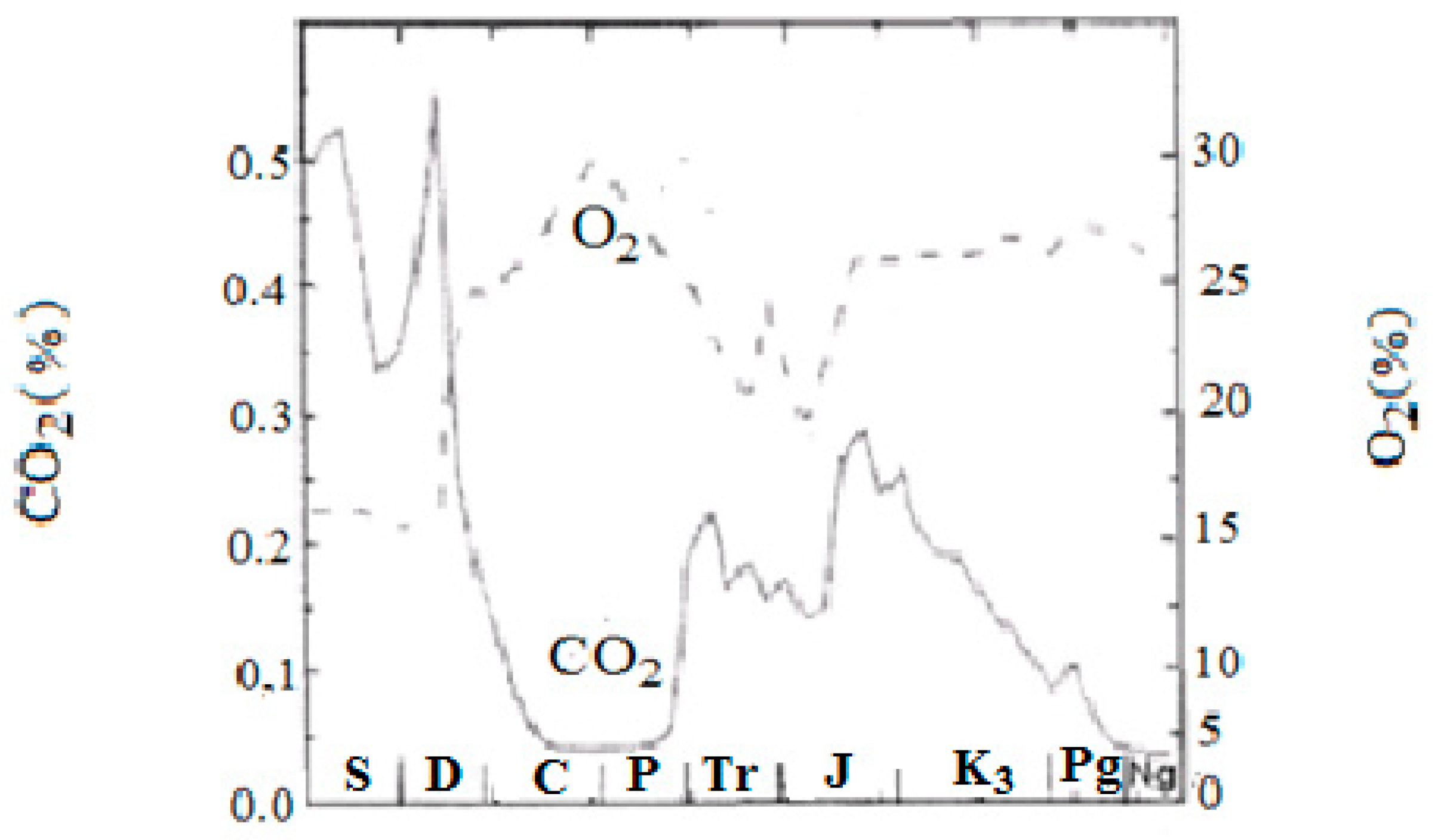
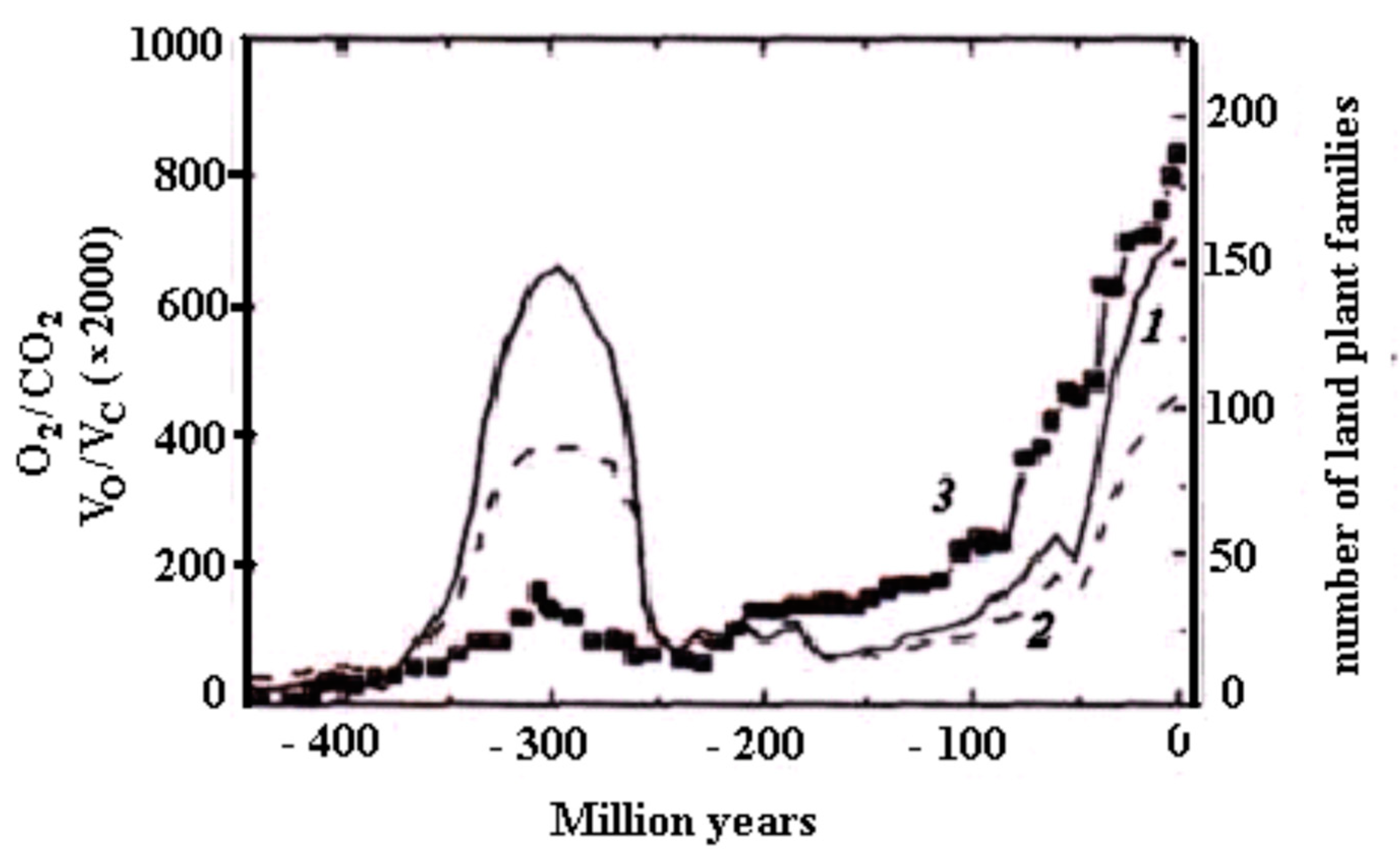
The validity of using Equation (5) for a description of photosynthesis in the global carbon cycle is proved by the fact that the parameters of global photosynthesis, operating in the global carbon cycle, analogs of the parameters of conventional photosynthesis in the Equation (1), i.e., the relationship between substrate and product (CO2 and O2) of photosynthesis is anti-phase, while the relationship between photosynthesis products (CH2O and O2) is in-phase.
Indeed, Figure 2 demonstrates the anti-phase relationship between CO2 and O2 in the Phanerozoic, calculated by means of the Geocarb III model. 
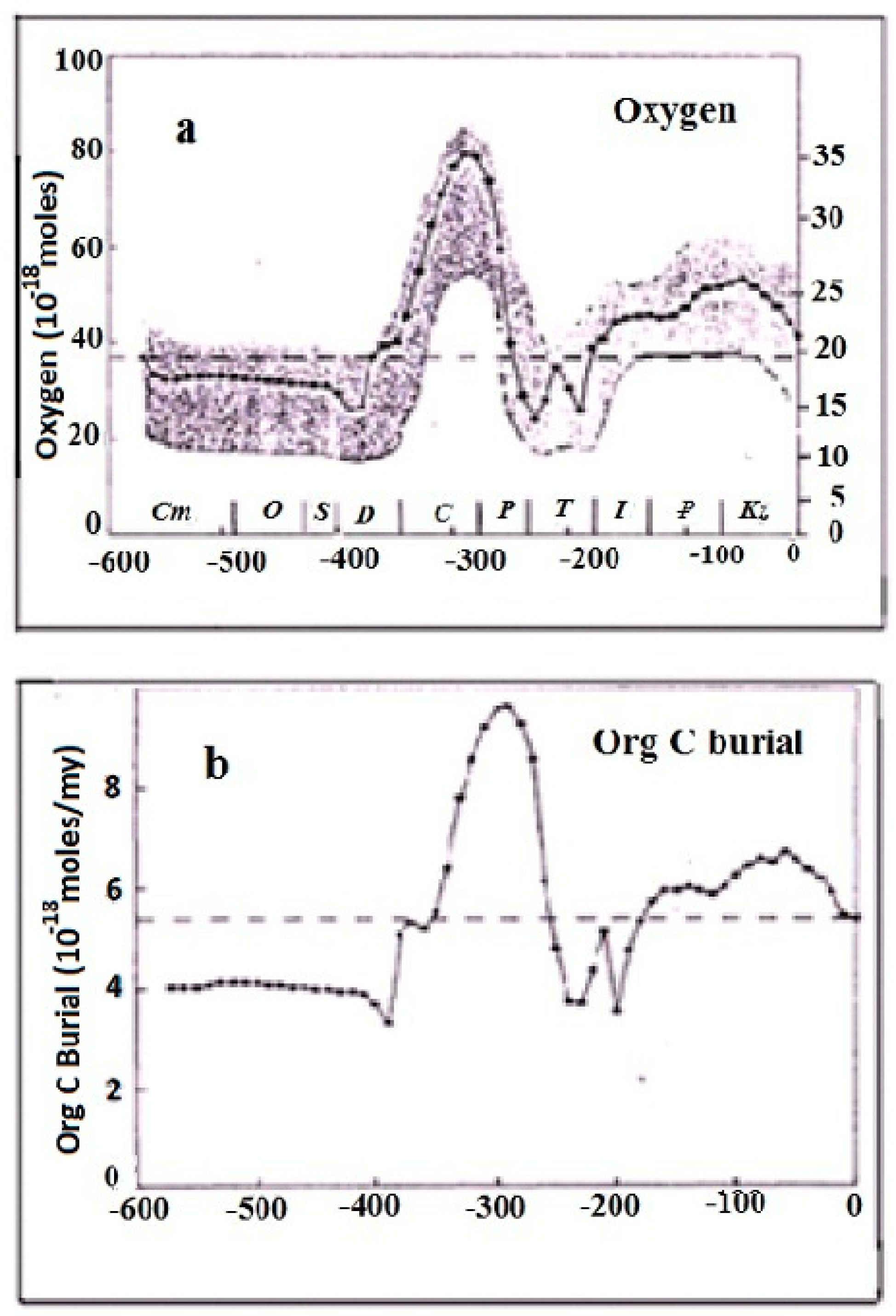
Figure 3 demonstrates the in-phase relationship between oxygen content in the atmosphere and sedimentation rate in the Phanerozoic.

2.3. The Influence of Geologic Processes on Global Photosynthesis Is Carried out via the Oxidation of Sedimentary Organic Matter in the Subduction Zone: The Ecological Compensation Point

Having found out the meaning of the term “global photosynthesis”, it is time to proceed considering the work of the biosphere part of the natural virtual machine, where global photosynthesis plays a key role. The analysis of the biosphere part functioning begins with the reaction of sedimentary organic matter oxidation in the subduction zone. It can be presented as follows:
SO4 = + 2 CH2 O => 2 CO2 + 2H2O + S = −Q
The term designated as (CH2O) means organic matter accumulated on the continental plate during all preceding orogenic cycles. Organic matter acts as a reducing agent, and the bound oxygen of gypsum (SO4 =), formed from the sulfate of marine waters, acts as an oxidizer. The carbon dioxide evolved in the reaction is injected into the atmosphere and carried over the planet, initiating photosynthesis. Another reaction product, hydrogen sulfide (S=) also rises to the surface, but being more reactive than CO2, binds with oxygen, accumulated in the preceding geosynclinal period decreasing its concentration in the atmosphere. Oxygen is also bound by the reduced forms of metals from igneous rocks that rise to the Earth’s surface with volcanic exhalations. It should be emphasized that the reaction under study is the main point of coupling geological processes with biosphere ones.
In the present work, the subduction is considered only between the oceanic and continental lithospheric plates since the sedimentary organic matter is accumulated mainly on the continental plates, which is further oxidized.
As said before, the biosphere part of the natural virtual machine is under the guidance of the geological part since the lithospheric plates’ movement determines the duration of the orogenic and geosynclynal periods of the cycle. At the same time, variations in global photosynthesis within the orogenic cycle cause climatic and associated changes in the biosphere.
As noted earlier, the properties of global photosynthesis, as well as the properties of conventional photosynthesis, depend on the CO2/O2 ratio in the environment. The ratio changes in the course of the orogenic cycle. In the orogenic period of the cycle, when the sulfate reduction proceeds, “the atmosphere—hydrosphere” system is filled with CO2. Its concentration achieves maximum. Taking into account the shortness of the orogenic period, as compared with the geosynclinal one, we have accepted that the concentration of CO2 in the orogenic period is maximal and constant.
In the geosynclinal period, the intensity of the sulfate reduction reaction slows down sharply, causing a considerable reduction of CO2 flux from the subduction zone. At the same time, thanks to photosynthesis, the CO2 consumption goes on. It allows concluding that global photosynthesis within the geosynclinal period functions under the condition of CO2 pool depletion achieving minimal CO2 concentration by the end of the period. It means that photosynthesis works in a periodic mode.
To answer the question of how the concentration of O
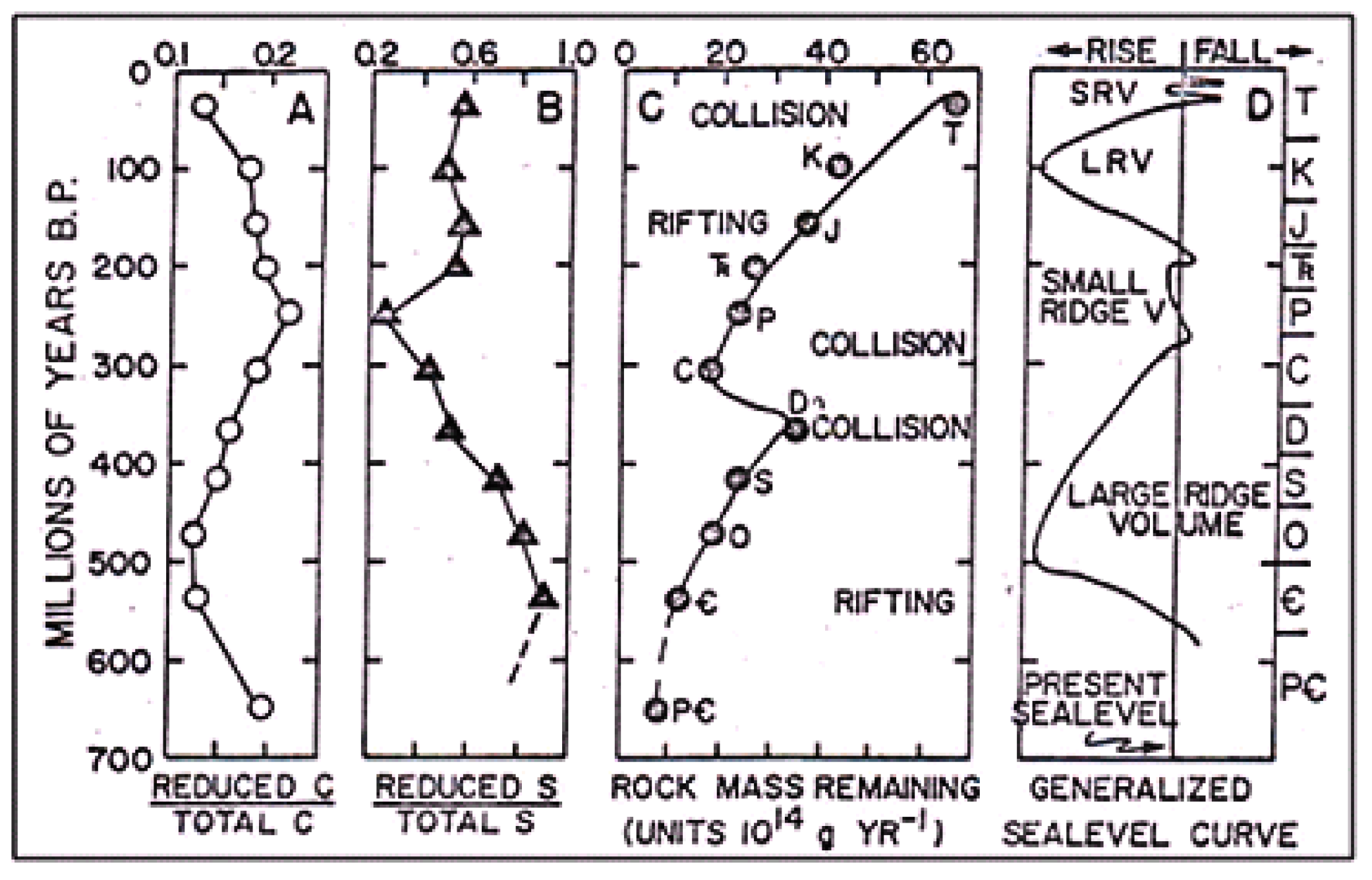
2 changes during the repetitive orogenic cycles (in the course of geological time), let us turn to Table 1. It is easy to see that with the emergence of photosynthesis, the oxygen concentration first increases rapidly, reaching the maximum values in the middle of the Phanerozoic (Carboniferous/Permian period). Then, it decreases slightly. Taking into account the present oxygen concentration in the atmosphere (~21%), it can be assumed that the oxygen concentration strives to stationary values over time.
Accordingly, the accumulation of organic matter in the Earth’s crust began to decrease, which occurred synchronously with an increase in the oxygen content in the atmosphere. As already mentioned, the predominance of the assimilation component in global photosynthesis entails the enrichment of carbon of organic matter with the isotope 12C, while the predominance of the photorespiratory component leads to the enrichment of organic matter with the isotope 13C. The described mechanism of accumulation of sedimentary organic matter in the Earth’s crust and oxygen in the atmosphere is reflected in the observed isotopic enrichment of carbon of sedimentary organic matter in isotope 13C with time [15].
In the course of repetitive orogenic cycles, with each new cycle, the photorespiration contribution has increased, while the contribution of CO2 assimilation decreased. This meant that the increment of sedimentary organic matter (the newly formed organic matter) in the Earth’s crust was decreasing, but the total amount of organic matter has increased, though at a lesser rate. In the same way, the increment of O2 has decreased, but the total content of oxygen in the atmosphere has increased at a lesser rate.
This situation continued until the contribution of CO2 assimilation became equal to the contribution of photorespiration. Simultaneously, the system of the global carbon cycle came to a stationary state. It meant the system had reached an ecological compensation point (like a state of a compensation point in conventional photosynthesis).
Resuming the obtained results of the consideration of the biosphere part of the natural virtual machine (the global cycle of biosphere carbon), it can be argued that global photosynthesis developed from cycle to cycle in the form of pulsations. More exactly, pulsations have appeared with the advent of oxygen in the atmosphere and coupled photorespiration. In other words, global photosynthesis in the long-term geosynclinal period of the cycle evolved in conditions of CO2 pool depletion. This allowed concluding on the emergence of the isotope Rayleigh effect, which conditions carbon isotope fractionation within the geosynclinal period of the cycle and determines the isotope composition of organic and carbonate carbon in the cycle. In particular, the produced sedimentary organic matter turned out to be the most enriched in 12C in the orogenic period, whereas in the geosynclinal period, it was getting enriched with 13C, achieving maximal values by the end of the period.
In the course of repetitive orogenic cycles, the described evolution of global photosynthesis eventually leads to a stationary state, when the amount of organic carbon produced during photosynthesis becomes equal to the amount of carbon returned back to the oxidized state. From this moment, the accumulation of organic matter in the Earth’s crust and oxygen in the atmosphere no longer occurs.
Thus, the evolution of global photosynthesis during repetitive cycles ensures the achievement of stationary levels of oxygen concentrations in the atmosphere close to the maximum. Sedimentary organic matter in each new cycle differs in its composition from the composition synthesized in the previous cycle. This is caused by a higher level of oxidation in the environment and a higher level of evolution. The latter means that changes in the composition of “living matter” are associated with adaptive changes in the biomass of living organisms to a higher level of oxygen concentration, increasing with time.

2.4. The Coupled Changes of Global Photosynthesis and Environmental Parameters within the Orogenic Cycle

As shown in the previous section, the evolution of global photosynthesis in the biosphere part of the virtual machine begins with the arrival of CO2 as a result of thermochemical sulfate reduction, where sedimentary organic matter is oxidized in the subduction zone. The rate of global photosynthesis depends on the concentration of the reaction substrate (CO2); the concentration of another substrate, H2O (before the appearance of terrestrial life), is considered to be excessive, i.e., not rate-limiting. Since oxygen (O2) is one of the products of global photosynthesis, it is convenient to determine the evolution of global photosynthesis in the orogenic cycle via the variations of the CO2/O2 ratio. It varies in the cycle from the maximum value at the beginning of the cycle (in the orogenic period) to the minimum value at its end (at the end of the geosynclinal period).
Let us see now the coupled variations of the global photosynthesis evolution and environmental and life parameters within the orogenic cycle.
In the orogenic period of the cycle, when the oxidation of sedimentary organic matter in the subduction zone intensively occurs, the CO2 concentration in the “atmosphere–hydrosphere” system on the Earth reaches its maximum. Taking into account the “greenhouse effect”, it is obvious that surface temperatures on the Earth in this period achieve their maximum values.
In the geosynclinal period, the sulfate reduction in the subduction zone slows down, whereas global photosynthesis goes on. Hence, the CO2 concentration begins to decrease. By the end of the geosynclinal period, the lowest temperature is reached, and glaciations occur. In parallel with the temperature decline due to photosynthesis, the oxygen concentration in the atmosphere increases. It means the CO2/O2 concentration ratio in the “atmosphere–hydrosphere” system declines in parallel with CO2 concentration. Accordingly, the CO2/O2 ratio achieves its minimum at the end of the geosynclinal period. Thus, one can see that all environmental characteristics vary within the orogenic cycle simultaneously with photosynthesis variations.
Thus, in the biosphere part of the virtual machine, the evolution of global photosynthesis within a separate orogenic cycle is accompanied by simultaneous and coupled variations of environmental parameters: temperature, oxygen and carbon dioxide content, and the CO2/O2 ratio. In addition to the aforementioned environmental parameters, so-called life parameters change, which are dependent on environmental parameters.
Gorikan and co-authors [16] have investigated radiolarians, which are single-celled organisms with a wide range of adaptive capabilities. Among them, there were species that dominated in an anaerobic environment and at elevated temperatures, i.e., under conditions typical to the orogenic period. The other species dominated in an oxygen environment and at low temperatures, i.e., dominated in conditions that corresponded to the geosynclinal period of the cycle. The studied group of radiolarians included 60 genera, including 157 species.
As a model of the orogenic cycle, the authors considered a geological time interval in the Jurassic Pliensbachian—Toarcian, in which climatic oscillations have occurred, one phase of which (Pliensbachian) was analogous to the geosynclinal period of the orogenic cycle, the other (Toarcian) was analogous to the orogenic period of the cycle.
The dominance of thermophilic anaerobes in the “orogenic” period was replaced by the dominance of cold-resistant anaerobes by the end of the “geosynclinal” period. This corresponded well to the changes in temperature and CO2 concentration expected from the model—from a maximum in the orogenic period to a minimum by the end of the geosynclinal period. Oxygen concentration changes occurred in the opposite direction from the minimum O2 concentration in the orogenic period to the maximum by the end of the geosynclinal period.
Thus, the data obtained by Gorican and co-authors (16) confirm the connection between the evolution of “living” organisms and, hence, the chemical composition of sedimentary organic matter with changes in environmental conditions.
One more life parameter bound to the changes in CO2/O2 concentration ratio within the orogenic cycle is the carbon isotope ratio of sedimentary organic matter. As said before, the carbon isotope ratio of organic matter depends on the contribution of CO2 assimilation and photorespiration to global photosynthesis.
The greater the contribution of CO2 assimilation to global photosynthesis, the more sedimentary organic matter is enriched in 12C. On the contrary, the greater the contribution of photorespiration, the more the enrichment of organic matter in 13C. An indicator of the contribution of the photosynthesis evolution is the CO2/O2 ratio, the change of which, in the cycle, was discussed above as it follows from the previous consideration, the most “light “ carbon isotope composition organic matter has in the orogenic period. In the geosynclinal period, when the CO2/O2 ratio begins to decrease because of the cessation of the influx of CO2 from the subduction zone, the organic matter is enriched in 13C.
Hayes [17] has suggested using another life parameter based on carbon isotope composition. It is an analog of modern 13C discrimination used in conventional photosynthesis. The parameter defines the difference between the carbon isotope composition of synthesized biomass and that of CO2. Based on the actualism principle, he proposed to express 13C discrimination in the past, as follows:
Δ = δ13Corg − δ 13Ccarb
where Δ 13C discrimination in the past is the difference between the carbon isotope composition of sedimentary organic matter and that of carbonates coeval to this organic matter; δ13Corg is the carbon isotope ratio of sedimentary organic matter, which is the analog of biomass; δ 13Ccarb is carbon isotope ratio of carbonates, coeval to organic matter. It is an analog of CO2.
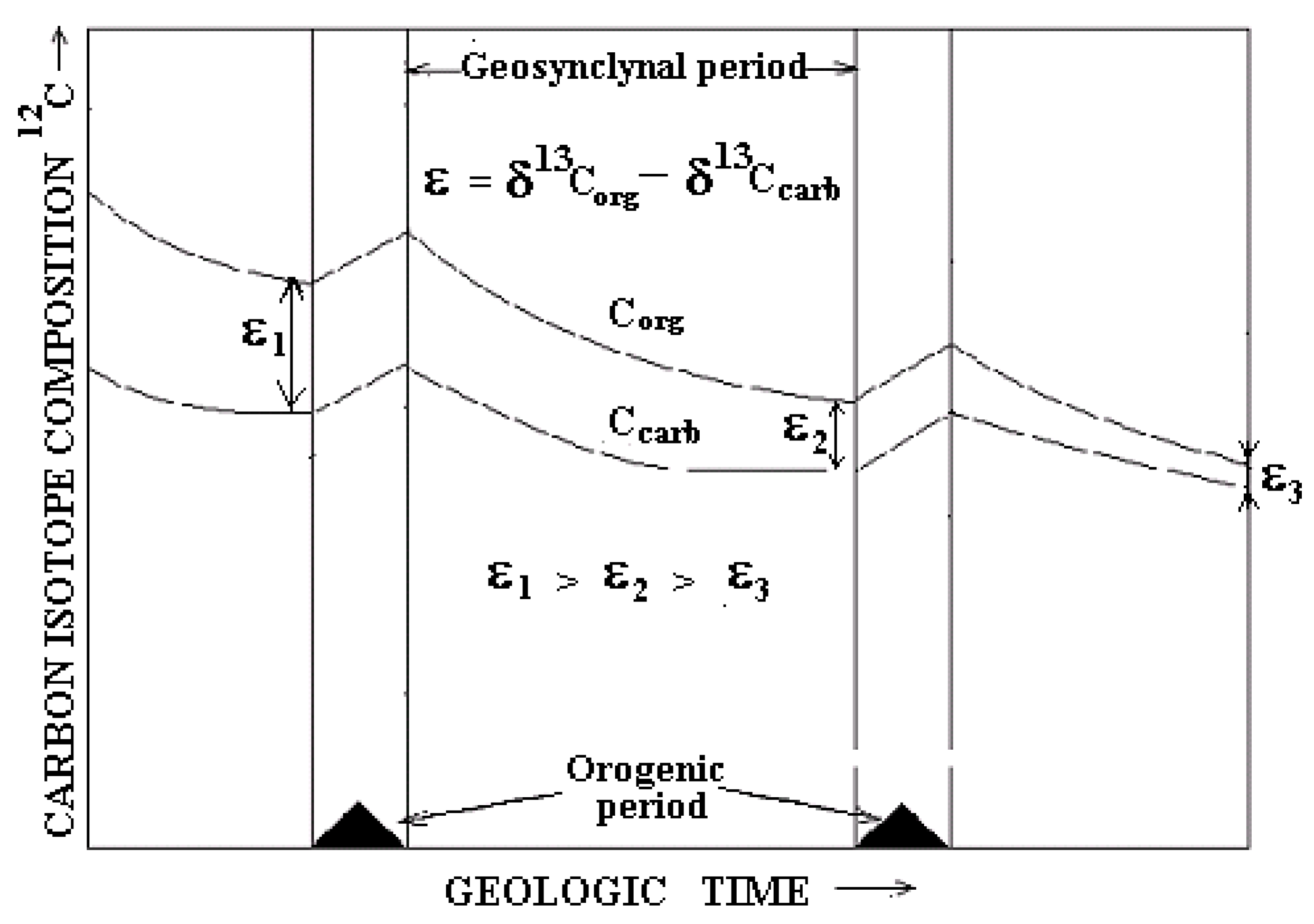
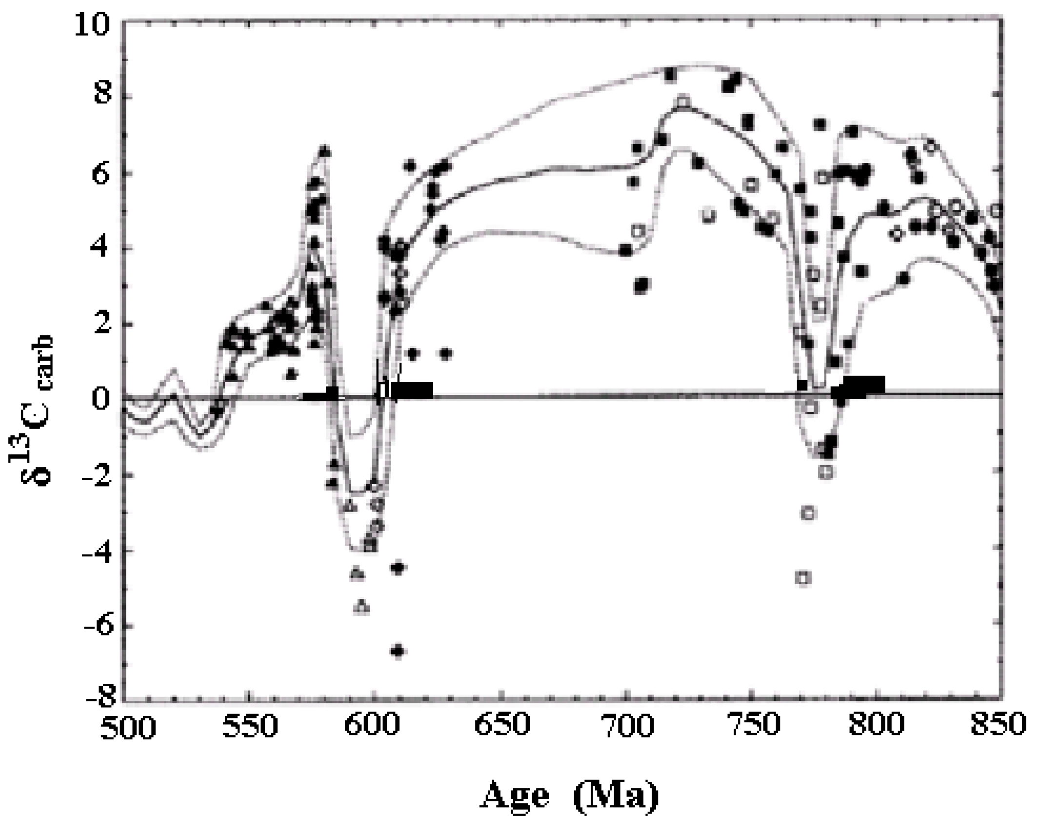
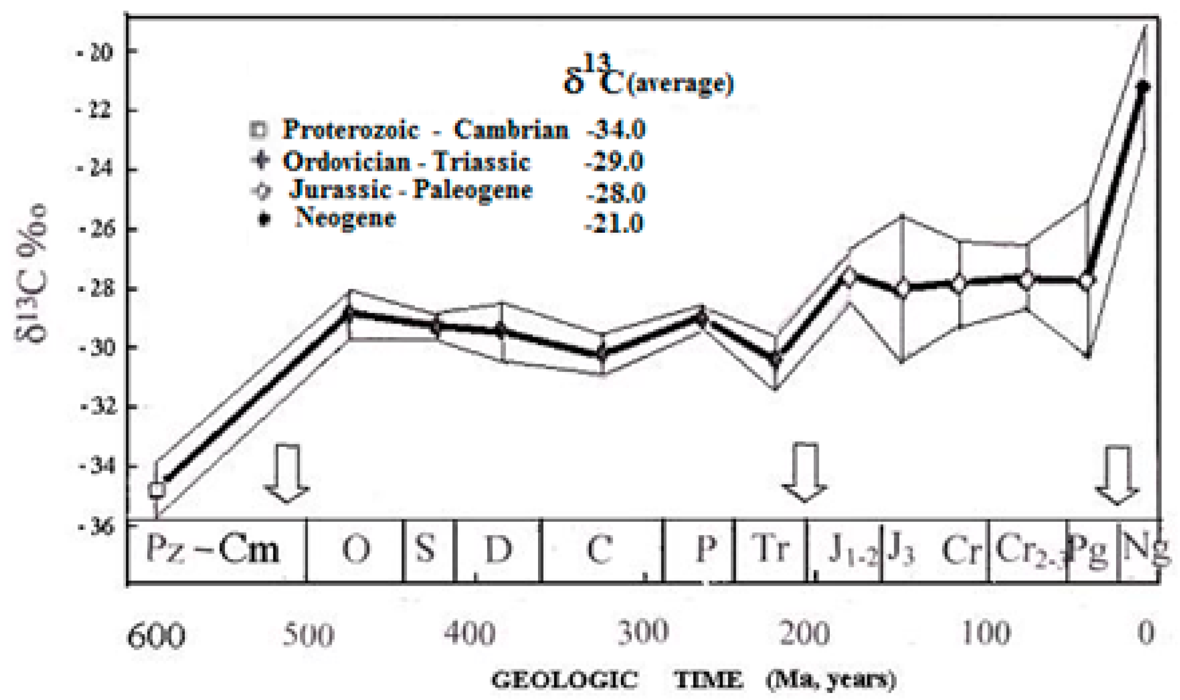
How does Δ 13C discrimination vary within the orogenic cycle? Since the CO2 concentration in the geosynclinal period of the cycle decreases, then under the action of Rayleigh isotope depletion effect, the δ13Corg and δ 13Ccarb values become more positive. The increase of O2 content within the orogenic cycle due to photosynthesis makes additional enrichment of organic matter in 13C. The value δ13Corg becomes more positive. As a result, the value Δ13C becomes lesser by the end of the cycle.
Considering the trend of Δ13C change in repetitive orogenic cycles and taking into account the progressive increase of oxygen content in the atmosphere, one can conclude that 13C isotope discrimination in the past should decrease step by step, as shown in Figure 4; this trend is supported by the observed enrichment in 13C of sedimentary organic matter with time [15].
In conclusion, I can say that the considered material allows asserting that in spite of variations of global photosynthesis within the orogenic cycle, the general trend with time shows that the evolution of global photosynthesis went on in the pulsation regime step by step.
This happened until the evolution of photosynthesis brought the global carbon cycle system to the point of ecological compensation. As shown in the work [1], this took place in the Miocene, when a new C4 type of CO2 assimilation appeared. The biological sense of it is in the fact that such evolution helped to select and to consolidate useful properties for the adaptation of organisms to varying conditions.
Of course, the proposed model is just an approximation of the description of the real situation. However, in the following part of the paper, we will show that it is a good approximation.

3. Arguments and Facts Substantiate the Model of Global Redox Cycle of Biosphere Carbon

3.1. The Proof of the Link of Sedimentary Organic Matter Oxidation with Thermochemical Sulfate Reduction in the Subduction Zone

One of the key model’s positions asserts that the interaction between the geological and biosphere parts of the machine is carried out through the oxidation of sedimentary organic matter in thermochemical sulfate reduction. Oxidation occurs when lithospheric plates collide in the subduction zone. Let us see what experimental data indicate the binding role of the above reaction between the geological and biosphere parts of a virtual machine. Mackenzie and Piggot [18], examining the variations of the isotope composition of carbon in marine carbonates and that of sulfur in marine gypsum, found that the secular curves, illustrating the variations of the above isotopic characteristics in the Proterozoic and in the Phanerozoic, have the form shown in Figure 5.
The curves in Figure 5 reflect consistent changes in time of carbon isotope composition in carbonates dissolved in seawater, and sulfur isotope composition of gypsum, the source of which is sulfate from oceanic water. The curves reveal two oppositely directed humps. Next to each of them, the authors indicated the most commonly spread minerals at that moment. The lower hump corresponds to carbonates and pyrite, formed from CO2 and H2S. It allows concluding that the minerals of the lower hump are formed from the sulfate reduction products in the orogenic period, whereas the minerals corresponding to the upper hump are associated with the substrates of the reaction in the geosynclinal period.
Compare now how the conclusions based on the chemical data are consistent with those stemming from isotopic data. First, let us see data on sulfur isotope fractionation in sulfate reduction reactions. To understand what causes isotopic variations of sulfur, some comments are needed. The fact is that thermochemical sulfate reduction is accompanied by the fractionation of sulfur isotopes [19,20]. Since the process is periodic, it proceeds with the depletion of sulfate (substrate) and is followed by the enrichment of sulfate in 34S due to the Raleigh isotope effect. This means when 34S enrichment is observed, sulfate reduction occurs. This, in turn, allows concluding it is the time of the orogenic period of the cycle.
During the period corresponding to the upper hump, the isotope composition of sulfate sulfur is shifted towards enrichment in 32S. This means at the moment under study, the geosynclinal period takes place. Thus, the consideration of sulfur isotope fractionation during the thermochemical sulfate reduction leads to the same conclusions, which stem from the analysis of the prevalence of the corresponding minerals.
It also follows from Figure 5 that when sulfate sulfur is enriched in 34S, the carbon of marine carbonates is enriched in isotope 12C. This synchronicity in the isotopic changes of sulfur and carbon is also explained within the adopted approach. However, one more remark is needed.
Accounting for the completeness of the sedimentary organic matter oxidation in the subduction zone, the carbon isotope composition of the resultant CO2 completely inherits that of organic carbon. With respect to the time of origin of the lower hump (orogenic period, as shown above), it can be argued that the enrichment of sulfates in 34S means that a large amount of CO2, enriched in 12C, enters the marine “carbon dioxide—bicarbonate—carbonate” system making its total carbon enriched in 12C. Obviously, an opposite picture of isotopic changes of sulfur and carbon should be observed in this period as well.
On the contrary, with respect to the upper hump, the reasoning on the isotopic variations of sulfur and carbon based on the same logic leads to conclusions that fully coincide with those made on the chemical data. It is the time of the geosynclinal period.
According to another argument [21], it was suggested that at low oxygen concentrations in the Precambrian atmosphere, some amount of H2S achieved the Earth’s surface. It was the reason for the widespread sulfide-oxidizing bacteria. The prevalence of sulfide-oxidizing bacteria was so great that the authors of the mentioned work came to the conclusion that bacterial biomass was the main supplier of sedimentary organic matter at that time. This, in turn, is indirect evidence for thermochemical sulfate reduction occurring in the subduction zone.

3.2. The Changes of Geological Characteristics Reflect the Regular Changes in Photosynthesis Conditions within the Orogenic Cycle

One of the statements of the model is the change in photosynthesis evolution during the orogenic cycle is expressed as the variations in the concentration ratio of CO2/O2. It is accepted that during the short-term orogenic period, the above ratio quickly achieves constant and maximal value. It remains such throughout the entire period. With the beginning of the long-term geosynclinal period, the CO2 concentration decreases from the maximal value at the onset of the period up to the minimal value at its end. This means that over the time of the geosynclinal period, photosynthesis works under CO2 pool depletion.
Changes in photosynthesis conditions within the orogenic cycle were accompanied by significant climatic changes and related biosphere events. High temperatures of the orogenic period were replaced by low temperatures of the geosynclinal period up to glaciations at its end. There was a transition from the ipoxic (or low-oxygen) conditions of the orogenic period to the aerobic conditions of the geosynclinal period. The described changes in the habitat led to a corresponding biotic turnover within the geosynclinal period [16].
The periodic variations of photosynthesis conditions in the repetitive orogenic cycles are imprinted in the geological and paleontological chronicle in the form of periodic sea-level fall and rise in the form of fluctuations of various geological parameters [18]. Some of them are demonstrated in Figure 6.
Changes in photosynthesis conditions during repeated orogenic cycles are reflected in changes in a number of geological parameters, shown in Figure 6.
The first two curves demonstrate the relationship between carbon and sulfur global cycles considered before. Curve A presents the changes in the concentration ratio of the reduced forms of carbon (organic carbon) to the total carbon (organic + carbonate carbon) in sedimentary rocks. The second curve (B) describes the changes to the ratio of the concentration of the reduced sulfur (sulfides) to the total sulfur (pyrite and gypsum sulfur). From the comparison of both curves, it follows that they display counter-phase variations. The first variable may be regarded as an analog of organic matter content in the sedimentary rocks, while the second is an analog of the reduced sulfur content in the rock. The first variable may be considered as a substrate of sulfate reduction, and the second as its product. This explains the counter-phase character of their variations.
Curve C describes the geological variable presented by the relative change in the mass of sedimentary rocks for some conventional unit of geological time. The curve discloses the link between the sedimentary rock mass, preserved with tectonic plate movements and major continental plate collisions, and active rifting [18].
Curve D presents the sea level variations as a function of geological time. As we can see from Figure 6, the sea level goes up with the growth of the mid-oceanic ridge volume and vice versa [18]. The authors bound them to plate movement and intense magma entry to the Earth’s surface, accompanied by the new plate formation.

3.3. The Carbon Isotope Composition of Marine Carbonates Reflects the Regular Sequence of Changing Conditions of Photosynthesis within the Orogenic Cycles

Some researchers who studied the Proterozoic have pointed out the relationship between the amount of sedimentary organic matter and O2 content in the atmosphere [22], the relationship between carbon isotope composition of organic matter and glaciations [21]. The others have revealed the relationship between the oxygenation of the”ocean—atmosphere “ system and glaciations [22,23,24]. As one can see from the model described before, all the above parameters are connected together.
The carbon isotope composition of marine carbonates refers to those environmental parameters that, changing in parallel with the conditions of photosynthesis, make it possible to control them throughout the entire orogenic cycle. Given that during the orogenic period, sedimentary organic matter is fully oxidized in the subduction zone, its carbon isotope composition is inherited by CO2 completely without changes. This is the reason for the “light” isotope composition of all carbon components of the natural “carbon dioxide—bicarbonate—carbonate” system and the organic matter formed during photosynthesis in the orogenic period of the cycle. Further, in the geosynclinal period, all the mentioned carbon components, due to the isotope Rayleigh effect accompanying the CO2 depletion during photosynthesis, begin to be progressively enriched in 13C up to the end of the cycle. Let us see now how the regular sequence of biosphere events, expected from the model, and the interdependent environmental parameters are consistent with the results of observations.
Derry and colleagues [24], having collected all the known data on the isotopic composition of Precambrian marine carbonates at that time, obtained a picture of changes in the isotopic composition of carbonates, presented in Figure 7.
Assuming that two orogenic cycles are depicted in Figure 7, then narrow negative excursions on the curves should be attributed to the changes in the carbon isotope composition of marine carbonates expected in orogenic periods of the cycles, and wide parts of the curves describe the changes in the isotope composition of carbonates expected in geosynclial periods of the cycles. These statements, in addition to the 13C-enriched isotope composition of carbonates, are strongly confirmed by the fact that at the end of geosynclinal periods, the expected glaciations were recorded. There are two identified glaciations of the Sturtian (ca. 780 Ma) and Varangian (ca. 600 Ma), which precede two negative peaks.
The existence of long-term cyclic fluctuations in the isotopic composition of marine carbonates was also discovered in the work of Young [25]. He investigated almost the same time range as the authors of the work discussed above. The temporal sequence of biosphere events was fully reproduced. Narrow negative peaks characterizing carbon isotope variations of carbonates with preceding glaciations, as well as traces of mass extinction of organisms, evidenced that negative peaks arise in orogenic periods.
At the same time, glaciations in accordance with the model indicate the end of the geosynclinal period. The increase in radiation level also supports the idea that negative excursion of δ13C occurs in the orogenic period. In other words, all signs described by Young [25] are quite consistent with the sequence of events that characterize the orogenic cycles predicted from the model.
An indirect argument in favor of the proposed interpretation is the discovered postglacial shales [26] associated with the Stuartian glaciations. Note that postglacial shale formation is consistent well with the time of formation of rocks rich in organic matter.
In other words, all signs described by Yang are quite consistent with the sequence of events that characterize the orogenic cycles predicted by the model.

3.4. Mass Extinctions Reflect the Periodic Changes in the Orogenic Cycles

As it follows from the presented model, the change in orogenic cycles is accompanied by dramatic shifts in the environmental conditions, resulting in mass extinctions of living organisms. In the history of the Earth, major extinctions have been noticed repeatedly by many authors [27,28,29]. The extinctions, which accompanied transitions—from glaciations coupled with a high concentration of oxygen that occurred at the end of the geosynclinal periods of cycles to the conditions of the hot “greenhouse” periods coupled with ipoxic conditions, characteristic of orogenic periods. Moreover, these transitions between cycles were carried out abruptly by a leap. This turned out to be critical for many living organisms adapted to the conditions of the previous cycle. As a result, mass extinctions of organisms took place. For the first time, the paleontologists [30], based on the statistical analysis of the data obtained, proved that during the Phanerozoic, there were several large mass extinctions, during which about 20% of life forms perished. One of the consequences of mass extinctions was a rapid decline in biodiversity. In total, 2400 families perished during Phanerozoic. According to the model, most of the extinctions are associated with the orogenic period of the cycles.
The model of the global cycle of biosphere carbon, based on physical principles and the actualism principle, confirms its validity by predicting a regular sequence of biosphere events in the course of evolution. One example is the predicted geological interval favorable for the formation of thicknesses rich in organic matter during repetitive orogenic cycles. It coincides exactly with the orogenic period of cycles when the mass extinction of organisms led to the entry of a large amount of biogenic material into the sediment. It turned out that the predictive time interval fairly well corresponds to the ipoxic events in the world ocean, with which many geologists associate with the formation of “black shales”. Moreover, the basic conditions of the orogenic period and those of the ocean ipoxic events also correspond well with each other
“Black shales”, as known, refer to rocks rich in organic matter. Many geologists consider their formation to be associated with global ipoxic events in the World Ocean (OAE, ocean ipoxic event). The enrichment with organic matter occurred thanks to a combination of ipoxic conditions with catastrophic rapid warming, which caused the mass extinction of organisms [30] during the orogenic periods, where strata rich in organic matter were formed. Subsequently, they turned into oil-generating rocks [22].
The surprising proximity of the conditions for the formation of “black shales” with the conditions of the orogenic period of orogenic cycles is obvious. This is one more indication in favor of the validity of the proposed model.

3.5. The Changes in the Carbon Isotope Composition of Petroleum Reflect Periodically Alternating Orogenic Cycles

Since petroleum is formed from sedimentary organic matter, its carbon isotope composition is one of the parameters that directly depend on the conditions of photosynthesis functioning throughout the entire orogenic cycle. The question is, how does the fractionation of carbon isotopes in the orogenic period, occurring at a high and constant concentration of CO2, differ from the fractionation in the geosynclinal period, occurring under conditions of CO2 pool depletion?
At the same time, the considered parameter differs from other similar parameters (such as carbon isotope composition of sedimentary organic matter or that of marine carbonates) in that, due to the ability of hydrocarbons to migrate, oil can accumulate into the trap from different oil-generative sources. This leads to a significant spread in the values of the carbon isotope composition of petroleum. Only averaging over time allows for identifying the behavior of this parameter.
Andrusevich and colleaguesreplace [30,31], having studied the carbon isotope composition of a large collection of oil (more than 530) of different origins and ages, identified four stages of 13C enrichment of oils, which are explained by the change of orogenic cycles. The detected 13C enrichment of oils and its fractions with age reflects the previously described similar trend for the carbon isotope composition of sedimentary organic matter [15]. we associated it with orogenic cycles. However, in its physical sense, the explanation is in the fact that with each cycle, the oxygen content in the atmosphere increases. Consequently, the photorespiratory function of global photosynthesis increases, and with it, the enrichment of organic matter with the isotope 13C increases (see the above model).
The averaging carbon isotope composition of the petroleum along the orogenic cycle led to the fact that instead of the peaks, the steps turned out to be. With each cycle, oxygen accumulates in the atmosphere. Accordingly, this causes the observed shifts in the carbon isotope composition of petroleum. The trend in 13C enrichment, discovered by these authors, is shown in Figure 8. We interpret each step in carbon isotope composition as a change related to the shift in the average value of oxygen content for each orogenic cycle. For the studied cycles, they are given in the upper part of Figure 8.
In favor of the validity of the above conclusions is evidenced by the increased, since the Jurassic, spread of isotope data on petroleum. This is due to the fact that by this time, photosynthesizing organisms had finally mastered the land. Terrestrial vegetation appeared, and the contribution of terrigenous organic matter increased into petroleum formation, which, due to the diversity of terrestrial conditions and the dependence of the carbon isotope composition on them, led to a scatter of values of δ13C.

3.6. Long-Term Cyclic Fluctuations of Trace Elements in Ocean Water Reflect the Orogenic Cycles

A number of studies have reported long-term cyclic fluctuations in concentrations of bio-significant elements (molebdenum, selenium, cadmium, and thalia) as well as the macronutrient phosphorus in seawater [20,32,33]. This is different from other previously considered environmental parameters. The difference is that the parameter has nothing in common with the functioning of photosynthesis. The question is, what makes the parameter fluctuate? Let us analyze this with an example of selenium.
A lot of trace elements, which are necessary for the life and development of different organisms, get to the surface of the Earth with volcanic exhalations in the tectonically active state of the Earth’s crust. Further, they are washed away by meteoric water with a lot of runoff into the ocean, where they are consumed by various organisms at different rates.
As tectonically active status coincides with orogenic periods of the cycles, it is obviously the variations of trace elements are bound to the orogenic cycles. It is also clear that the maximal concentrations of the trace elements were observed at the onset of the orogenic cycles. When trace elements are used by organisms that live in the ocean, their concentrations strive to the minimum. The pattern of their overly minimal values is different for each element. The maximal concentrations of trace elements correspond to the start of the orogenic period of the cycle. Minimal concentrations are different for different elements and depend on the consumption rate. Thus, the long-term fluctuations of the studied parameter manifest the beginnings of orogenic cycles, which correspond to the start of photosynthesis; the composition of trace elements in oceanic water varies, making the ocean to be either rich in trace elements or poor [33] (Figure 8).

3.7. Biodiversity Rate Reflects Orogenic Cycles

Another parameter that performs long-term fluctuations in geological time and remains unknown for a long time is the level of biodiversity. The rate of biodiversity is commonly understood as the rate of the appearance of new fauna and flora species per geological unit. The periodic changes of this parameter in geological time have been revealed by [34]. They corresponded to oxygen fluctuations.
Noting that fluctuations of oxygen concentrations in the environment are identical to the fluctuations of the O2/CO2 concentration ratio or its analog Vo/Vc (the ratio of oxygenase Vo to carboxylase Vc activity of Rubisco in photosynthesizing organisms), Igamberdiev and [5] have compared the fluctuations of the variables with the changes of biodiversity rate in the course of geological time for land plant families (Figure 9). They found full coherence of all curves.
Rasmussen and colleagues [35] revealed a clear correlation between biodiversity, cooling periods, and sea level in the Ordovician. They demonstrated that the initiation of the “icehouse” period coincides with the onset of the biodiversification event. As it follows from the global redox carbon cycle model, the icehouse period corresponds to high oxygen concentration at the end of the geosynclynal period. Thus, as in the previous case, the considered parameter, biodiversity rate, turned to be bound to one of the extremely orogenic cycle characteristics, to the highest oxygen concentration at the end of the geosynclinal period of orogenic cycles as a result of photosynthesis functioning. Hence, the fluctuations reflect the periodicity of orogenic cycles.
Let us try to analyze this phenomenon from the point of view of physical sense. Following its logic, the maximum oxygen concentration is periodically achieved by the end of the geosynclynal period of each cycle. It means the biodiversity rates should vary with the same period, i.e., the maximum biodiversity rate should also be at the end of orogenic cycles.
The physical sense of this relationship is clear. The increase in oxygen concentration is followed by the formation of oxide and superoxide radicals. They attack gene molecules causing mutations. Though in a cycle, some enzymes, such as catalase and peroxydase, destroy radicals that reduce them to H2O and O2. At the time of oxygen growth (at the end of geosynclinal periods), the enzymes fail to cope with an abundance of radicals, diminishing their amount to a safe level. As a result, mutations appear and the biodiversity rate increases.
Recent research [33] has supported this hypothesis. The authors showed that the introduction of O2 to the biosphere stimulated remarkable evolutionary adaptation (Figure 10). The development of electron acceptors allowed for diverse energy-yielding metabolic pathways and enabled the evolution of multicellular animal life. At the same time, utilization of O2 presented major challenges as O2, and many of its derived reactive oxygen species are highly toxic, especially hydrogen peroxide. They appear to play a major part in the diversification and development of cellular respiration and other oxygenic pathways, thus becoming an intricate part of the evolution of complex life.
Thus the long-term fluctuations of biodiversity rate manifest the end of the orogenic cycles, which corresponds to the end of photosynthesis. Examples of other manifestations of orogenic cycles are given in the work of [21].

4. Conclusions

The article develops the previously proposed model of the global carbon cycle, which is associated with the evolution of photosynthesis [1,2]. It is shown that on the basis of this link, the interaction between geological and biosphere processes arises, which was predicted by the great Russian naturalist Vladimir Vernadsky.
The interaction is carried out through the carbon redox cycle, in which the product of photosynthesis, biomass, through a chain of redox reactions, is converted into the initial substrate for photosynthesis, carbon dioxide (CO2), which is re-incorporated into photosynthesis. In order to more fully reveal the interaction of geological and biosphere processes, we presented the global carbon cycle in the form of a virtual self-regulating natural machine that reproduces the synthesis of biomass (sedimentary organic matter in a broad sense).
The machine consists of a leading geological part, which is based on a hypothesis about the uneven movement of lithosphere plates; as a result, gravitational interaction of the Earth with celestial bodies. It is divided into a long-term part of a relatively slow movement, called the geosynclinal period, occurring in a tectonically quiet state of the Earth’s crust, and a relatively short-term part of rapid movement, called the orogenic period, occurring in a tectonically active state of the Earth’s crust. Both make up the orogenic cycle. During this movement, oceanic and continental lithosphere plates collide in the subduction zone (in the zone of plates’ collisions), during which the sedimentary organic matter deposited on the continental plates is oxidized.
The geological part also includes a hard-to-prove hypothesis that the movement of lithosphere plates is carried out due to the gravitational interaction of the Earth with other bodies of the solar system. However, this hypothesis fits perfectly into the carbon cycle model. Its consequences are quite provable by an experimental natural material.
Another important statement is that we exclude the carbonate thicknesses from the consideration of the carbon chemical exchange system of the cycle. This is possible because the rate of inclusion of carbon in carbonate thicknesses into chemical exchange reactions with other components of the natural “carbon dioxide—bicarbonate—carbonate (CO2 − HCO3- CO3=)” system is so negligible as compared with the rate of other components of the system, that makes it possible to do so. Therefore, we have called the cycle, the cycle of biosphere carbon. The validity of the statement is proved by the verifiable consequences of this assertion.
The driven biosphere part of the machine consists of photosynthesis, which starts to function when CO2, formed in the subduction zone during the orogenic period, enters the Earth’s “atmosphere—hydrosphere” system. In the geosynclinal period, when the influx of CO2 from the subduction zone ceases, photosynthesis in the system continues under conditions of CO2 pool depletion. This causes climatic changes and biotic turnover in the system. Coupling between the geological and biosphere parts occurs through thermochemical sulfate reduction, which takes place in the subduction zone during the orogenic period. Gypsum oxidizes sedimentary organic matter once accumulated on the surface of continental lithosphere plates. The reaction uses the energy released when the plates collide.
The resultant CO2 fills the Earth’s “atmosphere—hydrosphere” system, achieving the maximal concentration and initiating a high rate of photosynthesis. The evolution of photosynthesis in the short-term orogenic period starts with a hot “greenhouse” climate and anaerobic conditions. Further, during the long-term geosynclinal period, the climate begins to change. The temperature on the surface of the planet drops, ending with glaciations and aerobic conditions. Aerobic environments at the end of the geosynclinal period are characterized by minimal CO2/O2 values. The transition to a new orogenic cycle is characterized by the mass extinction of living organisms that are not adapted to the conditions of the orogenic period. With the change in orogenic cycles, the entry of a huge biogenic material into the sediment creates favorable conditions for the formation of rocks rich in organic matter.
It is shown that the evolution of photosynthesis on the Earth under conditions of repetitive orogenic cycles covers all photosynthetic organisms living on the planet. On this base, all other life on the Earth is built by means of food chains. Therefore, the photosynthesis in the global carbon cycle is called global. It is shown that all the main properties of global photosynthesis are the same as in conventional photosynthesis, including the interaction of CO2 assimilation and photorespiration, the dependence of this interaction on a CO2/O2 ratio, the fractionation of carbon isotopes and others, except the ability to ontogenesis.
Formally, a number of assumptions on global photosynthesis can be verified and described by the equation similar to the equation of conventional photosynthesis. Analyzing the evolution of global photosynthesis within the framework of accepted approximations, it can be argued that evolution using the mechanism of self-regulation of photosynthesis eventually leads the system of the global carbon cycle to a stationary state at the ecological compensation point. At this point, CO2 assimilation and photorespiration of global photosynthesis compensate for each other. This expresses in the fact that after reaching the ecological compensation point, further accumulation of sedimentary organic matter in the earth’s crust stops, as well as the oxygen accumulation in the atmosphere. In accordance with the equation of global photosynthesis in the global carbon cycle, sedimentary organic matter and atmospheric oxygen are accumulated in equivalent amounts. The evolution of global photosynthesis on the Earth is controlled by a self-regulation mechanism. It occurs via separate pulses of photosynthesis bound to each orogenic cycle. Such evolution provided an adaptation mechanism for the life of organisms to consolidate and strengthen useful properties of organisms in the course of varying environmental conditions
The main provisions of the model are supported by a number of geological, paleontological, and isotopic data taken from the literature. They illustrate and explain the climatic changes occurring in orogenic cycles, the regular sequence of the processes, and biosphere events caused by climatic changes, including the biotic turnover.
Mutually dependent isotopic data on sulfur and carbon, as well as other geochemical data, prove the relationship between geological and biosphere processes that are realized through thermochemical sulfate reduction and oxidation of sedimentary organic matter in it. The existence of orogenic cycles and the periodicity of biosphere processes and events are proved through manifestations of many different environmental parameters.
Like any model, the proposed model of the global cycle of biosphere carbon is only an approximation to objective reality. However, it is a very good approximation because many of its predictions were found in the reality.

Funding

This research received no external funding.

Data Availability Statement

I have worked out the idea of global cycle of biosphere carbon model. No new data were created.

Acknowledgments

The author is grateful to V.I. Voronin, to N.M. Przhevalsky, to V.I. Petersillie and to Geology V.A. Arakelyan for comprehensive support and useful discussion of the work.

Conflicts of Interest

The author declare no conflict of interest.

References

  1. Andrusevich, V.E.; Engel, M.H.; Zumberge, J.E. Effects of paleolatitude on the stable carbon isotope composition of crude oil. Geology 2000, 28, 847–850. [Google Scholar] [CrossRef]
  2. Andrusevich, V.E.; Engel, M.H.; Zumberge, J.E.; Brothers, L.A. Secular, episodic changes in stable carbon isotope composition of crude oils. Chem. Geol. 1998, 152, 59–72. [Google Scholar] [CrossRef]
  3. Bergman, M.J.; Lenton, T.M.; Watson, A.G. COPSE: A new model of biogeochemical cycling over Phanerozoic time. Am. J. Sci. 2004, 304, 397–437. [Google Scholar] [CrossRef]
  4. Berner, R.A. The long-term carbon cycle, fossil fuels and atmospheric composition. Nature 2003, 426, 323–326. [Google Scholar] [CrossRef] [PubMed]
  5. Berner, R.A.; Canfield, D.E. A new model for atmospheric oxygen over Phanerozoic time. Am. J. Sci. 1989, 289, 333–361. [Google Scholar] [CrossRef] [PubMed]
  6. Berner, R.A.; Kothavala, Z. GEOCARB III: A revised model of atmospheric CO2 over Phanerozoic time. Am. J. Sci. 2001, 301, 184–204. [Google Scholar] [CrossRef]
  7. Berner, R.A.; Petsch, S.T.; Lake, J.A.; Beerling, D.J.; Popp, B.N.; Lane, R.S.; Laws, E.A.; Westley, M.B.; Cassar, N.; Woodward, F.I.; et al. Isotope fractionation and atmospheric oxygen: Implications for Phanerozoic O2 evolution. Science 2000, 287, 1630–1633. [Google Scholar] [CrossRef] [PubMed]
  8. Bjerrum, C.J.; Canifield, D.E. New insight into the burial history of organic carbon on the early Earth. Geochim. Geophys. Geosyst. 2004, 5, Q08001. [Google Scholar] [CrossRef]
  9. Canfield, D.E.; Teske, A. Late Proterozoic rise in atmospheric oxygen concentration inferred from phylogenetic and sulphur-isotope studies. Nature 1996, 382, 127–132. [Google Scholar] [CrossRef]
  10. Derry, L.A.; Kaufman, A.J.; Jacobsen, S.B. Sedimentary cycling and environmental change in the Late Proterozoic: Evidence from stable and radiogenic isotopes. Geochim. Cosmochim. Acta 1992, 56, 1317–1329. [Google Scholar] [CrossRef]
  11. Donnadieu, Y.; Godderis, Y.; Ramstein, G.; Nedelec, A.; Meert, J. A ‘snowball Earth’ climate triggered by continental break-up through changes in runoff. Nature 2004, 428, 303–306. [Google Scholar] [CrossRef] [PubMed]
  12. Farquhar, G.D.; Zerkle, A.L.; Bekker, A. Geological constraints on the origin of oxygenic photosynthesis. Photosynth. Res. 2001, 107, 11–36. [Google Scholar] [CrossRef] [PubMed]
  13. Garrels, R.M. Carbon, oxygen, oxygen turnover in the course of geological time. XV Lect. Vladimir Vernadsky March 1975, 12. [Google Scholar]
  14. Goričan, Š.; Carter, E.S.; O’Dogherty, G.L.; Wever, P.; Paulian, D.; Hori, R.S.; Matsuoka, A.; Whalen, P.A. Evolutionary patterns and palaeobiogeography of Pliensbachian and Toarcian (Early Jurassic) Radiolaria. Palaeogeogr. Palaeoclimatol. Palaeoecol. 2013, 386, 620–636. [Google Scholar] [CrossRef]
  15. Hayes, J.M.; Strauss, H.; Kaufman, A.J. The abundence of 13C in marine organic matter and isotopic fractionation in the global biogeochemical cycle of carbon during the past 800 Ma. Chem. Geol. 1999, 161, 103–125. [Google Scholar] [CrossRef]
  16. Hayes, J.M. Factors Controlling 13C Content of Sedimentary Organic Compounds: Principles and Evidence. Mar. Geol. 1993, 113, 11–25. [Google Scholar] [CrossRef]
  17. Halverson, G.P.; Dudás, F.Ö.; Maloof, A.C.; Bowring, S.A. Evolution of the 87Sr/86Sr composition of Neoproterozoic sea water. Palaeogeogr. Palaeoclimatol. Palaeoecol. 2007, 256, 103–129. [Google Scholar] [CrossRef]
  18. Holland, H.D. The history of ocean water and its effect on the chemistry of atmosphere. Proc. Natl. Acad. Sci. USA 1965, 53, 1173–1182. [Google Scholar] [CrossRef]
  19. Igamberdiev, A.U.; Lea, P.J. Land plants equilibrate O2 and CO2 concentrations in the atmosphere. Photosynth. Res. 2006, 87, 177–194. [Google Scholar]
  20. Ivlev, A.A. Global Photosynthesis is An Instrument in Large Natural Systems Studies. Geol. Earth Mar. Sci. 2020, 1, 1–4. [Google Scholar]
  21. Ivlev, A.A. The Global Carbon Cycle and the Evolution of Photosynphesis; Cambridge Scholars Publishing: Cambridge, MA, USA, 2019. [Google Scholar]
  22. Ivlev, A.A. Formation of strata rich in organic matter in the light of a new model of the global carbon cycle. Geol. Oil Gas 2019, 5, 21–28. [Google Scholar]
  23. Ivlev, A.A. Global redox cycle of biospheric carbon: Interaction of photosynthesis and earth crust processes. BioSystems 2015, 137, 1–11. [Google Scholar] [CrossRef]
  24. Jenkyns, H.C. The Early Toarcian (Jurassic) Ipoxic Event: Stratigraphic, sedimentary and geochemical evidence. Am. J. Sci. 1988, 288, 101–151. [Google Scholar] [CrossRef]
  25. Jenkyns, H.C. Cretaceous anoxic events: From continents to oceans. J. Geol. Soc. 1980, 137 Pt 2, 171–188. [Google Scholar] [CrossRef]
  26. Kendall, B.; Cruiser, R.A.; Selby, D. Geochronology of postglacial black shales in Australia: Limitations of the Sturtian glaciation. Geology 2006, 34, 729–732. [Google Scholar] [CrossRef]
  27. Lenton, T.M. The role of land plants, phosphorous weathering and fire in the rise and regulation of atmospheric oxygen. Glob. Chang. Biol. 2001, 7, 613–629. [Google Scholar] [CrossRef]
  28. Large, R.R.; Halpin, J.A.; Lounejeva, E.; Danyushevsky, K.V.; Maslennikov, V.V.; Gregory, D.; Sack, P.J.; Haines, P.W.; Long, J.A.; Makoundi, C.; et al. Cycles of nutrient trace elements in the Phanerozoic ocean. Gondwana Res. 2015, 28, 1282–1293. [Google Scholar] [CrossRef]
  29. Taverne, Y.J.; Merkus, D.; Bogers, A.J.; Halliwell, B.; Duncker, D.J.; Lyons, T.W. Reactive oxygen species: Radical factors in the evolution of animal life. BioEssays 2018, 40, 1700158. [Google Scholar] [CrossRef]
  30. Raup, D.M.; Sepkosky, J.J., Jr. Periodicity of extinctions in the geological past. Proc. Natl. Acad. Sci. USA 1984, 81, 801–805. [Google Scholar] [CrossRef]
  31. Tahata, M.; Sawaki, Y.; Ueno Nishzawa, M.; Tashida, Y.; Ebisuzaki, T.; Komiya, T.; Maruyama, S. Three-step modernization of the ocean: Modeling of carbon cycles and the revolution of ecological systems ion the Ediacaran/Cambrian periods. Geosci. Front. 2015, 6, 121–136. [Google Scholar] [CrossRef]
  32. Vernadsky, V.I. Biosphere; Publ. House of the USSR Acad. Sci.: Moscow, Russian, 1960. [Google Scholar]
  33. Yudovich, Y.E.; Ketris, M.P. Carbon isotope ratios in the stratisphere and biosphere. Biosfera 2010, 2, 231–247. [Google Scholar]
  34. Liebermann, B.S.; Melott, A.L. Considering the case for biodiversity cycles: Re-examining the evidence for periodicity on the fossil record. PLoS ONE 2007, 2, e759. [Google Scholar] [CrossRef] [PubMed]
  35. Young, G.M. Environmental upheavals of the Ediacaran period and in the Cambrian “explosion” of animal life. Geosci. Front. 2015, 6, 523–536. [Google Scholar] [CrossRef]
Figure 1. Putative global carbon cycle in nature: oxidative and reductive branches. The points of carbon transition from oxidative states to reduced ones in photosynthesis (point 1) and back in sulfate reduction in subduction zone (point 2).
Carbon 09 00053 g001
Figure 2. Anti-phase character of changes in the CO2 substrate (solid line) and the O2 product (dashed line) of the photosynthesis reaction in the Phanerozoic epoch based on the calculation of the results using the Geocarb III model (Reprinted with permission from [5]. Copyright 2006 Photosynthesis Research.
Carbon 09 00053 g002
Figure 3. In-phase character of changes in the products of global photosynthesis of oxygen content in the atmosphere and sedimentation rate in the Phanerozoic: (a) changes of oxygen content in the atmosphere (b) changes in sedimentation rate. The part shaded for oxygen shows the area of possible errors (Reprinted with permission from Ref. [6]. Copyright 1981 American Journal of Science).
Carbon 09 00053 g003
Figure 4. The scheme of the putative changes of carbon isotope discrimination ε in the course of geological time. ε is equal to the difference of carbon isotope composition of carbonates and that of coeval organic matter, ε = δ13Ccarb − δ13CCorg.
Carbon 09 00053 g004
Figure 5. Synchronous changes of carbon isotope composition in marine carbonates and the sulfur isotope composition in marine sulfates in the Proterozoic and Phanerozoic (Reprinted with permission from Ref. [18]. Copyright 1981 American Journal of Science.)
Carbon 09 00053 g005
Figure 6. Variations of some geological parameters in Phanerozoic [18]. The curves A, B, C, D are explained in the text. Abbreviation of the periods: S—Silurian, D—Devonian, C—Carboniferous, P- Permian (Palaeozoic era); Tr—Triassic, J—Jurassic, K—Cretaceous (Mesozoic era); Pg—Paleogene and Ng—Neogene (Cenozoic era). The 2-d and 3-d periods of Paleozoic era (Cambrian and Ordovician, the 1st Precambrian. LRV (Large ridge volume) and SRV (Small ridge volume) define the periods of increase and decrease ridge volume.
Carbon 09 00053 g006
Figure 7. Secular variations of ԑ13C marine carbonates in the Late Proterozoic. Samples were taken from various stratigraphic groups (Reprinted with permission from Ref. [24]. Copyright 1992 Geochimica et Cosmochimica Acta).
Carbon 09 00053 g007
Figure 8. Variations in the isotopic composition of carbon (δ13C) of the saturated C15+fraction of oil. Vertical dashes mean standard deviations (Reprinted with permission from Refs. [30,31]. Copyright 2000 Geology and 1998 Chemical Geology).
Carbon 09 00053 g008
Figure 9. Temporal pattern of Se in marine pyrite. The gray area, which covers the curve of selenium variations from above, shows an ocean rich in bio-essential microelements. The black bottom area, which covers the curve of selenium variations from below, characterizes the ocean as poor in bio-essential microelements. E denotes the fixed times of mass extinctions on a geological scale (Reprinted with permission from Ref. [22]. Copyright 2015 Gondwana Research).
Carbon 09 00053 g009
Figure 10. The correlation between biodiversity rates and the variations of the CO2/O2 concentration ratio in the atmosphere (or its analog Vo/Vc) in the course of geological time. The temporal changes (Reprinted with permission from Ref. [22]. Copyright 2006 Photosynthesis Research) of the CO2/O2 ratio in the atmosphere, in Phanerozoic (1), the ratio of carboxylase and oxygenase activity of Rubisco taking into account temperature (2) and the number of terrestrial plants appearing in the Phanerozoic (3).
Carbon 09 00053 g010
Table 1. Estimates of the average concentrations of O2 in the atmosphere during geological time obtained by different models.
Eon/Era
Numerical Age
Ma
Approximate
Value
References
Precambrian/Paleoproterozoic
2200–2000
~0,2%[7,8]
Precambrian/Neoproterozoic
1700–570
2–3%[9]
Phanerozoic/
Cambrian—Devonian
570–350
<15–17%[6,10,11]
Phanerozoic/
Carboniferous– Permian
350–230
25–30%[12]
Phanerozoic/Mezozoic
Triassic—Cretaceous
230–145
20%[12,13]
Phanerozoic/Cenozoic/Neogene/Miocene23%[14]
Disclaimer/Publisher’s Note: The statements, opinions and data contained in all publications are solely those of the individual author(s) and contributor(s) and not of MDPI and/or the editor(s). MDPI and/or the editor(s) disclaim responsibility for any injury to people or property resulting from any ideas, methods, instructions or products referred to in the content.

