Abstract
Various analytical solutions for computing production and injection-induced pressure changes in aquifers and oil reservoirs have been derived over the past century. All prior solutions assumed a constant well rate as the boundary condition. However, in many practical situations, the fluid withdrawal from and/or injection into such subsurface reservoirs occurs with the aid of pump devices that maintain a constant bottomhole pressure in the well. Until now, how the well rate will decline over time, based on the pressure difference in the well relative to the initial reservoir pressure, could not be rapidly computed analytically (using the diffusivity as the key governing system parameter), because no concise expression had been derived with the boundary condition of a constant bottomhole pressure. The present study shows how the pressure diffusion equation can be readily solved for wells acting as sinks and sources with a constant bottomhole pressure condition. We consider both fractured and unfractured completions, as well as injection and production modes. The new solutions do not require an elaborate time-stepped pressure-matching procedure as in nodal analysis, the only other physics-based analytical method currently available to compute the well rate decline when a constant bottomhole pressure production system is used, which unlike our new method proposed here is limited to single well systems.
1. Introduction
Natural resources such as water, hydrocarbons and geothermal heat occurring in subsurface reservoirs are massively exploited by humans for a multitude of industrial and agricultural purposes [1,2,3]. Similarly, depleted reservoirs are widely used for seasonal storage of natural gas, hydrogen and liquids, as well as for permanent sequestration of carbon dioxide, CO2 [4,5]. The effective engineering of fluid withdrawal from, and plume movements of fluid injected into, porous rock formations requires practical expressions that describe the pressure changes in the reservoir [5,6]. This is needed, a.o., to prevent formation damage and potential leakage from occurring when the CO2 pressure exceeds the seal failure pressure [7].
The prior scientific literature records a progressive development of insight, with solutions for fluid withdrawal rates via wells from subsurface reservoirs. The Fourier solution of the diffusivity equation for heat [8] was modified and scaled by Fick [9] for molecular diffusion, and then (in an indirect way) to pressure diffusion problems by Darcy [10]. From this general insight, specific solutions of well behavior for fluid withdrawal from porous reservoirs in the subsurface were formulated by Dupuit [11] and Thiem Sr. [12], and were tested with field data by Thiem Jr. [13]. Drawing analogy from heat diffusion solutions of Carlslaw [14], Theis [15] gave analytical solutions for the pressure drawdown profile around a well in an aquifer.
The prior work cited so far on the theoretical well performance was commonly focusing on wells sourcing water from a subsurface aquifer. Next, a modified Dupuit–Thiem equation was developed for application in hydrocarbon well test modeling by Raghavan [16] and Zimmerman [17,18], largely modeled after a textbook solution of heat diffusion equations by Jaeger and Carslaw [19]. The analytical solution of the diffusivity equation based on a constant well rate boundary condition is widely used in practical well tests assessing flow rates in newly drilled exploration wells [20,21]. The aim of well testing is to establish how fast the discovered hydrocarbons can be produced, and if the fluid production rate of the exploration well can meet the required economic threshold for additional wells to be drilled in order to validate the full-scale development of costly surface installations.
There have been recent advancements in both numerical and analytical frameworks aimed at elucidating the transport dynamics of hydrocarbon fluids [22,23,24] and delineating the movement of CO2 plumes during both injection and post-injection phases in subsurface aquifer storage [5,25]. In the physical entrapment of CO2, the dominant transport mechanisms include horizontal plume migration at rates controlled by viscous forces resulting from pressure gradients. Subsequently, buoyancy and capillary forces play crucial roles in post-injection trapping when the upward migration of CO2 may occur [5]. Sbai and Azaroual [25] utilized numerical methods to predict potential formation damage caused by CO2 injection. Weijermars [22,23] introduced a novel Gaussian pressure-transient-based solution to quantify the spatial and temporal progression of pressure and the associated fluid depletion, both in unfractured and fractured wells in unconventional reservoirs. Okoroafor et al. [24] utilized numerical methods to simulate hydrogen injection, storage and recovery from both depleted methane gas reservoirs and saline aquifers.
The present study derives new analytical solutions for fluid injection, storage and withdrawal via a vertical wellbore in a conventional reservoir from a horizontal, permeable reservoir, assuming a constant bottomhole pressure. Such a solution did not exist until now. The diffusivity equation was revisited, and the well rate equations were derived for a constant bottomhole pressure boundary condition; such a situation applies to many oil and gas wells produced with artificial lift systems (using a pump which imposes a certain constant bottomhole pressure). The new method does not require an elaborate time-stepped pressure-matching procedure as in nodal analysis [26,27,28,29], the only other physics-based analytical method currently available to compute the well rate decline when a constant bottomhole pressure system is used.
This research paper is structured as follows. Section 2 provides a historical review and details the workflow used in this study; after first tracing the evolution of analytical methods from modeling basic groundwater behavior to describing complex hydrocarbon flow behavior in oil and gas reservoirs. Section 3 revisits the governing diffusion equation [30] and presents pressure transient solutions applicable to vertical wells with artificial lift in reservoirs with no lateral boundaries. Wells produced with artificial lift have a constant bottomhole pressure and are comprehensively modeled in the present study. Section 4 presents pressure gradient solutions for such wells. Section 5 explores well rate solutions, including a complementary solution for a vertical well in a bounded reservoir, illustrated with case studies using real production data from two wells (UK offshore gas fields), which are history-matched with the new method using specific reservoir and well conditions.
2. Review of Prior Solutions
This section lays the groundwork for the present study. We begin by introducing foundational solutions for modeling how water table levels decline in aquifers (drawdown) in Section 2.1. We then transition to the pivotal pressure transient test equation used in oil and gas well analysis (Section 2.2). In Section 2.3, we present the crucial assumption of steady-state well rates that underpins the traditional well rate solution. Finally, considering the limitations of prior research, we restate the objective and workflow of this study in Section 2.4.
2.1. Hydraulic Head Drawdown
All prior solutions governing the injectivity and productivity of water and petroleum wells have assumed a constant well rate. Landmark solutions for practical use include the Thiem [12,13] solution, the Theis [15] solution and the pressure transient solution of the diffusion equation by Carslaw and Jaeger [19]. Thiem [13] provided a practical equation based on earlier work by Dupuit [11], which relates the constant well rate, , to the respective water table drawdown to heights (,) in nearby observation wells at radial distance (,) from a well in the origin with original water table height, , in the aquifer of study as follows:
The parameter to be determined from the measurements in the observation well(s) is the hydraulic conductivity, , of the aquifer. The solution of Equation (1) is based on comparing the mass balance of fluid flow using Darcy’s Law [30,31,32].
Separately, Theis [15] gave a continuous solution for the drawdown profile of the fluid surface in aquifers, based on the 2D diffusion solution for heat dissipation as given in Carslaw [14]. The change in the hydraulic head, , in radial direction around the well in the origin is given by the exponential integral [33] as follows:
The well rate in Equation (2) is again assumed constant, and the rate of drawdown of the hydraulic head is controlled by the aquifer transmissivity, T, and storativity, S. The practical purpose of Theis’s [15] solution is that it solves for the transient change in hydraulic head due to a well pumping at a constant rate from a confined aquifer [34].
2.2. Well Test Equation
In petroleum engineering, new oil and gas reservoirs are tested in exploration wells over relatively short flow periods to measure what well rate can be achieved in response to a pressure differential between the reservoir and the wellbore. This solution is again based on Darcy’s Law, and the assumed boundary condition is a steady flow in a porous media, at rate :
Equation (3) features the fluid viscosity, , and reservoir permeability, ; both are initially assumed to be constant and uniform. Note that [L T−1] in Equation (3) is used here for Darcy flux from the porous formation into the open space of the wellbore across a unit area of wellbore exposed; should not be confused with the dimensionless well rate and is distinct from the volumetric flux into the well, [L3 T−1] in Equation (2). The actual velocity, , in the porous reservoir is always greater than the Darcy flux and will be given by = , with representing the connected porosity.
The associated steady-state pressure profile for radial flow near the well producing at a constant rate, , with original reservoir pressure, , is as follows [18]:
where is payzone thickness, and is wellbore radius. The formation volume factor, , accounts for the volume change in the fluid mostly due to drawdown pressure when the fluid withdrawn from the reservoir is transferred to the surface. The solution of Equation (4) itself does not account for friction losses in the wellbore’s vertical section, the exclusion of which is a routine practice in well test equations. Such friction may be considered in a more comprehensive analysis of the later production system, which can account for the wellbore friction if critically needed. Provide the well flows, the solution of Equation (4) is correct, even if the wellbore fiction I left out of the equation, because the dynamics is computed at the reservoir level as controlled by Darcy’s law, with specified for the reservoir level.
The radial flow solution of Equation (4) is termed a ‘modified’ Dupuit–Thiem equation for the steady-state pressure profile, because the original equations by Dupuit [11], Thiem Sr. [12] and (his son) Thiem Jr. [13] do not include the formation volume factor; for hydrological problems in shallow aquifers, indeed can be safely assumed close to unity.
2.3. Steady-State Pressure Profile
The assumption of well production at steady state underlying Equation (4) is useful, because this way a steady-state pressure profile may exist, where the reservoir pressure increases logarithmically with distance to the well to converge to the original reservoir pressure at a certain distance from the well. The Dupuit–Thiem equation describes the steady-state pressure profile and still features centrally in today’s well-testing literature [20], with small modifications such as the skin factor, s, a fidgeting factor which accounts for near-wellbore damage or stimulation of the reservoir:
The steady well rate and constant pressure profile assumptions are only physically reasonable for reservoirs produced with pressure replenishment by balanced water injection [35]. When no fluid replenishment occurs, the pressure profile around the wells will be transient and a function of the hydraulic diffusivity [19]:
The purpose of most well tests is primarily to measure the rate of the well for an imposed pressure drop at the wellbore, where . Assuming the well rate stays constant, reservoir parameters can be estimated by coupling the Zimmerman [18] hydraulic diffusivity, , expression (Equation (7)) into Equation (6).
is simultaneously estimated by constraining one or more of the primary values that jointly control its value, such as the intrinsic properties of the reservoir (,,) and of the fluid () in its pores of total compressibility, , made up of rock compressibility, , and fluid compressibility, . Representative values of , ,, can be obtained from lab tests on sampled reservoir fluids and core test data, as routinely conducted by oil companies during field appraisal programs. Alternatively, the value of can be abstracted from history matching of well rates as demonstrated later in this study.
2.4. Study Objective and Research Workflow
The prior mathematical solutions cited above all assumed a vertical well pumping at a constant rate from a horizontal aquifer confined between an upper and a lower impervious boundary, with infinite lateral extent, uniform thickness, homogeneous conductivity, storativity and transmissivity. In the analyses by Thiem [13] and Theis [15], the diameter of the well was assumed to be negligibly small so that fluid storage in the well may be neglected.
In order to compute the well rate decline when a constant bottomhole pressure production system is used, one must currently use an elaborate time-stepped pressure-matching procedure called nodal analysis [26,27,28,29], which follows a history-matching procedure based on analytical solutions for transient and boundary dominated flow. The procedure is reasonably accurate but elaborate and technically complex due to the need for time-stepped history matching [36]. The benefits and limitations of the nodal analysis procedure are acknowledged in this present study, but the procedure is not further detailed.
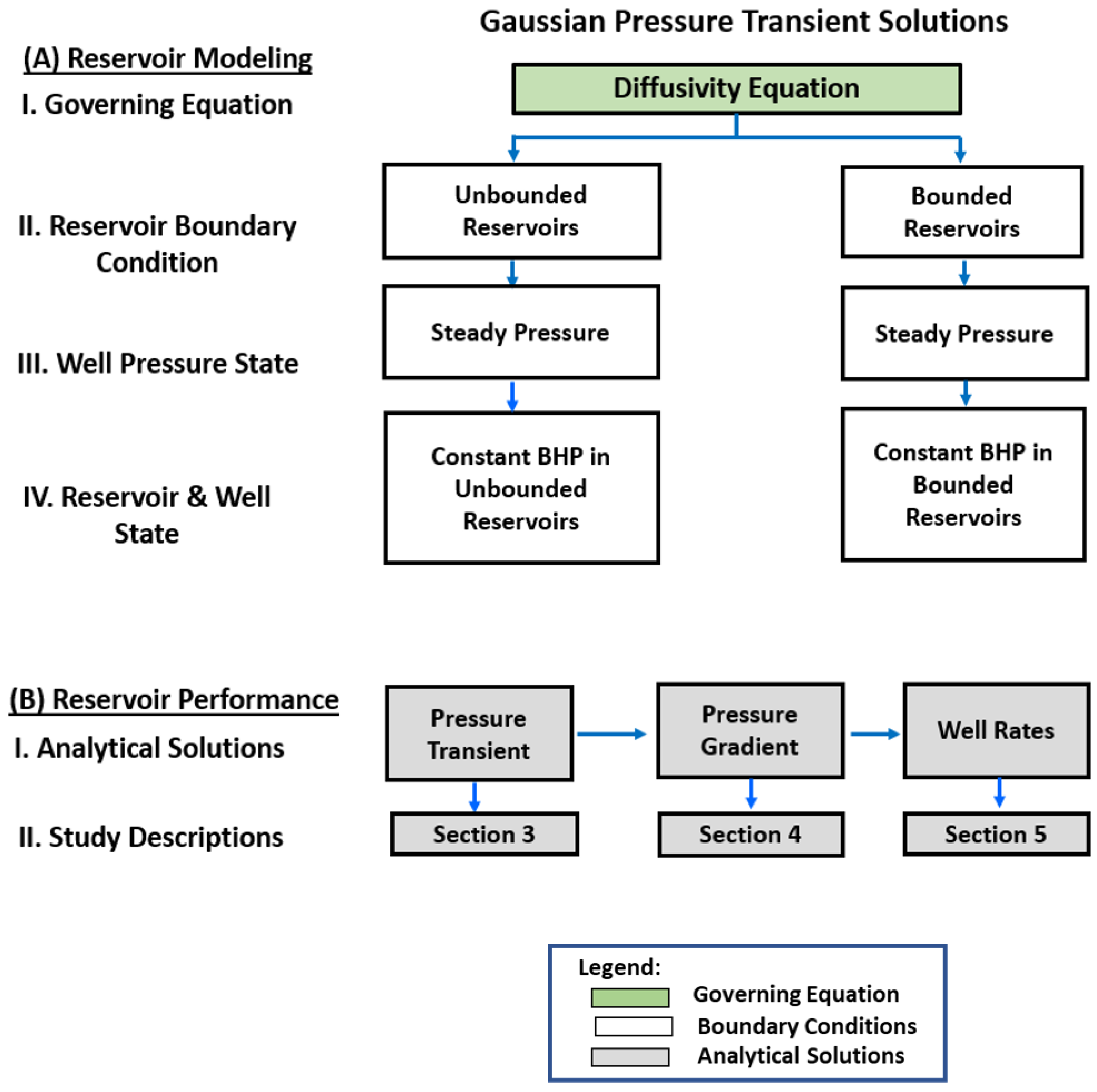
Figure 1 visually summarizes the key steps of our research workflow. It begins with the governing partial differential equation (PDE) that incorporates an hydraulic diffusivity term. Next, we show how reservoir and well boundary conditions are applied to this equation. The present study focuses on vertical wells in the transient-flow regime of reservoirs without lateral boundaries (unbounded) and with boundary-dominated flow effect [37]. Figure 1 illustrates how subsequent steps lead to the development of the proposed analytical solutions for well performance, starting from the transient pressure field solutions of the diffusivity equation. The pressure transient solutions in laterally unbounded reservoirs are provided in Section 3 of the present study.

Figure 1.
Summarized workflow for the mathematical model and application to either unbounded or bounded reservoirs produced with a vertical well.
3. Diffusion of Pressure Transients in Unbounded Reservoirs
This section focuses on pressure field solutions, which are the basis for the subsequent pressure gradient solutions’ development in Section 4, and is structured as follows. The classical diffusivity equation is revisited in Section 3.1. Many oil and gas wells are produced with artificial lift systems (using a pump) which impose a certain constant bottomhole pressure. Thus, the pressure transient diffusion solution is first derived for a constant bottomhole pressure change in vertical well systems in laterally unbounded reservoirs (Section 3.2). one- and two-dimensional pressure diffusion solutions are provided. We further distinguish between producer wells and injection wells.
3.1. Governing Diffusion Equation
Consider the classical diffusion equation [38], adapted for pressure diffusion in three-dimensional space:
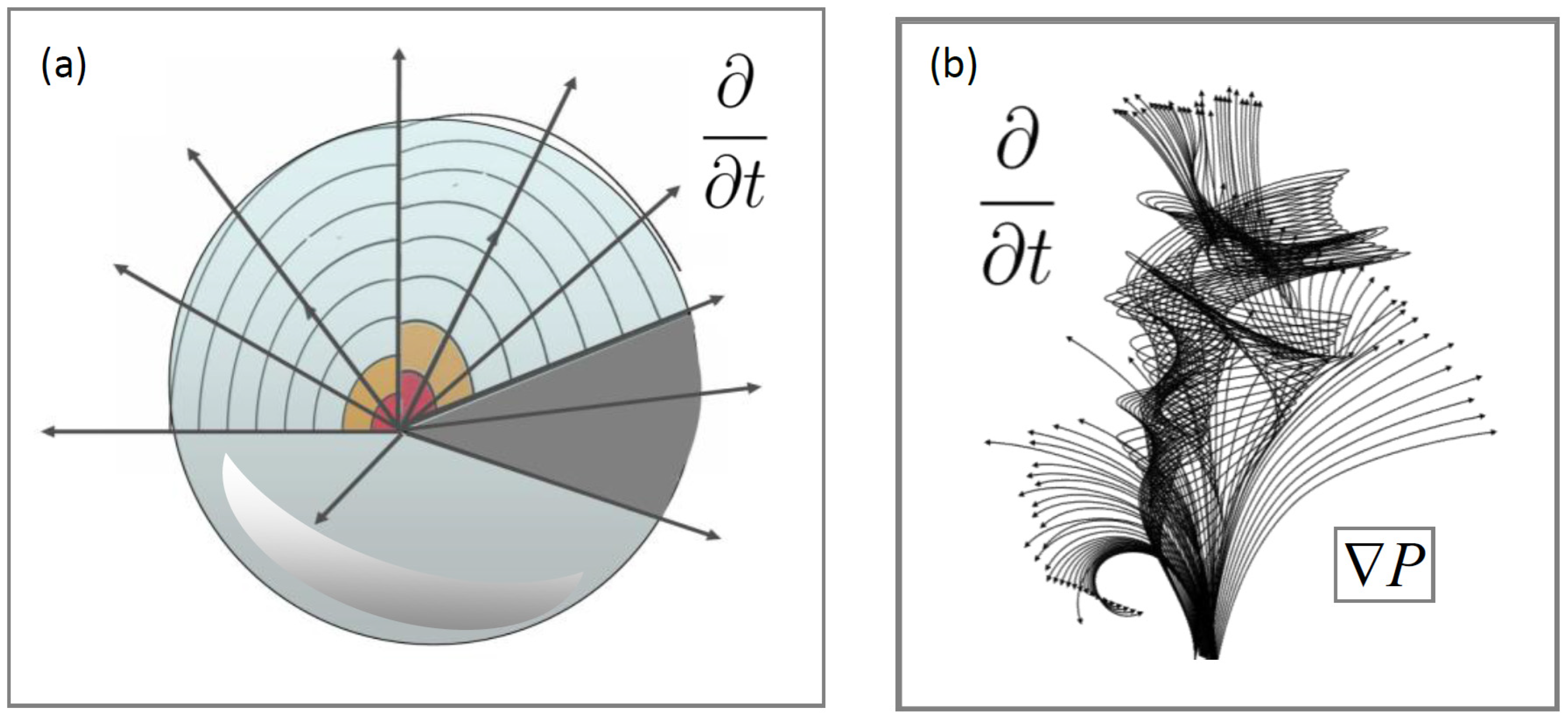
The first Del operator in Equation (8) takes the dot product or divergence of [MT−3], and denotes the pressure gradient. If normalized pressure is initiated at initial time, and gravity gradients are negligible, the spatial changes in are governed by Equation (8) as would apply to a perfectly homogenous, isotropic porous medium with slow, laminar flow due to the pressure gradient (Figure 2a).
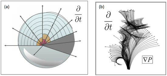
Figure 2.
Principle sketch of (a) 3D diffusion from a point source in a homogenous isotropic porous medium. (b) General 3D pressure diffusion process with inertia and consequently complex pressure transients.
For a free flow of liquid media, inertia and gravity force terms will quickly dominate the spatial changes in the pressure field, which is why the pressure gradients of free flow with turbulence may quickly appear extremely complex (Figure 2b). The pressure diffusion Equation (8) does not account for such additional terms. Also, only diffusion mass transfer due to the pressure gradient is considered. If molecular diffusion is included as well, the relative importance of the convective mass transfer due to the pressure gradient and that due to molecular diffusion can be described by a Fokker–Planck (convection–diffusion) equation [23,39]. A Gaussian Péclet number has been proposed to compare the relative importance of the two processes for application in gas reservoir/well dynamics [40].
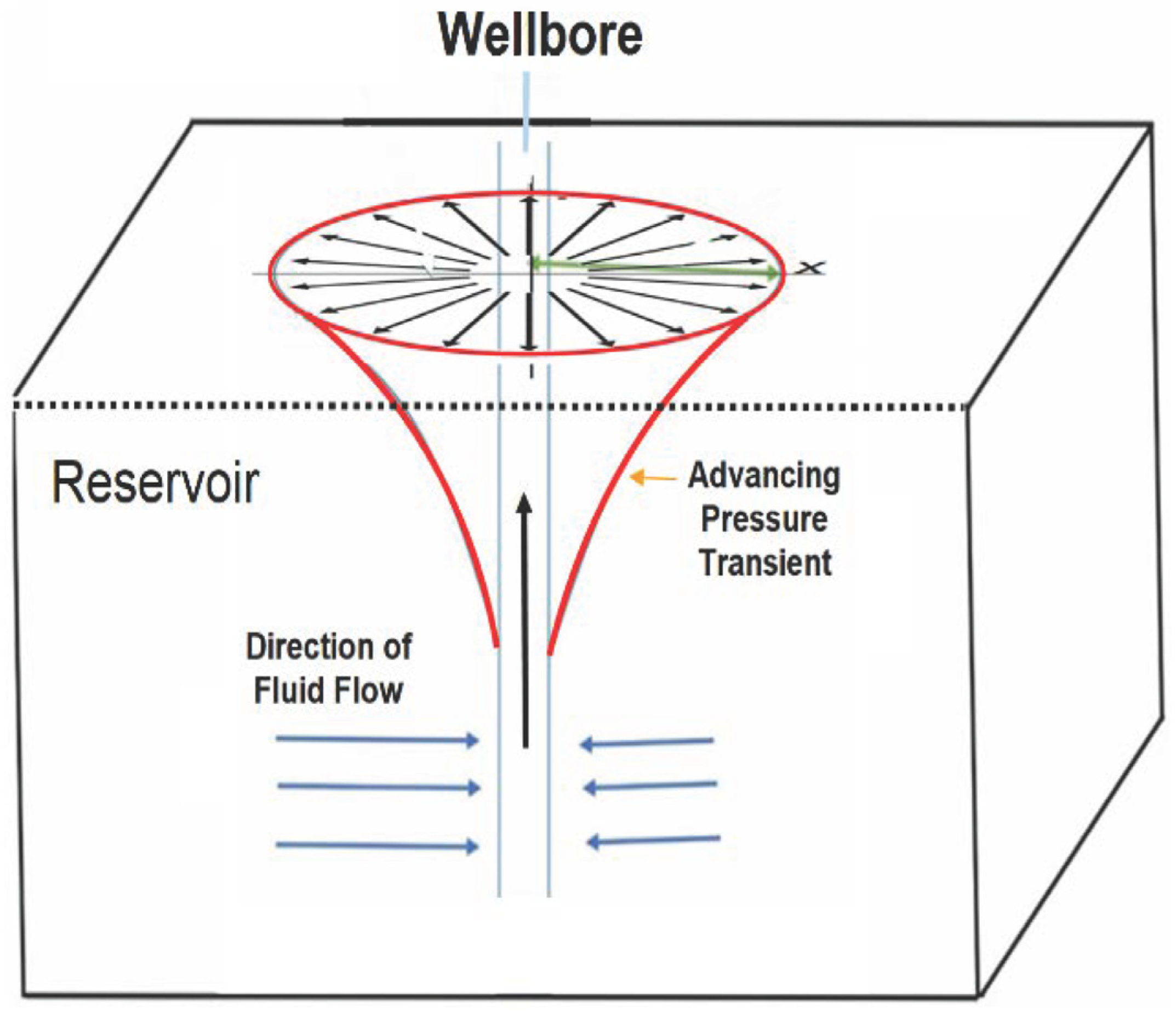
Next, assume the pressure diffusion process of interest occurs radially outward from a cylindrical well source placed vertically in a tabular homogeneous reservoir with an impervious upper and lower boundary (Figure 3) and at a certain initial pressure, . The pressure changes occur exclusively in the (x, y) plane, due to the no-flow condition at the upper and lower boundary. Specifically, 2D diffusion starting at the well is governed by:
where is modeled according to Zimmerman’s [18] hydraulic diffusivity equation (Equation (7)). The simplified PDE expression in Equation (9) is for an unbounded reservoir, meaning no lateral boundaries occur in the radial direction away from the well.

Figure 3.
Pressure transient advance (red) for the 2D diffusion of pressure perturbation initiated from a vertical well in a reservoir confined between impervious upper and lower boundaries, but laterally unbounded.
3.2. Steady Pressure Transient Diffusion (1D) for Production and Injection Wells in an Unbounded Reservoir
The key differences between injection and production wells are first established prior to presenting the solutions for such possible applications. Figure 4 illustrates a schematic of both types alongside their bottomhole pressures relative to the initial reservoir pressure. This helps visualize the distinct well designs used for injection and production purposes.
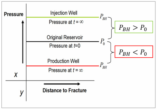
Figure 4.
Initial pressure (black line for t = 0) and final pressure states (green and red lines for t = ∞) in reservoirs for injection and production wells, respectively.
Injection wells: These wells have a higher bottomhole pressure than the original reservoir pressure. This pushes fluids outward away from the well landing point, following the pressure gradient, when injected into the formation.
Production wells: In contrast, production wells have a lower bottomhole pressure compared to the initial reservoir pressure. This pressure difference draws fluids inward towards the wellbore, enabling their extraction, and the drainage patterns enlarges as time goes.
For injection wells, we strive for a boundary condition where the injection pressure is initiated at with a value (Figure 4), and for t > 0, the source maintains a constant pressure differential , given by:
For production wells, the injection pressure is initiated at with a value (Figure 4), and for t > 0, the source maintains a constant pressure differential , given by:
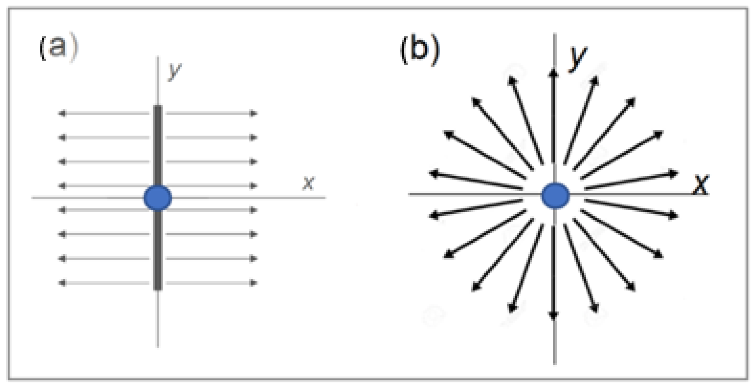
We also distinguish between well systems based on types of technical completion: wells drilled vertically and completed with a single longitudinal fracture (bi-wing fracture, Figure 5a) and those completed with simply a vertical, open-hole wellbore (Figure 5b). The bi-wing fractured wells are commonly used in low-permeability reservoirs; their pressure transient is governed by 1D diffusion from the fracture plane. The open wellbore without fracturing is used in high-permeability reservoirs; such wells act as 2D, cylindrical diffusion sources for the pressure transient. Studying the 1D and 2D cases jointly is instructive, in particular because we show in the present study how the 1D diffusion solution can be transformed to a 2D diffusion solution.

Figure 5.
Well types in map view. (a) Vertical well with bi-wing fracture acting as a 1D diffusion source. (b) Vertical well without fractures acting as a 2D diffusion source from the wellbore of radius .
3.3. Fractured Well Solution (1D Diffusion)
The pressure change component in the x-direction due to a planar, 1D diffusion source along the y-axis (Figure 5a) is as follows:
A valid 1D solution of Equation (12) with the boundary condition of Equation (10) was given by ([38], Equation 2.45):
Outside the well system, the pressure transient will change the reservoir pressure according to:
The time-dependent part of Equation (14) is given by Equation (13), which after normalizing gives the non-dimensional pressure change function [using for ] at any time and given position in the reservoir as follows.
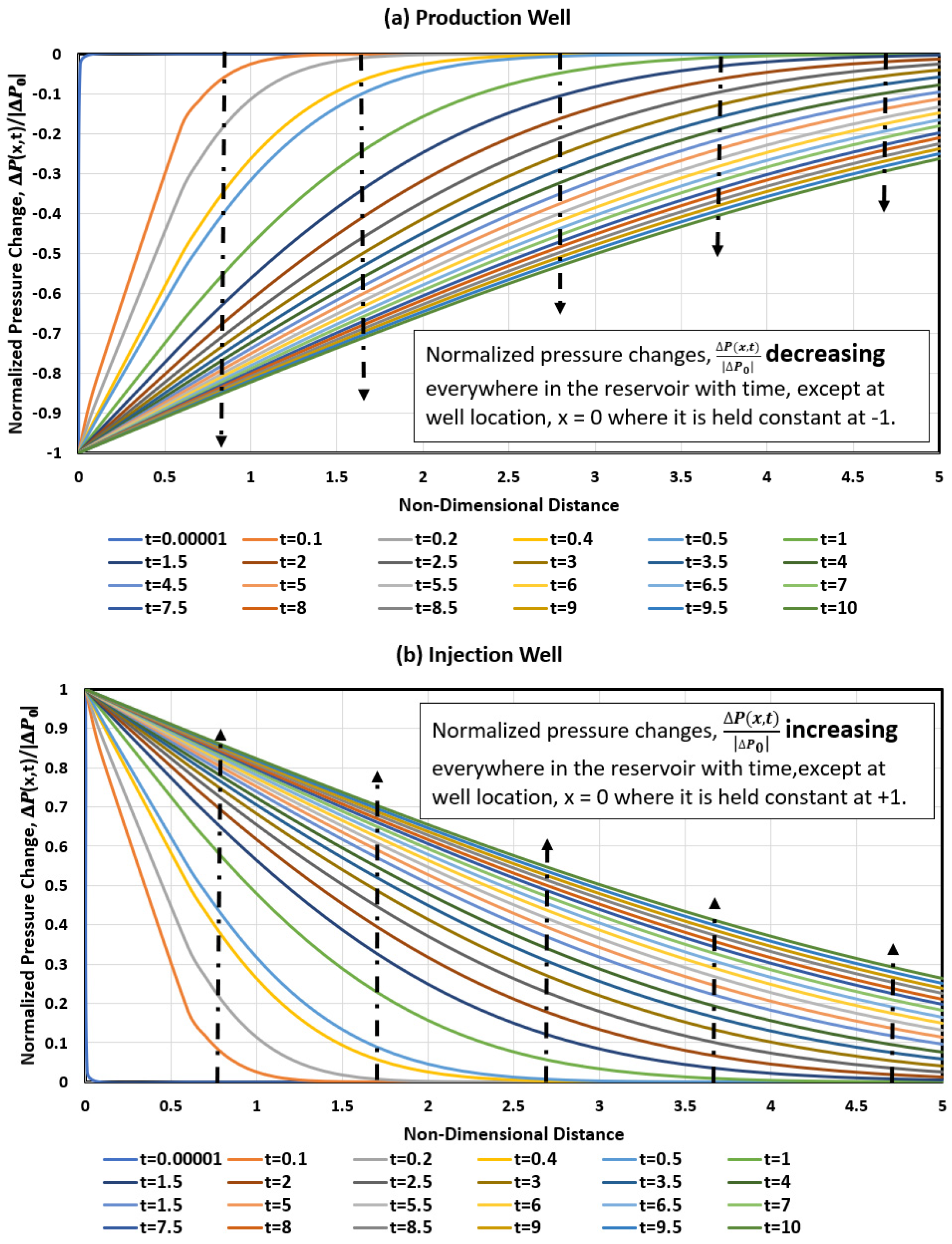
For the production well case, the initial reservoir pressure at the well location is changed by the well according to a step function, which lowers the pressure of the reservoir at with a value ; for 1D diffusion from a production well with a single fracture. The equation for the normalized pressure transient that travels perpendicular to the vertical fracture plane acting as the pressure change source is (Figure 6a):
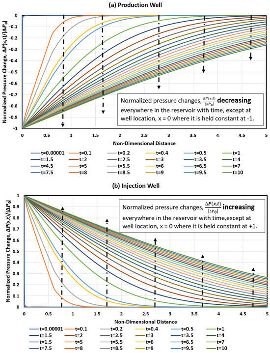
Figure 6.
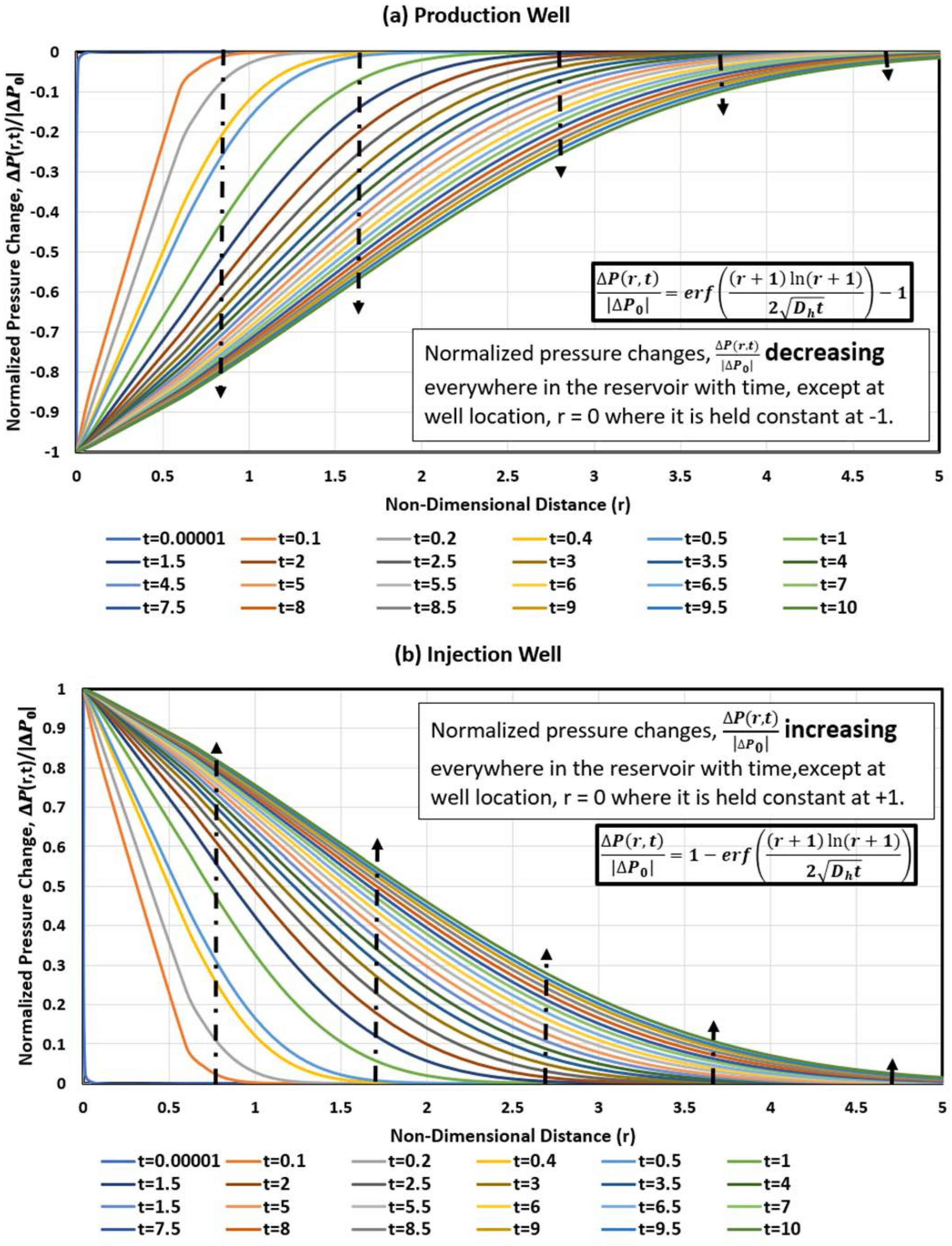
Normalized pressure changes for (a) 1D (planar fracture) production source shows pressure drawdown over time everywhere in the reservoir except at the fracture location (x = 0), where normalized pressure change is fixed at . (b) Injection well with constant scaled pressure change at the wellbore; = 1 shows how the pressure increases everywhere in the reservoir (from x = 0 to x = 5) as time increases from t = 0.00001 to t = 10 units of time. Diffusivity used: .
For a 1D diffusion from an injection source, the step function of the initial pressure increase in the well advances in the lateral reservoir space (x-direction) as follows (Figure 6b):
Figure 6a shows curves of the pressure transient progressively advancing across the reservoir space for time steps separated by 10 time units for the 1D diffusion of a hydraulically fractured production well, using Equation (15). The top border of the graph (y = 0) is where the original reservoir pressure, , remains unchanged. However, the non-dimensional pressure change initiated from the production well advances into the reservoir space and results in progressive pressure depletion associated with the fluid withdrawal process. Ultimately, after infinite time, the pressure everywhere in the reservoir will attain the bottomhole pressure, , which for the production case is given by the non-dimensional pressure change maximum at the bottom border of the graph (at y = −1) of Figure 6a.
Figure 6b shows the advance of the pressure change profiles at different times for the 1D diffusion of a fractured injection well, according to Equation (16). In this case, the bottom border of the graph (with y = 0) is where the original reservoir pressure, , remains unchanged. However, at a particular time, say t = 0.1 (depicted with yellow line in Figure 6b), the reservoir pressure has changed close to the wellbore, but asymptotically, no pressure change has occurred (yet) further away from the well. For the injector case, the pressures near the well location are increased, and the imposed pressure changes dissipate into the reservoir space as graphed in Figure 6b. Ultimately, after infinite time, the pressure everywhere in the reservoir will reach the bottomhole pressure, , which is given by the normalized pressure change top border of the graph (at y = 1) of Figure 6b.
3.4. Cylindrical Well Solution (2D Diffusion)
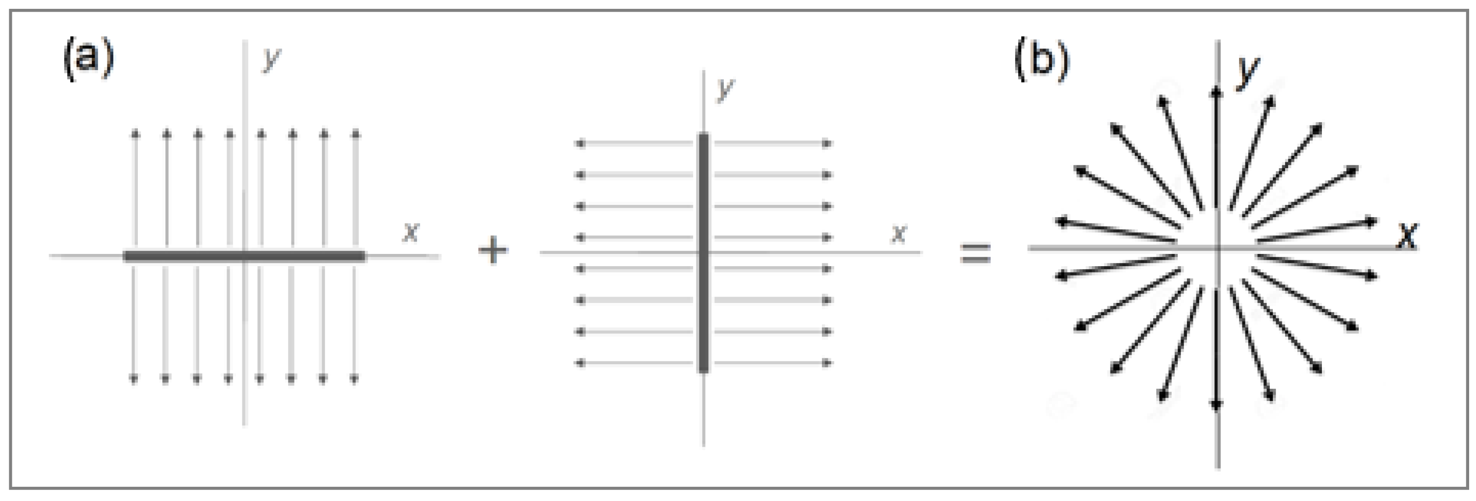
The advancing pressure change and normalized pressure depletion profiles for uni-directional 1D diffusion were given in Figure 6a,b. If we were to obtain the 2D solution (Figure 7b) by an orthogonal superposition of 1D pressure change sources (Figure 7a), it would give radial pressure gradients useful for flow path mapping. However, the rate of advance of the 2D diffusion process would be inaccurately scaled by the 1D diffusion process (as in Figure 6a,b), due to which the divergence of the flow paths and the required conservation of mass during the mass transport process will not be satisfied.

Figure 7.
(a) Superposition of two 1D diffusion sources in the origin to approximate a 2D diffusion source in (b), assuming the 1D sources along x and y are short finite lengths, such that they fit into a wellbore section of radius . It should be noted that such a superposition introduces a scaling error, as detailed in the main text. The conformal mapping of Figure 8 resolves this error.
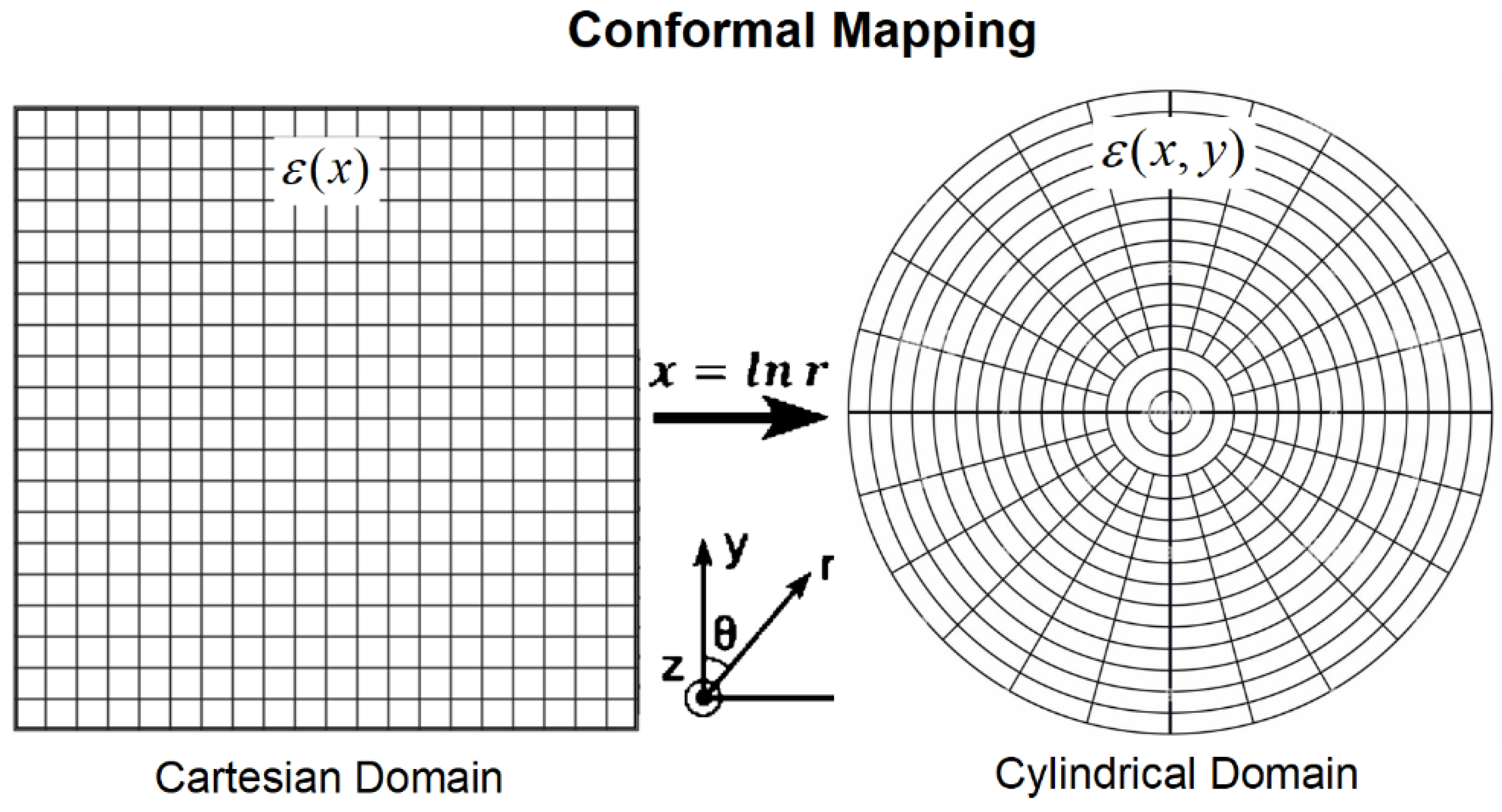
In order to correct for the divergence deficit, we apply a coordinate transformation of the 1D diffusion space to a 2D cylindrical diffusion space. The required transformation of the Cartesian reference system to a polar reference system can be achieved by conformal mapping (Figure 8), such that the normalized spatial coordinate x in domain ε(x) is mapped to lnr in the domain ε(x,y):
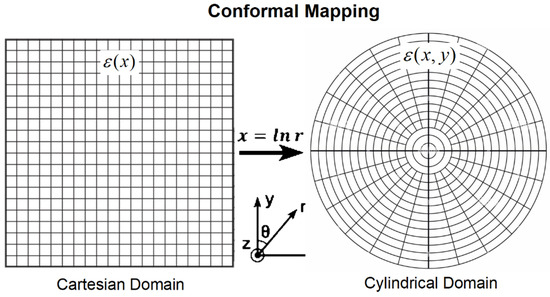
Figure 8.
Conformal mapping of the 1D diffusion solution in Cartesian space to divergent diffusion in radial directions by conformal mapping of coordinates from the ε(x) domain to the ε(x,y) domain.
For the production case, the solution of Equation (15) becomes (Figure 9a):
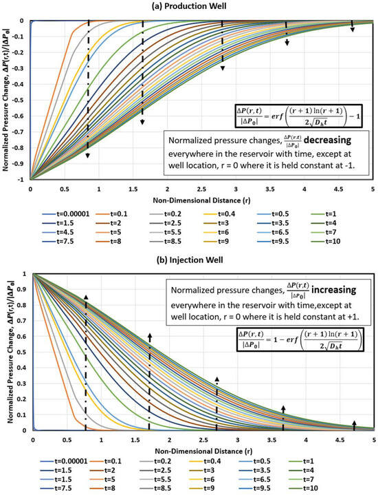
Figure 9.
Normalized pressure changes for (a) cylindrical pressure change source (such as occurs in the case of a production well) shows pressure-drawdown over time everywhere in the reservoir except at well location (x = 0), where normalized pressure change is fixed at −1. (b) Injection well with normalized pressure change at the wellbore, = 1.
For the injector case, the solution of Equation (16) becomes (Figure 9b):
It is important to note that the inclusion of “+1” in the numerator of Equations (18) and (19) serves to accurately represent the wellbore as a point source at r = 0. However, in practical wellbore applications, the spatial distance between the wellbore and the boundary typically precludes the necessity of this correction. To plot Figure 6a,b, no inputs are required other than normalized pressure change at the wellbore location and assuming a unit diffusivity. In Section 5, we will show how the well rate declines as a consequence of the lowered bottomhole pressure for a production well case with a specific dimensional hydraulic diffusivity. Unlike classical well test analysis, the well rate is not a boundary condition but an output of the applied bottomhole pressure, original reservoir pressure and hydraulic diffusivity (and well radius, which is assumed to be negligible in Figure 6a,b). The dimensional example of well rate computation and production forecasting using real field data from the early well life is included in Section 5.4.
Comparison of Figure 6a,b and Figure 9a,b reveals the slower advance of the pressure gradient due to the cylindrical source assumed as a consequence of the applied transformation.
Equations (18) and (19) are valid solutions of the general diffusivity equation in polar coordinates (Equation (20)):
4. Pressure Gradient Solutions
In Section 3, we focused on solving the pressure transient diffusion process from vertical sources (both injection and production wells with constant bottomhole pressures). We provided illustrative examples of how pressure changes will advance into the reservoir space away from a specific well location over time.
This section develops the solutions for the pressure gradients, which are of practical value for (1) plotting flow paths in the reservoir space and (2) computing the well rate. The flow paths can be identified as the local maxima of the pressure gradient solution (Section 4). Section 5 will explore the concept of well rate. Our objective here is to first present the pressure gradients for the unbounded reservoir solutions.
Flow in reservoirs is in each point principally controlled by the convective movement of mass along the direction of the local maximum of the pressure gradient. The diffusive mass transfer due to Brownian motion in the absence of pressure gradients is neglected in what follows, but if both pressure diffusion and molecular diffusion are considered, a Gaussian Péclet number has been proposed to compare the relative importance of the convective mass transfer due to the pressure gradient and that due to molecular diffusion [40].
4.1. Pressure Gradient Solution for 1D Diffusion
The gradient of the pressure change field for a 1D source (Equation (13)) in an unbounded reservoir is [using for ]:
The resulting pressure gradient in the radial direction away from a wellbore placed in the origin (depicted in the typical pressure diffusion configuration of sources Figure 5a,b), using a Cartesian grid for a 2D diffusion within the (x, y) plane, may be computed from the following equation, which gives the non-dimensional pressure gradient per length dimension [41]:
4.2. Pressure Gradient Solution for 2D Diffusion
To move from the pressure change solution of Equations (18) and (19) to the pressure gradient solution of the radial well for the injection case, we apply the derivative (Equation (23)):
Subsequently, the non-dimensional pressure gradient per unit length is (Equation (24)):
4.3. Comparison of 1D and 2D Pressure Gradient Solutions
Consider an injection well located at the center of the field of view, at (x, y) = (0, 0). Equations (22) and (24) describe the dimensionless pressure gradient solution per unit length of a 1D planar and a 2D cylindrical pressure source, respectively. The 1D pressure change solution of Equation (22) is here used to compare the pressure change advance from a well with two perpendicular sets of bi-wing fractures (short, with fraction of unit length) as in Figure 7b with the solution of the 2D-diffusion-driven flow around the cylindrical well as in Figure 8.
The resulting pressure gradient in the radial direction away from a wellbore placed in the origin (using a conjugate set of 1D planar sources as in Figure 5a,b), represented in a Cartesian grid for the resulting apparent 2D diffusion within the (x, y) plane, may be computed from [41]:
Substituting the 1D diffusion solution of Equation (22) into Equation (25) gives a Gaussian pressure transient solution for a vertical wellbore with two perpendicular, planar sources, using Cartesian coordinates (Equation (26)):
The non-dimensional pressure gradient per length dimension is (Equation (27)):
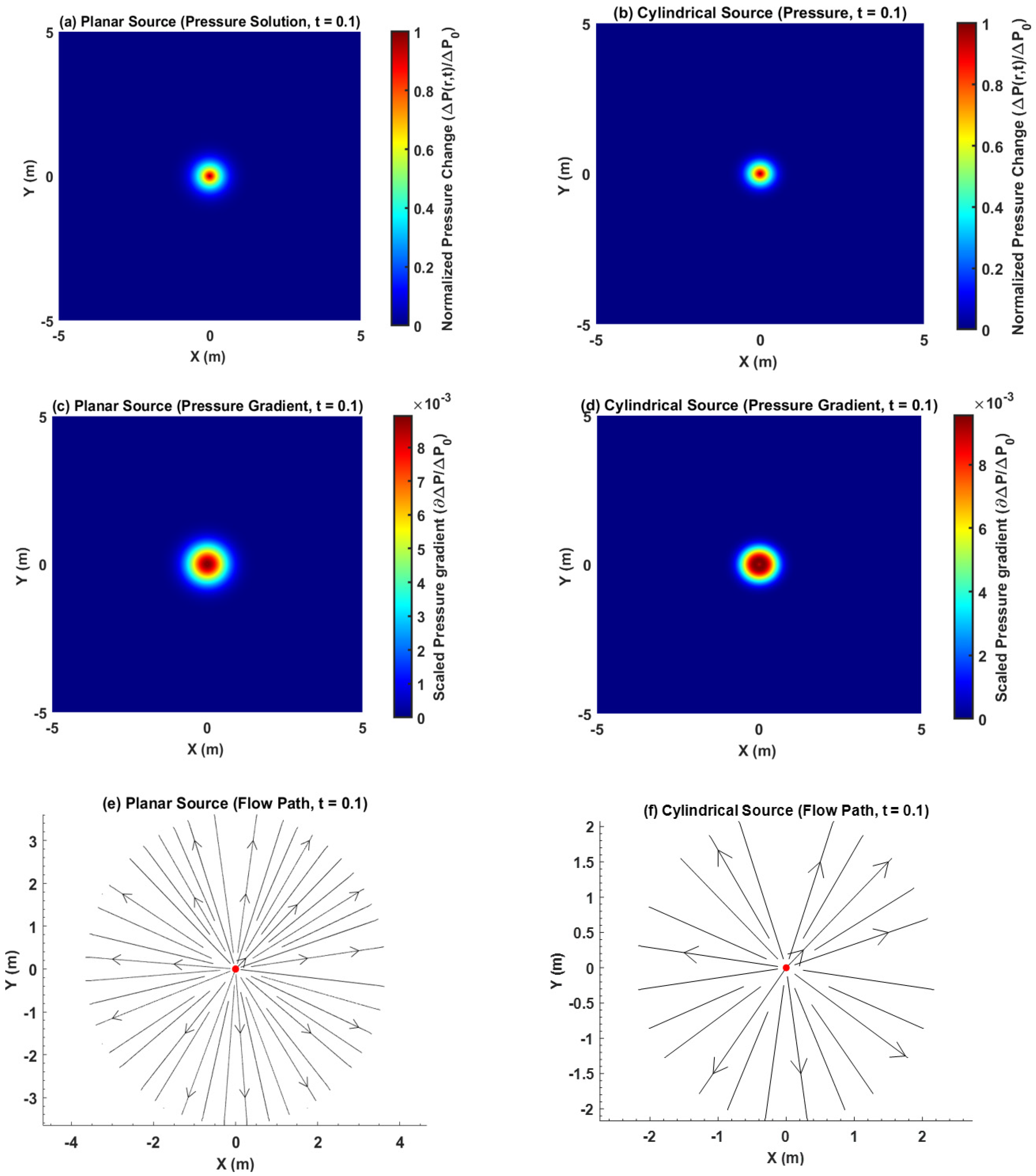
Figure 10a–f illustrates the early time development of the pressure fields, pressure gradients and flow paths for the 1D and 2D diffusion cases. The difference between the two cases for t = 0.1 remains modest.

Figure 10.
Contour maps for (a,b) normalized pressure change due to transient pressure diffusion, (c,d) pressure gradients and (e,f) flow paths, all at t = 0.1. The left column is for two orthogonal planar sources (a,c,e). The right column is for a cylindrical source (b,d,f).
We next re-examine the same two cases later in the well-life (Figure 11a–f), after considering t = 100, keeping input parameters the same, except that the field view dimension is increased from 5 to 50 units of spatial distance from the well location at r = 0. The difference between the two cases now becomes more pronounced. The arrows in Figure 10e,f and Figure 11e,f indicate the direction of fluid flow, which is radially outward for the injection well.
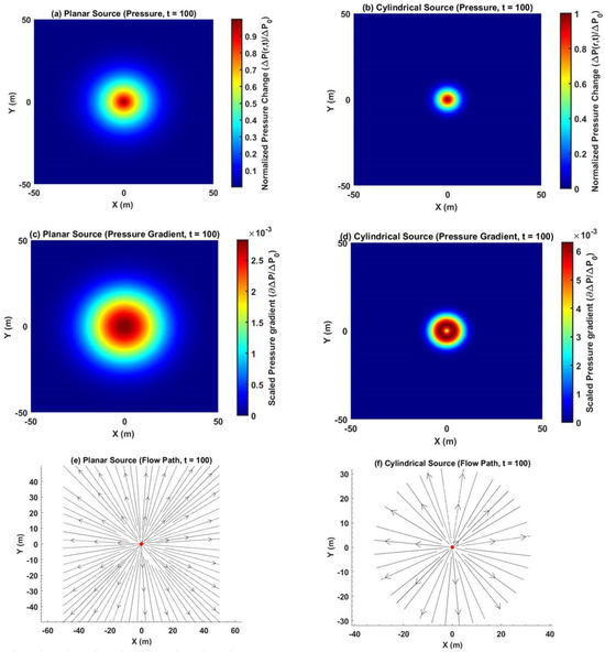
Figure 11.
Contour maps for normalized pressure change, pressure gradient and flow paths for two orthogonal planar sources (left column: a,c,e) and a cylindrical source (right column: b,d,f) at t = 100.
The purpose of computing the superposition of two orthogonal 1D planar diffusion sources (Figure 7 configuration) and the cylindrical 2D diffusion source obtained by the transformation of Figure 8 is to demonstrate the different outcomes. The correct procedure for a pressure transient initiated by a pressure disturbance at a cylindrical wellbore with a constant bottomhole pressure is to use the solution of Equation (24) not (27).
5. Well Rate Solutions
Building upon the foundation of pressure gradients laid out in Section 4, this section seeks to establish analytical solutions for well rates applicable to both injection and production wells.
5.1. Well Rate Solutions for Single Bi-Wing Fractured Well
The petroleum industry has shifted to massive use of horizontal wells that withdraw the fluid from ultra-low-permeability reservoirs via sets of transverse hydraulic fractures. Gaussian solutions for the 1D diffusion from such multi-stage fractured wells have been derived in recent companion studies [22,23,41,42,43,44,45]. The well rate solution for a fractured vertical well in a 2D Cartesian coordinate system is obtained using the time-dependent pressure gradient solution of Equation (21) for steady-state pressure diffusion in an unbounded reservoir in combination with Darcy’s Law. The pressure gradient accounts for the volumetric flow rate per unit cross-sectional area entering the fracture system of the well, using the relationship between flow rate and volumetric flow rate per unit fracture area, and , from Equation (3) to give the wellhead flow rate:
The factor 4 in the solution of Equation (28) stems from use of the fracture half-length and the fact that flow into the bi-wing fracture occurs from the reservoir space at either side of the fracture. The parameter accounts for the volume changes when fluid is lifted from reservoir space to the surface and is determined in specialized laboratories of sampled reservoir fluid in so-called PVT-analysis.
5.2. Well Rate Solutions for Cylindrical Wells in Laterally Unbounded Reservoirs
The solution for the rate of a vertical well is obtained using the time-dependent pressure gradient solution for steady-state pressure diffusion in unbounded reservoirs (Equation (23)). The volumetric flow rate per unit wellbore area, , was used to obtain the well rate, replacing r + 1 by ; assuming rw > 0:
The solution of Equation (29) differs from traditional well-testing equations of Equation (6). The latter assumes a constant well rate, which offers advantages for reservoir characterization using various well test rates at a constant imposed bottomhole pressure over brief periods of time, justifying treatment of both the bottomhole pressure and well rate as being approximately constant. However, it is possible to adapt our new solution for well test analysis [37]. Additionally, the future well rate can be predicted based on the pressure differential between the reservoir and the wellbore applied by the artificial lift system used.
5.3. Well Rate Solutions for Vertical Wells in Laterally Bounded Reservoirs
The solutions in the present paper so far are for vertical wells in transient flow due to a pressure drop originating from the well advancing into the ambient reservoir. The 2D diffusion is described with Gaussian pressure transients. While the research focus was initially on the production analysis of fractured wells used in so-called unconventional reservoirs (ultra-low-permeability rocks), the solutions offered in the present study are of equal practical significance for vertical injection wells and for vertical production wells in conventional formations. When the reservoir is at the lower end of the permeability spectrum, the transient flow period may last for much of the economic well life. Anisotropic diffusivity can be accounted for by using a hydraulic diffusivity tensor rather than scalar values. Examples have been given in Alotaibi et al. [35].
However, for conventional reservoirs with high permeability, the transient flow period will be limited to the early well life (first few months of production). To be of more practical value, the unbounded solution is expanded here in a solution for bounded reservoirs with an assumed cylindrical container shape of finite radius approximating the confined reservoir. Given that the Gaussian distribution relies on probabilistic concepts, a novel probability concept described in a prior study [46] was employed to formulate the innovative pressure diffusion model tailored for reservoirs dominated by bounded flow. To simulate the cylindrical reservoir boundary, the pressure front from the wellbore was superimposed, with a virtual pressure front originating from a cylindrical pressure source located at twice the distance between the well location,, and the effective reservoir boundary, (as elucidated in Figure A2, Appendix A of Afagwu and Weijermars [46]). The normalized pressure transient diffusion solution for laterally bounded cylindrical reservoirs for a production case is given as follows (Equation (30)):
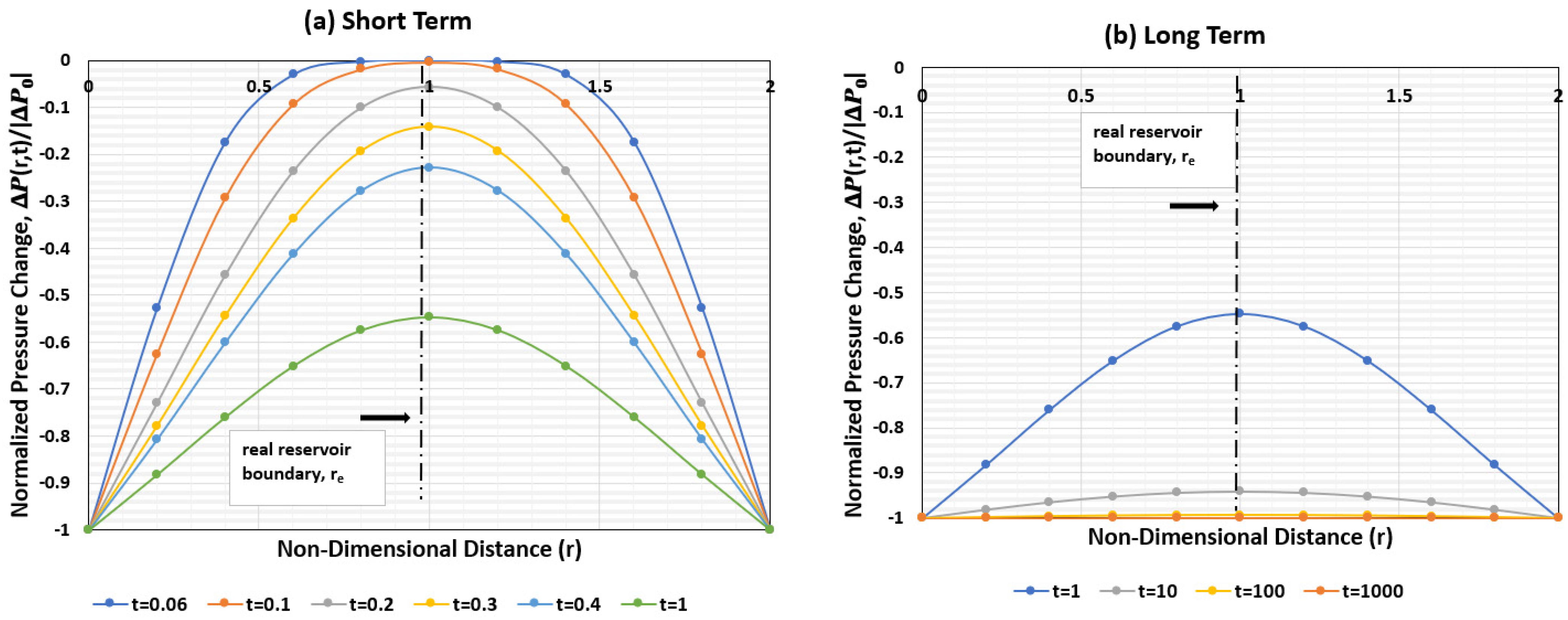
The validity of the normalized pressure solution (Equation (30)) is demonstrated in Figure 12 using the same approach originally described in our prior publication [46]. The tracked time-dependent pressure changes between the scaled wellbore location and real reservoir boundary confirmed that the boundary conditions were honored. The normalized pressure drawdown is at its maximum at the wellbore throughout the production period because of the constant bottomhole pressure boundary condition imposed at the wellbore. At the beginning, t = 0.06, there is no pressure change around the normalized real reservoir boundary, r = 1, (Figure 12a). However, from t = 0.1 units of time, there is gradual pressure change, suggesting that the pressure transient originating from the wellbore has reached the boundary. During late production time depicted by t = 1000 units of time, the pressure is nearly depleted everywhere in the reservoir (Figure 12b). Furthermore, the reduction in the steepness of the slope of spatial pressure changes indicates a corresponding decrease in gradient flux between the start of production at t = 0.06 units of time to late time, t = 1000.
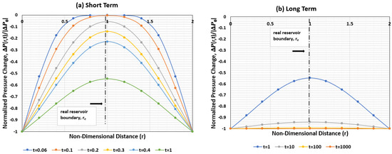
Figure 12.
Time-dependent normalized pressure change solution (Equation (30)) from the scaled wellbore position to the reservoir boundary extent, estimated with unit hydraulic diffusivity,. (a) Short unit of time, t = 0 to 1 unit; (b) longer period of production, from 1 to 1000 units of time.
The well rate expression of Equation (29) for the unbounded vertical well can now be modified as follows to account for the bounded reservoir case. The derivation of the wellbore flow rate solution for laterally bounded reservoirs follows the three-step procedure as follows: (1) Compute the time-independent pressure gradient solution for steady-state pressure diffusion in bounded reservoirs (Equation (30)). (2) Darcy’s Law integration: the pressure gradient is then integrated across the wellbore radius using Darcy’s Law (Equation (3)) to relate the pressure gradient to the volumetric flow rate per unit cross-sectional area entering the wellbore. (3) Wellbore flow rate relationship: the resulting expression is substituted into the relationship between flow rate and volumetric flow rate per unit area, , to give the wellbore flow rate model as follows (Equation (31)), where is the conversion factor from metric to field unit.
5.4. Application to Real Well Data
In this section, we give examples of history matching the production data from real wells with the GPT-based production forecasting method. In prior studies, partial solutions were compared with results from numerical simulators with excellent matches [37,41]. In the present study, we use real production data to demonstrate the value of our new solutions in practical applications. The production data for our chosen study wells come from decommissioned UK offshore fields, which have been made publicly available by the UK North Sea Transition Authority, as was detailed in [47].
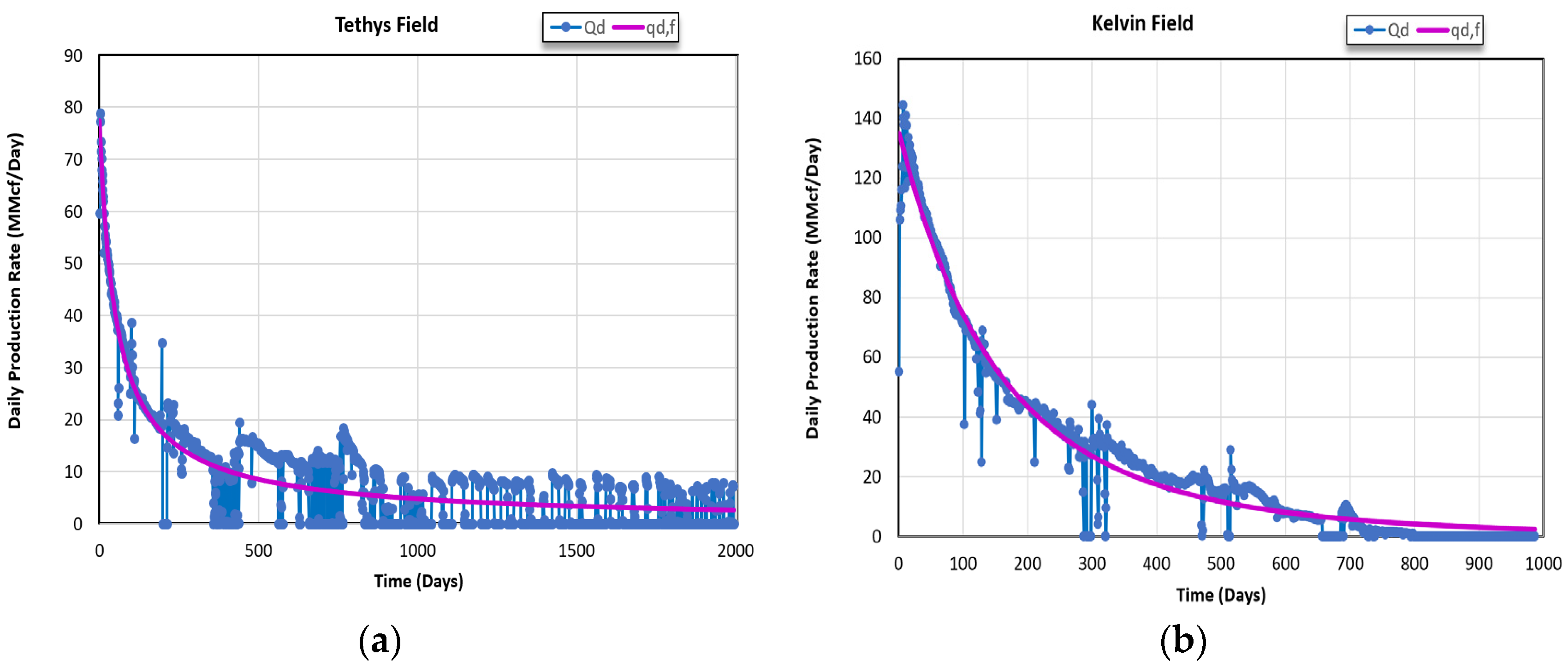
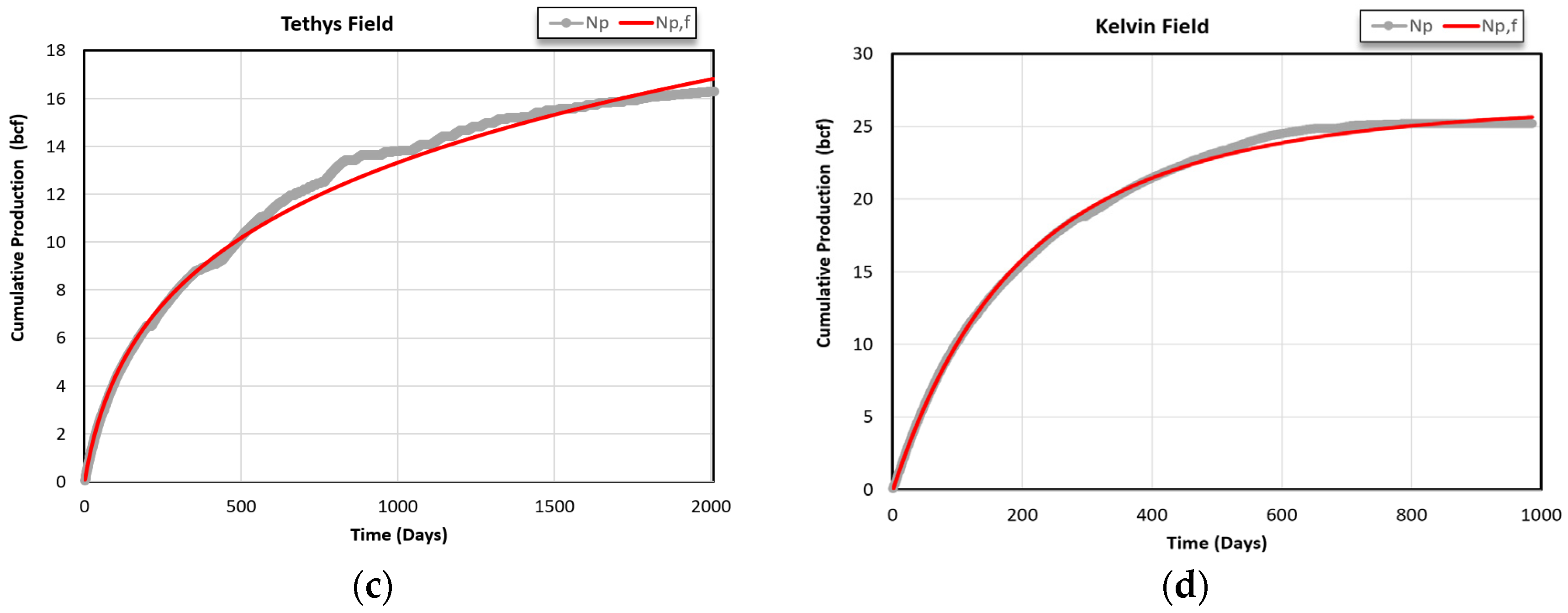
The daily production data and cumulative production data of study wells from two UK offshore gas fields (Tethys and Kelvin) are plotted in Figure 13a–d. The Tethys field occurs in rocks of Permian age: the Leman Sandstone Formation of the Lower Permian Rotliegendes Group [47]. The Kelvin field is hosted in fluvial sandstones of the Upper Devonian–Carboniferous Fairway. When the full field data are used, it appeared in our prior study that use of the empirical decline curve analysis (DCA) method by Arps to historically match the production data can give curve matches that closely match the actual well behavior (Figure 13a–d).


Figure 13.
Daily production rates (top row, (a,b)) and cumulative production (bottom row, (c,d)) of the Tethys and Kelvin Wells were fitted with Arps DCA curves [47] and provided excellent history matches throughout the well life. The detailed fitting parameters are given in [47].
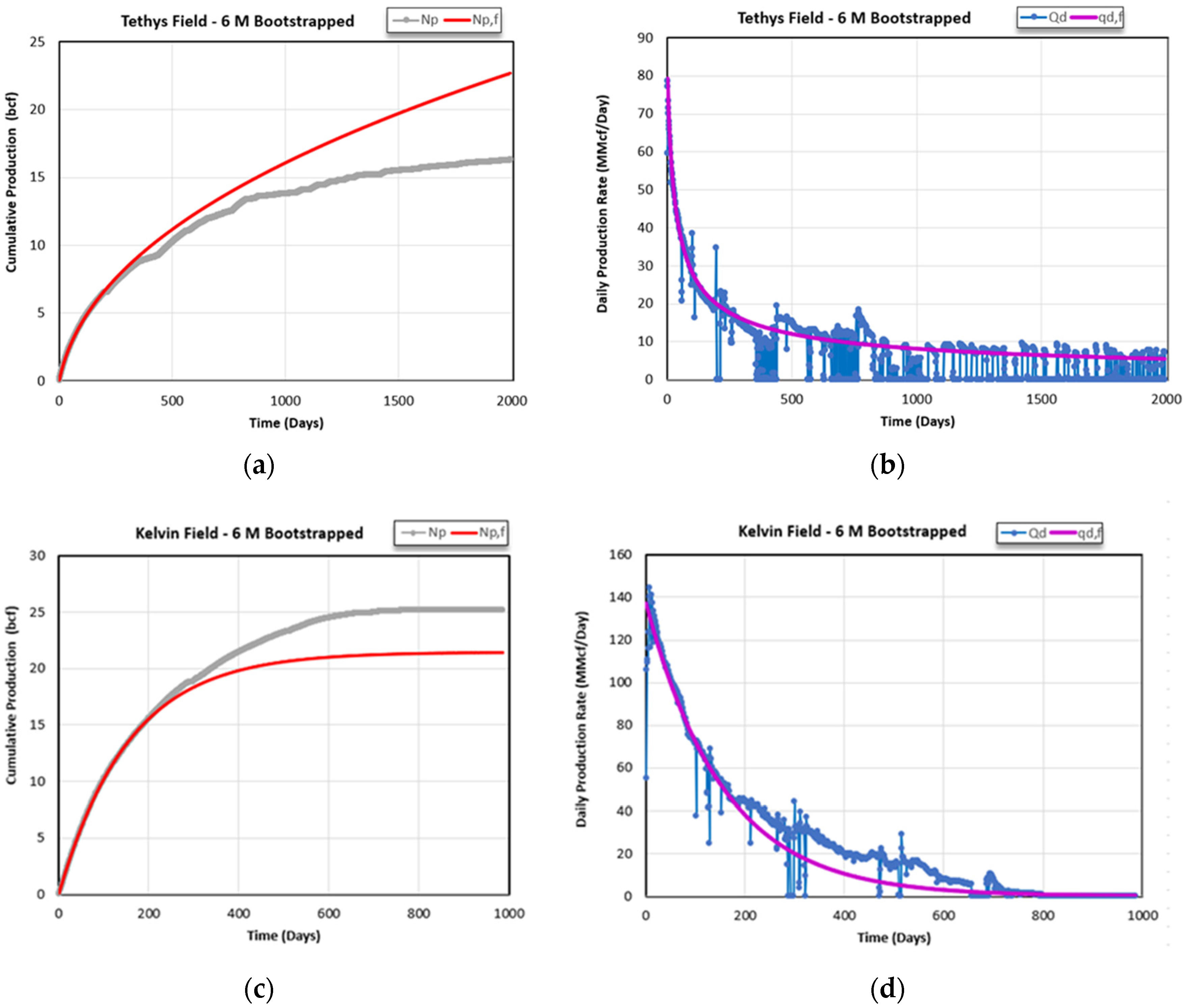
However, for production forecasting of newly drilled wells and establishing the estimated ultimate recovery (EUR) volumes for reserve estimation, only a few months’ production data would typically be available. We therefore tested how well Arps forecast the actual well behavior, if we used only the first 6 months of bootstrapped daily production data [47]. It then appeared that the Arps method gave rather inaccurate forward prediction of the well rates and either overestimated (Tethys) or underestimated (Kelvin) the ultimate recovery (EUR) volumes (Figure 14a–d).
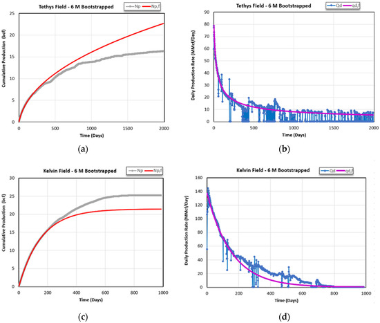
Figure 14.
History matching of full well-life cumulative production and daily rates using only the first 6 months of daily production [47] gave poor history matches for the post-6-month production behavior for both the Tethys Well (top (a,b)) and the Kelvin Well (bottom (c,d)). The detailed fitting parameters are given in [47].
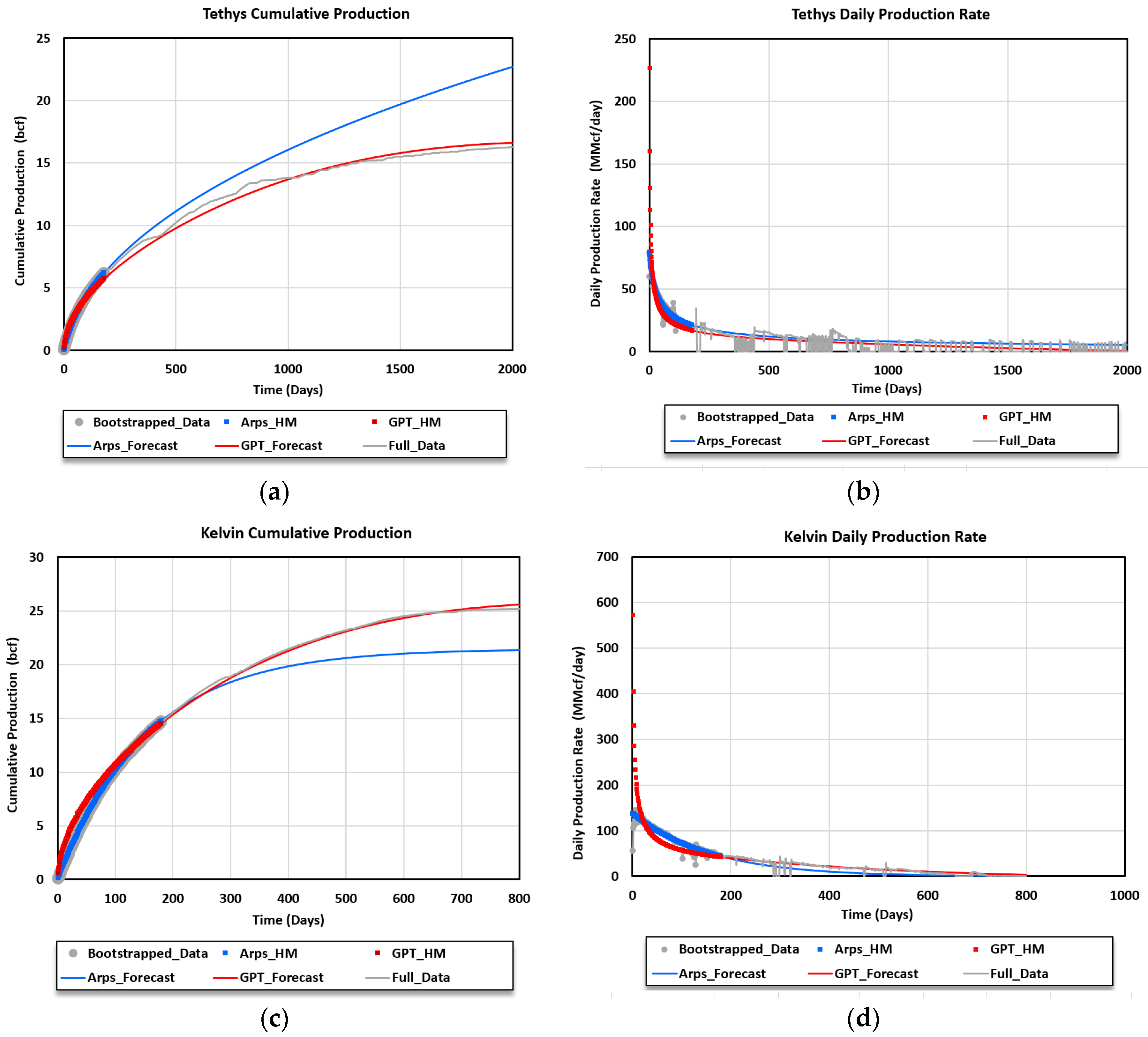
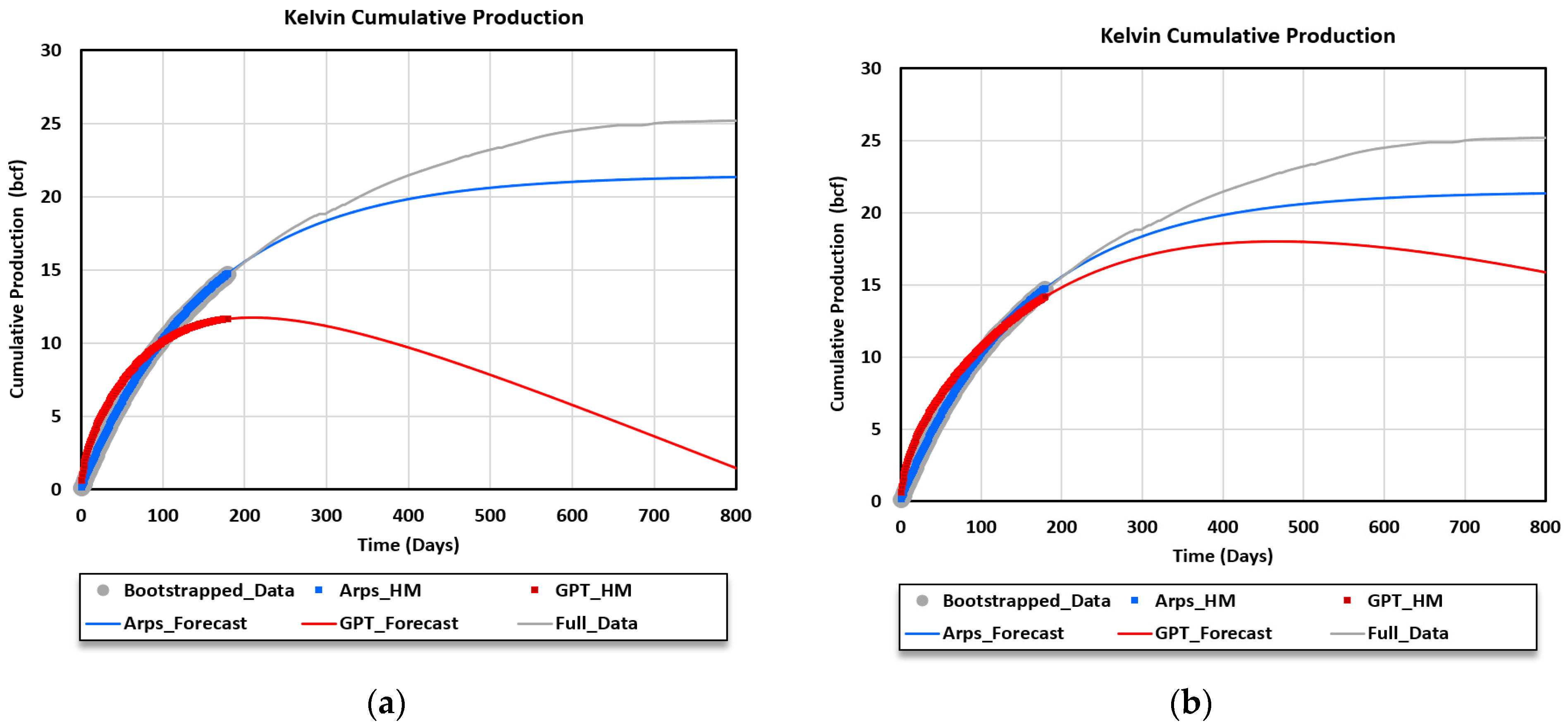
The conclusion was that the empirical Arps method becomes increasingly inaccurate when only a few months of production data are available. Remedying this limitation was one of the motivations to develop our physics-based GPT history-matching solution. The bounded solution of Equation (31) was incorporated in a spreadsheet for history matching the early production data, together with the traditional Arps equation described in [47], to check how well the physics-based GPT history match will predict the future well performance and EUR if again only the first 6 months of the historic production data were used. Figure 15a–d gives the outcome of the least square error history matches for both the Arps DCA and the GPT methods. Our conclusion is that using the physics-based GPT solution for a bounded reservoir gives excellent history matches. The detailed fitting parameters used in Equation (31) are given in Table 1.
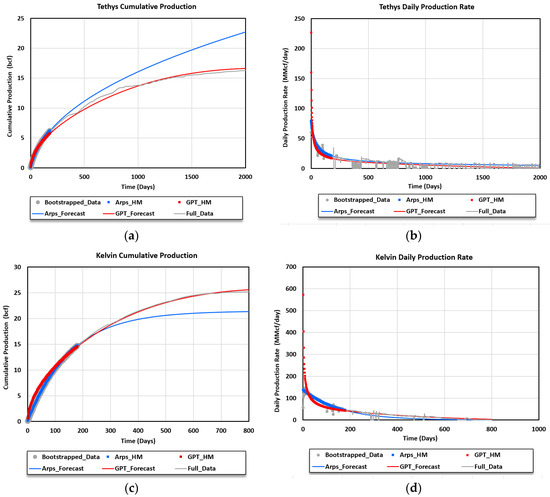
Figure 15.
History matching of full well life cumulative production and daily rates using only the first 6 months of daily production [using the GPT solution-method, Equation (31) (red curves) gave excellent history matches for the post-6-month production behavior (gray curves) for both the Tethys Well (top (a,b)) and the Kelvin Well (bottom (c,d)]. The detailed fitting parameters are given in Table 1.

Table 1.
GPT fitting parameters used for Figure 15 results.
Apart from the excellent history matches obtained with GPT, an additional strength is its diagnostic value for reservoir characterization. For example, the effective radius of the reservoir is obtained from the history-matching process (last row in Table 1). Once the effective radius has been determined in the history match, changing the reservoir radius parameter shows how the transition from transient flow to boundary dominated flow would shift. For example, if the radius of Kelvin reservoir reduces from 5500 to 2750 ft, the boundary-dominated flow occurs much earlier, and the reservoir would effectively be depleted after 200 days (Figure 16a). If we use a 4000 ft radius, the reservoir would deplete after 450 days (Figure 16b). Because the well is known to produce for 800 days, the physics-based GPT model correctly shows a larger reservoir radius of 5500 ft.
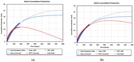
Figure 16.
Sensitivity of GPT solution, Equation (31), to reservoir radius. (a) Radius reduced to half of the history-matched value of 5500 ft (Table 1); the EUR would reduce from 25.8 to 12.2 bcf. (b) Radius reduced from 5500 ft to 4000 ft shrinks the productive well life from 800 to 450 days; the EUR would reduce from 25.8 to 18 bcf.
5.5. Further Applications of Pressure-Transient-Based Well Rate Solutions
The pressure-transient-based well rate solutions can be used in a variety of practical applications:
- Pressure transient simulation: These solutions can simulate the pressure transients caused by fluid flow towards a well system in unbounded and boundary-dominated flow reservoirs. Such solutions allow for analyzing the dynamic behavior of pressure during production or injection (see Figure 6 and Figure 9).
- Reservoir petrophysical characterization: By analyzing well test data using these solutions, reservoir properties can be characterized [37], such as:
- Permeability (k): A key parameter controlling fluid flow in the reservoir.
- Skin factor: A dimensionless parameter that quantifies wellbore damage (positive skin) or stimulation (negative skin).
- Effective wellbore radius (which includes skin factor): This reflects the actual flow area around the wellbore, potentially influenced by formation damage or stimulation.
- Field development planning: By integrating the information obtained from well test analysis (permeability, skin factor and transient distance), these solutions can guide investment decisions for field development. This can help ensure the reservoir meets stakeholder expectations by selecting an appropriate development plan based on exploratory and appraisal well data.
6. Discussion
6.1. Importance of Well Rate Forecasting Methods
Accurate production forecasts and reserve estimations are particularly important for the global petroleum industry in order for individual companies to estimate their remaining hydrocarbon reserves which underpin the book value of their fixed assets in the balance sheet and serves as collateral for credit lines. Reporting of the proved reserves (P90 certainty) is mandatory as per the guidelines of the US Security and Exchange Commission (SEC) and applies to all petroleum companies listed on the New York Stock Exchange (NYSE).
Two types of practical tools for well rate forecasting are widely used.
One type of tool is the commercial reservoir simulators (GMC, Kappa, Eclipse, etc.), of which many different varieties are offered by service companies, which provide slick interfaces with ready-to-use input boxes. The actual computations are invariably based on numerical, finite difference computational solution methods. While the results are reasonably accurate, the user licenses for the commercial simulators are costly, the methods and assumptions involved are non-transparent and filling out the detailed well data in the user interface requires quite a bit of practical experience. Also, the runtime to obtain output may take several hours, especially when probabilistic determination of reserve categories is required.
The other principal type of tools popular for determining hydrocarbon well performance and related reserves reporting is based on empirical decline curve analysis. Numerous decline curve analysis (DCA) formulas have been proposed in the past, as reviewed in considerable detail elsewhere [48,49]. These tools are not physics-based and largely phenomenological and use real well data to match decline curve formulas and then project the future well performance based on the historic trend. Analogy and type-curve well assumptions are extensively used to book reserves based on still undrilled but vacant well locations in the acreage leased by the companies.
The solutions for well rate forecasting for fractured wells (Equation (28)) and cylindrical wells (Equation (29)) in unbounded reservoirs and vertical wells in bounded reservoirs (Equation (31)) provide physics-based analytical solutions to predict well performance. The key unknown parameter for new reservoirs to be drilled is the hydraulic diffusivity. The diffusivity can be computed either using Equation (7) with primary parameter inputs, or by history matching early pilot well data, as demonstrated in [50].
Table 2 lists the strengths and weaknesses of the existing types of tools for well analysis, production forecasting and reserve estimation. Because nodal analysis is rather technical and requires specialist knowledge, companies apply the tool only sparsely. Strengths and weaknesses of the new Gaussian pressure transient solution are also included. A major strength of the Gaussian method is that historic well data are not needed to predict the performance of a new well, provided the hydraulic diffusivity is already known from applying Zimmerman’s Equation (7).
Table 2.
Strengths and weaknesses of various production analysis tools.
6.2. Relation to Prior Work
In previous research, various analytical solutions have been devised for interpreting well testing data and calculating well rates resulting from pressure changes induced by production in aquifers and oil reservoirs [17,18,20,21]. However, these earlier solutions typically assumed a constant well rate as the boundary condition. This assumption does not align with real-world scenarios where fluid withdrawal or injection is managed by pump devices that maintain a constant bottomhole pressure, a common practice in oil and gas wells equipped with artificial lift systems. Consequently, the ability to rapidly compute the decline and associated changes in the well rate over time based on the pressure differential applied at the well by the lift system (pump) relative to initial reservoir conditions has been constrained by the absence of concise expressions accommodating the constant bottomhole pressure boundary conditions.
The present study refined and expanded upon the analytical solutions established in recent works [22,42]. The earlier contributions provided valuable insights into fluid dynamics within subsurface reservoirs and introduced initial techniques for analytical modeling to compute well rates based on hydraulic diffusivity derived from real field data and production-induced pressure changes, with a particular emphasis on unconventional reservoirs.
By introducing a new analytical solution that accommodates constant bottomhole pressure boundary conditions and incorporates pressure interference from neighboring wells or external boundaries through the superposition of a cylindrical image source, the present study represents a significant leap forward from prior work. This advancement bridges the gap between theoretical models and practical applications by offering a practical and efficient approach for analyzing well testing data and computing well rate changes under constant bottomhole pressure conditions. Moreover, the new solution eliminates the need for time-intensive pressure-matching procedures, such as nodal analysis, for determining well rate declines in systems operating under constant bottomhole pressures. Through a reassessment of the diffusivity equation and the derivation of tailored well rate equations, this study provides a practical and efficient means to compute well rate changes based on fundamental physical parameters, while also accounting for pressure interference effects on diffusion and offering insights into the sensitivity of engineering parameters to outcomes.
The following practical recommendations can be formulated based on the insights from this study:
- Analyze real-world historical reservoir pressure and production measurements with instantaneous and steady pressure analytical solutions. Refer to well test paper success in providing valuable estimates of parameters relevant for modeling real-world reservoir behavior.
- Expanding analytical models to incorporate multi-phase flow phenomena, such as gas–liquid interactions or phase behavior effects, would advance our understanding of complex reservoir systems and enable more accurate predictions of production rates.
- Explore methods for incorporating uncertainty analysis into analytical models, allowing for probabilistic assessments of reservoir performance and providing decision-makers with more robust risk assessments.
- Explore the application of analytical models to emerging reservoir types, such as geothermal reservoirs, to expand the scope of their applicability and address pressing challenges in energy production.
- Conduct comparative studies to validate the evolving analytical models and benchmark their performance against empirical data to enhance confidence in their predictive capabilities and facilitate their adoption in practical engineering applications.
These recommendations represent potential avenues for further research aimed at advancing our understanding of reservoir behavior and improving the effectiveness of reservoir management practices. By addressing these research areas, we can meaningfully contribute to the sustainable development of energy resources and the optimization of reservoir performance.
7. Conclusions
This study introduces novel analytical solutions for computing well rates in aquifers and oil reservoirs under the condition of constant bottomhole pressure, a scenario often encountered in practical applications involving pump devices, addressing a significant gap in the prior literature. Previous solutions assumed a constant well rate. The new solutions presented in this study enhance the understanding of system dynamics and ensure the precision of production metric estimations. This represents a significant step forward in the field of analytical modeling for well testing and reservoir management. This new approach enables the rapid computation of well rate changes based on pressure differences, reservoir permeability, diffusivity and fluid properties. This study derives a solution for the pressure diffusion equation with a constant bottomhole pressure boundary condition, allowing for the computation of well rate changes without the need for elaborate time-stepped procedures.
Our research builds upon the foundation laid by previous works, as evidenced by the contributions of the Weijermars research group [22,23,42]. The emphasis in the present study is on applying the diffusion equation to a vertical wellbore in a horizontal, permeable reservoir, assuming a constant bottomhole pressure. Furthermore, our approach provides a comprehensive framework for understanding reservoir dynamics and optimizing production strategies.
The discussion section highlights the advantages of the proposed solution over nodal analysis, a traditional method for computing declining well rates. The new solution eliminates the need for time-stepped pressure matching and provides a more straightforward and rapid approach for forecasting well rates. The paper also compares the new solution to other forecasting tools, such as reservoir simulators, decline curve analysis and nodal analysis, outlining the strengths and weaknesses of each approach. The derived Gaussian pressure transient solutions offer practical benefits, particularly for wells produced with artificial lift systems, and provide a valuable alternative and complement to existing methods used in the petroleum industry. In conclusion, our study represents a significant advancement in the field of reservoir engineering, offering a robust analytical toolkit for estimating well rates and paving the way for more accurate and efficient reservoir management in the oil and gas industry.
Author Contributions
Conceptualization, R.W.; methodology, C.A.; software, C.A.; validation, R.W. and C.A.; formal analysis, R.W. and C.A.; investigation, R.W. and C.A.; data curation, R.W.; writing—original draft, R.W.; writing—review and editing, C.A.; visualization, R.W. and C.A. All authors have read and agreed to the published version of the manuscript.
Funding
The APC was funded by the College of Petroleum Engineering & Geosciences (CPG) at King Fahd University of Petroleum & Minerals (KFUPM).
Data Availability Statement
The data presented in this study are available from the UK North Sea Transition Authority.
Acknowledgments
The authors acknowledge the generous support provided by the College of Petroleum Engineering & Geosciences (CPG) at King Fahd University of Petroleum & Minerals (KFUPM).
Conflicts of Interest
The authors declare no conflict of interest.
Correction Statement
This article has been republished with minor corrections to resolve the typographical errors. The corrections include updates to Equations (20) and (23). These changes do not affect the scientific content of the article.
Nomenclature
Nomenclature is provided with units in metric and field units in parentheses.
| ( | ||
| (ft) | ||
| (ft) | ||
| (ft) | ||
| (ft/day) | ||
| (ft/day) | ||
| (scf/day) | ||
| (ft) | ||
| (ft) | ||
| (day) | ||
| ( | ||
| (ft/day) | ||
| (ft) | ||
| (psi/ft) | ||
| (1/ft) | ||
References
- Matos, C.R.; Carneiro, J.F.; Silva, P.P. Overview of Large-Scale Underground Energy Storage Technologies for Integration of Renewable Energies and Criteria for Reservoir Identification. J. Energy Storage 2019, 21, 241–258. [Google Scholar] [CrossRef]
- Stober, I.; Bucher, K. Geothermal Energy; Springer International Publishing: Cham, Switzerland, 2021. [Google Scholar] [CrossRef]
- Olah, G.A.; Goeppert, A.; Prakash, G.K.S. Beyond Oil and Gas: The Methanol Economy; Wiley: Hoboken, NJ, USA, 2009. [Google Scholar] [CrossRef]
- Quaschning, V. Renewable Energy and Climate Change; Wiley: Hoboken, NJ, USA, 2010. [Google Scholar] [CrossRef]
- Ajayi, T.; Gomes, J.S.; Bera, A. A review of CO2 storage in geological formations emphasizing modeling, monitoring and capacity estimation approaches. Pet. Sci. 2019, 16, 1028–1063. [Google Scholar] [CrossRef]
- Berkowitz, B. Characterizing flow and transport in fractured geological media: A review. Adv. Water Resour. 2002, 25, 861–884. [Google Scholar] [CrossRef]
- Hesse, M.A.; Tchelepi, H.A.; Orr, F.M. Scaling Analysis of the Migration of CO2 in Saline Aquifers. In Proceedings of the SPE Annual Technical Conference and Exhibition, San Antonio, TX, USA, 17–20 September 2006. [Google Scholar] [CrossRef]
- Fourier, J.B.J. Theorie Analytique de la Chaleur; Didot: Paris, France, 1822; pp. 499–508. [Google Scholar]
- Fick, A.V. On liquid diffusion. London, Edinburgh, Dublin Philos. Mag. J. Sci. 1855, 10, 30–39. [Google Scholar] [CrossRef]
- Darcy, H. Les Fontaines Publiques de la ville de Dijon: Exposition et Application des Principes à Suivre et des Formules à Employer dans les Questions de Distribution d’eau; Recherche: Paris, France, 1856. [Google Scholar]
- Dupuit, J. Etudes Théoriques et Pratiques sur le Mouvement des eaux dans les Canaux Découverts et à Travers les Terrains Perméables [Theoretical and Practical Studies on the Movement of Water in Open Channels and Permeable Ground]; Dunod: Paris, France, 1863. [Google Scholar]
- Thiem, A. Verfahress fur Naturlicher Grundwassergeschwindegkiten (Movement of natural groundwater flow). Polytechnisches Notizblatt 1887, 42, 229. [Google Scholar]
- Thiem, G. Hydrologische Methoden; J. M. Gebhardt: Leipzig, Germany, 1906; Volume 56. (In German) [Google Scholar]
- Carslaw, H.S. Introduction to Themothematical Theory of the Conduction of Heat in Solids, 2nd ed.; Macmillan Inc.: New York, NY, USA, 1921. [Google Scholar]
- Theis, C.V. The relation between the lowering of the Piezometric surface and the rate and duration of discharge of a well using ground-water storage. Trans. Am. Geophys. Union 1935, 16, 519–524. [Google Scholar] [CrossRef]
- Raghavan, R. Well Test Analysis: Wells Producing by Solution Gas Drive. Soc. Pet. Eng. J. 1976, 16, 196–208. [Google Scholar] [CrossRef]
- Zimmerman, R.W.; Bodvarsson, G.S. Hydraulic conductivity of rock fractures. Transp. Porous Media 1996, 23, 1–30. [Google Scholar] [CrossRef]
- Zimmerman, R.W. Pressure Diffusion Equation for Fluid Flow in Porous Rocks. In The Imperial College Lectures in Petroleum Engineering; World Scientific: Singapore, 2018. [Google Scholar] [CrossRef]
- Jaeger, J.J.C.; Carslaw, H.S. Conduction of Heat in Solids, 2nd ed.; Oxford University Press: New York, NY, USA, 1959. [Google Scholar]
- Kikani, J.; Horne, R.N. Modeling Pressure-Transient Behavior of Sectionally Homogeneous Reservoirs by the Boundary-Element Method. SPE Form. Eval. 1993, 8, 145–152. [Google Scholar] [CrossRef]
- Ehlig-Economides, C.A.; Valko, P.; Dyashev, I.S.; Economides, M.J. Pressure transient and production data analysis for hydraulic fracture treatment evaluation. SPE Russ. Oil Gas Tech. Conf. Exhib. 2006, 1, 286–292. [Google Scholar]
- Weijermars, R. Production rate of multi-fractured wells modeled with Gaussian pressure transients. J. Pet. Sci. Eng. 2022, 210, 110027. [Google Scholar] [CrossRef]
- Weijermars, R. Diffusive Mass Transfer and Gaussian Pressure Transient Solutions for Porous Media. Fluids 2021, 6, 379. [Google Scholar] [CrossRef]
- Okoroafor, E.R.; Saltzer, S.D.; Kovscek, A.R. Toward underground hydrogen storage in porous media: Reservoir engineering insights. Int. J. Hydrogen Energy 2022, 47, 33781–33802. [Google Scholar] [CrossRef]
- Sbai, M.; Azaroual, M. Numerical modeling of formation damage by two-phase particulate transport processes during CO2 injection in deep heterogeneous porous media. Adv. Water Resour. 2011, 34, 62–82. [Google Scholar] [CrossRef]
- Vogel, J. Inflow Performance Relationships for Solution-Gas Drive Wells. J. Pet. Technol. 1968, 20, 83–92. [Google Scholar] [CrossRef]
- Brown, K.E.; Lea, J.F. Nodal Systems Analysis of Oil and Gas Wells. J. Pet. Technol. 1985, 37, 1751–1763. [Google Scholar] [CrossRef]
- Beggs, H.D. Production Optimization Using Nodal (TM) Analysis; Oil & Gas Consultants International Inc.: Tulsa, OK, USA, 2003. [Google Scholar]
- Jansen, J.D. Nodal Analysis of Oil and Gas Production Systems; Society of Petroleum Engineers (SPE): Richardson, TX, USA, 2017. [Google Scholar]
- Wenzel, L.K. The Thiem Method for Determining Permeability of Water-Bearing Materials; US Department of the Interior: Washington, DC, USA, 1935. [Google Scholar]
- Tügel, F.; Houben, G.J.; Graf, T. How appropriate is the Thiem equation for describing groundwater flow to actual wells? Hydrogeol. J. 2016, 24, 2093–2101. [Google Scholar] [CrossRef]
- Henry, J.C.; Neville, C.J.; Olson, A.N. Olson, Estimation of Aquifer Transmissivity from Analysis of Long-Term Monitoring With the Thiem Solution. Groundwater 2023, 62, 295–302. [Google Scholar] [CrossRef] [PubMed]
- Flores, L.; Bailey, R.T. Review: Revisiting the Theis solution derivation to enhance understanding and application. Hydrogeol. J. 2019, 27, 55–60. [Google Scholar] [CrossRef]
- Barry, D.; Parlange, J.-Y.; Li, L. Approximation for the exponential integral (Theis well function). J. Hydrol. 2000, 227, 287–291. [Google Scholar] [CrossRef]
- Alotaibi, M.; Alotaibi, S.; Weijermars, R. Stream and Potential Functions for Transient Flow Simulations in Porous Media with Pressure-Controlled Well Systems. Fluids 2023, 8, 160. [Google Scholar] [CrossRef]
- Weijermars, R.; van Harmelen, A.; Zuo, L.; Nascentes, I.A.; Yu, W. High-Resolution Visualization of Flow Interference Between Frac Clusters (Part 1): Model Verification and Basic Cases. In Proceedings of the 5th Unconventional Resources Technology Conference, American Association of Petroleum Geologists, Tulsa, OK, USA, 2 August 2017. [Google Scholar] [CrossRef]
- Afagwu, C.; Weijermars, R. Rapid Well-Test Analysis based on Gaussian Pressure-Transients. Geoenergy Sci. Eng. 2024, 241, 213168. [Google Scholar] [CrossRef]
- Crank, J.J. The Mathematics of Diffusion, 1st ed.; Clarendon Press: Oxford, UK, 1956. [Google Scholar]
- Weijermars, R.; Afagwu, C. Hydraulic diffusivity estimations for US shale gas reservoirs with Gaussian method: Implications for pore-scale diffusion processes in underground repositories. J. Nat. Gas Sci. Eng. 2022, 106, 104682. [Google Scholar] [CrossRef]
- Afagwu, C.; Alafnan, S.; Weijermars, R.; Mahmoud, M. Multiscale and multiphysics production forecasts of shale gas reservoirs: New simulation scheme based on Gaussian pressure transients. Fuel 2023, 336, 127142. [Google Scholar] [CrossRef]
- Afagwu, C.; Alafnan, S.; Abdalla, M.; Weijermars, R. Gaussian Pressure Transients: A Toolkit for Production Forecasts and Optimization of Multi-Fractured Well Systems in Shale Formations. Arab. J. Sci. Eng. 2024, 49, 8895–8918. [Google Scholar] [CrossRef]
- Weijermars, R. Gaussian Decline Curve Analysis of Hydraulically Fractured Wells in Shale Plays: Examples from HFTS-1 (Hydraulic Fracture Test Site-1, Midland Basin, West Texas). Energies 2022, 15, 6433. [Google Scholar] [CrossRef]
- Ibrahim, A.F.; Weijermars, R. Estimation of fracture half-length with fast Gaussian pressure transient and RTA methods: Wolfcamp shale formation case study. J. Pet. Explor. Prod. Technol. 2023, 14, 239–253. [Google Scholar] [CrossRef]
- Alvayed, D.; Khalid, M.S.A.; Dafaalla, M.; Ali, A.; Ibrahim, A.F.; Weijermars, R. Probabilistic Estimation of Hydraulic Fracture Half-Lengths: Validating the Gaussian Pressure-Transient Method with the Traditional RTA-Method (Wolfcamp Case Study). J. Pet. Explor. Prod. Technol. 2023, 13, 2475–2489. [Google Scholar] [CrossRef]
- Weijermars, R. Potential Production Gains of Multi-Stage Fractured Wells in Shale Plays: Sensitivity of Well Performance to Changes in Design Parameters Assessed with Fast and Accurate Gaussian Solutions. First Break. 2023, 41, 63–70. [Google Scholar] [CrossRef]
- Fetkovich, M.J. Decline Curve Analysis Using Type Curves. J. Pet. Technol. 1980, 32, 1065–1077. [Google Scholar] [CrossRef]
- Afagwu, C.; Weijermars, R. Production Analysis of Offshore Gas Wells (UK North Sea) using Bootstrapped Arps Method: Reserves Estimation without Reservoir Model. In Proceedings of the International Petroleum Technology Conference, Dhahran, Saudi Arabia, 18–20 February 2024. [Google Scholar]
- Tan, L.; Zuo, L.; Wang, B. Methods of Decline Curve Analysis for Shale Gas Reservoirs. Energies 2018, 11, 552. [Google Scholar] [CrossRef]
- Yehia, T.; Abdelhafiz, M.M.; Hegazy, G.M.; Elnekhaily, S.A.; Mahmoud, O. A comprehensive review of deterministic decline curve analysis for oil and gas reservoirs. Geoenergy Sci. Eng. 2023, 226, 211775. [Google Scholar] [CrossRef]
- Pratama, M.A.; Al Qoroni, O.; Rahmatullah, I.K.; Jameel, M.F.; Weijermars, R. Probabilistic Production Forecasting and Reserves Estimation: Benchmarking Gaussian Decline Curve Analysis against the Traditional Arps Method (Wolfcamp Shale Case Study). Geoenergy Sci. Eng. 2024, 232, 212373. [Google Scholar] [CrossRef]


Disclaimer/Publisher’s Note: The statements, opinions and data contained in all publications are solely those of the individual author(s) and contributor(s) and not of MDPI and/or the editor(s). MDPI and/or the editor(s) disclaim responsibility for any injury to people or property resulting from any ideas, methods, instructions or products referred to in the content. |
© 2024 by the authors. Licensee MDPI, Basel, Switzerland. This article is an open access article distributed under the terms and conditions of the Creative Commons Attribution (CC BY) license (https://creativecommons.org/licenses/by/4.0/).