Abstract
With the availability of efficient and sophisticated finite element analysis (FEA) and computational fluid dynamics (CFD) tools, engineering designs are becoming more software-driven and simulation-based. However, the insights relevant to engineering designs tend to be hidden within massive temporal and spatial data produced with full-fledged three-dimensional simulations. In this paper, we present a preliminary study of the controlled intermittent dispensing of a typical non-Newtonian glue employed in the manufacturing of electric vehicles (EVs). The focus of the study is on the scaling issues derived from different computational and analytical models of interest and importance to the precision control of this non-Newtonian fluid, the lowest dynamic viscosity of which at extremely high shear rates is nearly four million times that of water. More specifically, the abrupt change of the inlet pressure with a constant outlet or ambient pressure and various modeling strategies for transient viscous internal flow with both Newtonian and non-Newtonian fluids are modeled and compared. The analytical and computational results of the developing Newtonian fluid, i.e., water, are derived and computed for validation and verification purposes before the actual applications to the developing non-Newtonian fluid. The concept of a well-established relaxation time before the onset of the steady solution for Newtonian fluids has been validated with both analytical and computational approaches before its expansion and adoption to non-Newtonian fluids with complex rheological behaviors. Other issues attributed to transient operations and precision controls of non-Newtonian fluid delivery involve the pressure pulse and pressure wave propagation within the flexible pipe with compressible or almost incompressible non-Newtonian fluids with a constant pressure at the outlet and a constant mass flow rate or average axial velocity at the inlet, which will be addressed in a separate paper.
1. Introduction
With the availability of efficient and sophisticated finite element analysis (FEA) and computational fluid dynamics (CFD) tools, engineering designs are becoming more software-driven and simulation-based. However, the insights relevant to engineering designs tend to be hidden within massive temporal and spatial data produced with full-fledged three-dimensional simulations. The heuristic rules and guidelines of relevance and importance to engineering designs can often be derived with simplified computational and analytical models before we employ expensive and massive full-fledged three-dimensional simulations [1]. In fact, it is very important to recognize when not to use extensive and sophisticated simulation packages before a careful exploration of available analytical models and how to implement effective hierarchical computational models [2].
In this paper, a preliminary study of the controlled intermittent dispensing of a typical non-Newtonian glue employed in the manufacturing of electric vehicles (EVs) is presented. The dispense system consists of a hydraulically actuated bucket as a reservoir for the non-Newtonian glue. Hoses with thermal protective layers connect the reservoir with a T-shape dispensing gun with a needle valve actuated by a hydraulic piston. The glue is injected into the concentric area from the side by a servo motor. The intermittent injection has to be controlled precisely during EV manufacturing processes. First of all, due to different spatial and temporal scales as well as the complexity of the flow fields and intricate details of devices, full-fledged three-dimensional computational simulations for the entire flow system are not feasible and should not be recommended [1]. In fact, even for the final needle valve, which consists of a ball and a connecting rod actuated by a hydraulic piston in and out of the dispensing gun concentrically, the exact flow patterns of the non-Newtonian glue still pose major challenges in direct modeling, which will be presented and discussed in a separate paper. Therefore, hierarchical modeling strategies with the assistance of physical insights similar to the modeling of complex structures become essential [2].
Through numerous tests, we have discovered that given a level of the inlet and the outlet pressure drop, the flow rate or the cross-sectional average axial velocity will approach the magnitude defined by the corresponding shear rate governed by the pipe diameter and the non-Newtonian fluid properties in a way similar to the resistor and capacitor (RC) circuit, the resistor and inductor (RL) circuits, and Kelvin and Maxwell viscoelastic behaviors [3,4]. In industries, depending on the focus of the design aspects, in addition to laminar and turbulent fluid patterns, the internal fluid can also be modeled as an incompressible viscous fluid when the pressure wave propagation within the delivery system is not a major consideration. If the outlet pressure is constant, namely, the ambient atmospheric pressure, the inlet boundary condition can be setup as an inlet pressure or a mass flow rate similar to an average axial velocity. It is well established based on experimental, computational, and theoretical studies that for a Newtonian fluid, if the inlet pressure elevation is imposed suddenly, there exists a so-called relaxation time dependent on the kinematic viscosity and the diameter of the pipe before the onset of the steady flow predicted by the Moody’s diagram [5]. Hence, the intermittent delivery of very viscous non-Newtonian fluid has similar temporal considerations for how fast and how long the servo motors should be actuated. Moreover, the entire dispense system as a whole must also be viewed as a complicated pipe delivery system. Nevertheless, the traditional major friction loss and minor friction loss concepts, which provide engineers with a rough estimate of the required pressure drop for a range of volume flow rates for the steady delivery of both Newtonian and non-Newtonian fluids under both laminar and turbulent flow conditions, are in fact not applicable [6,7]. For instance, in the design and modeling of fluid delivery of Newtonian fluid, engineers’ foremost responsibility is to utilize the so-called Moody’s chart or diagram to predict the major friction loss coefficient in relation to the pressure drop as a function of the dynamic viscosity , pipe length L, and diameter D for laminar or turbulent flow conditions, as well as the minor friction loss coefficient for different components or devices such as valves, nozzles, diffusers, and elbows, which are also dependent on the dynamic viscosity and geometrical shapes [8]. Furthermore, the study of the so-called developing pipe flow emphasizes the entrance length rather than the time delay of the fluid at the outlet exiting the delivery system [9,10].
Naturally, for specific components within the delivery system for these complex polymers with three-dimensional internal constructions and complications, full-fledged CFD simulations could be implemented locally. However, in comparison with non-stop continuous delivery systems such as approach flow systems for paper industries or thin-film manufacturing industries like George Pacific or Sealed Air Cryovac, there exist more challenges for fluid controls once the delivery system becomes intermittent, as implemented in automobile manufacturing processes. Therefore, it is important to understand the transient behavior of these complex fluids. In this paper, we focus more on the temporal rather than spatial scaling issues derived from different computational and analytical models of interest and importance to the precision control of non-Newtonian fluids, the lowest dynamic viscosity of which at extremely high shear rates is nearly four million times that of water. More specifically, we focus on the relaxation times before the establishment of steady flow conditions with respect to the inlet pressure impulse ramp size, pressure drop magnitude, and non-Newtonian rheology [11]. The analytical and computational results of the developing Newtonian fluid, i.e., water, are derived and computed for validation and verification purposes before the actual applications to the developing non-Newtonian fluid [12]. The concept of a well-established relaxation time before the onset of the steady solution for Newtonian fluids has been validated with both analytical and computational approaches and will be expanded to non-Newtonian fluids with complex rheological behaviors [5]. Other issues attributed to transient operations and precision controls of non-Newtonian fluid delivery involve the pressure pulse and pressure wave propagation within the flexible pipe with compressible or almost incompressible non-Newtonian fluids with a constant pressure at the outlet and a constant mass flow rate or average axial velocity at the inlet, which will be addressed in a separate paper [13,14,15,16].
2. Analytical Approaches
For this type of transient viscous fluid with sufficiently small Reynolds numbers, the convection along with the turbulent effects can be ignored. Moreover, utilizing the superposition principle applicable to any linear system, we can easily separate the transient viscous effects from the steady viscous effects. In a separate study on water hammering, we will also demonstrate that a weak shock, the so-called pressure wave or acoustic signals can also be carried through the fluid assumed to be a compressible or nearly incompressible medium [17]. Moreover, the steady viscous flow due to the pressure differential yields the so-called Poiseuille flow [8]. This seemingly different physical phenomenon from the viscous effects can be in superposition on top of the transient viscous fluid model within the overall assumption of linear systems attributed to a sufficiently small Reynolds number. Of course, to the other extreme, different from incompressible, compressible, or almost compressible viscous fluid models, rich and elaborated studies have been conducted for the so-called inviscid and irrotational, or simply ideal or potential fluid [18,19].
For validation purposes, in this paper, typical water, with the kinematic viscosity at 20 °C, around or is employed as the internal Newtonian fluid within the pipe. For an averaged velocity in the range of within the pipe with a diameter of 5 mm, the so-called Reynolds number computed as is around 5, which is much smaller than 2000, a threshold for pipe turbulence with various levels of surface roughness. Although the Reynolds number is a clear indication of the quasi-static nature of the Poiseuille flow within the flow region, in order to have some guidance with respect to the selection of the sampling time in the experimental measurements of the pressure and the displacement within the fluid delivery system, in engineering practices, we must further investigate the inertia effects and other time-dependent issues. Again, for this type of transient viscous fluid with sufficiently small Reynolds numbers, we can ignore the convection along with the turbulent effects. Consider the overall governing equation for the viscous flow within the axisymmetric pipe region with an axial pressure gradient in x direction, namely, as expressed as
where the dynamic viscosity is , the density is , the pipe length is L, and the axial direction or x direction pressure gradient is expressed as .
Note that the pipe flow direction is in the positive x direction, i.e., from the left to the right, the pressure difference is positive when the left-side pressure is higher than the right-side pressure, which is consistent with common sense physical understanding, namely, the fluid flows from the high pressure area to the low pressure area, a concept similar to that of the Second Law of Thermodynamics, namely, the thermal energy or heat propagates from the high temperature region to the low temperature region. Utilizing the Poiseuille flow velocity profile and separating the transient viscous effects denoted as in the internal laminar flow with the superposition principle, the final unsteady velocity profile can be written as
Hence, as a simplified version of the Navier-Stokes equation in the cylindrical coordinate system, the steady Poiseuille flow solution due to a pressure difference is governed by the following equation:
with the radial coordinate r between 0 and R.
From Equation (3), we derive
where and can be decided based on the boundary conditions.
Moreover, with the finite velocity at the center of the pipe, namely, at , is finite; thus we must have Finally, utilizing the kinematic conditions on the surface of the pipe interior, i.e., at , we have ; thus for the steady Poiseuille flow, the velocity profile within the pipe region can be expressed as
where at and , both velocity boundary conditions are satisfied.
Employing Equation (5), we can easily establish the volume flow rate within the circular cross-sectional region as
Hence, the average axial velocity can be expressed as
Here, according to the Moody’s diagram [8], which matches with the steady volume flow rate solution as derived in Equation (6), for laminar flow, using the so-called head loss and the major friction loss , in which the Reynolds number is expressed as with the averaged axial velocity defined as the ratio between the total volume flow rate and the cross-sectional area A, namely, , or , the kinematic viscosity defined as the ratio between the dynamic viscosity and the density , the pressure drop can be expressed as
As a consequence, the viscous shear force acting on the pipe surface in the flow direction, namely, from the left to the right, can be calculated as
which matches with the force equilibrium for a typical control volume over the pipe with a length L and a radius
Notice that if the fluid flow is from the left to the right in the positive x direction, the viscous force exerted on the inner surface of the pipe can be expressed as in Equation (9), which is equivalent to the entire inlet and outlet pressure difference multiplied by the cross section area For the precision control of the glue delivery in EV manufacturing plants, due to the highly viscous nature of these non-Newtonian fluids, the initial pressure impulse can be as high as a few hundred bars, which can easily surpass 2000 to 4000 psi. For a typical tube diameter of 5 mm or around 0.2 inch, the cross section area is around 19.635 or 0.030434 , the force exerted on the structure due to the fluid viscosity could easily reach to
Furthermore, the governing equation for the transient part is expressed as
with the boundary condition with R as the pipe radius.
Using the separation of variable method and common special functions [19], we introduce . As a consequence, we have and the following governing equations
where is the kinematic viscosity and the time scale is also called the relaxation time.
For an exponentially decreasing function expressed as , the tangent line at the origin always provides a horizontal intercept , and in general, within 5 and 6 times the relaxation time , the function is considered sufficiently close to the steady solution. From Equations (11) and (12), we have along with the expression for the characteristic function with constants and A,
which is based on the Bessel function of the first kind satisfying the physical assumption of a finite velocity profile within the center of the pipe, and the characteristic time defined as the relaxation time in Equation (11) is determined by the boundary condition of at namely, .
Therefore, in order for Equations (11) and (12) to have nontrivial solutions, we must have nontrivial or nonzero solutions of A for the corresponding equation
Finally, according to Ref. [4], combining the steady and the transient solutions, the complete velocity profile can be expressed as
and the coefficient is calculated as
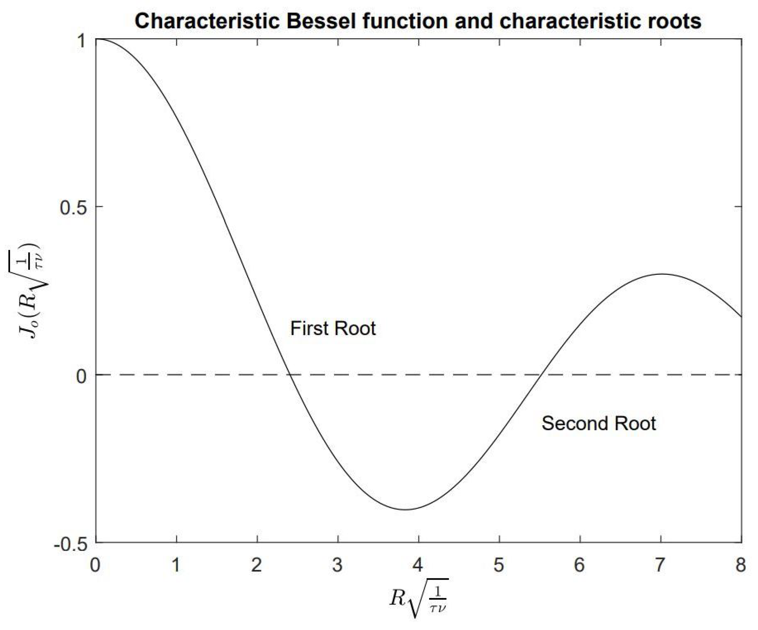
Again, in this paper, for initial validation, water is employed as a reference Newtonian fluid with a dynamic viscosity of , which is equivalent to and the corresponding kinematic viscosity is , which is equivalent to or . Thus, the first root, based on Equation (14) and depicted in Figure 1, is around and the second root is With the realistic dimensions for the actual fluid dispensing system, namely, the pipe diameter and the pipe length , the first two relaxation times and can be evaluated as 1.0806 s and 0.2051 s, respectively. In general, the higher the dynamic viscosity , the lower the flow rate for the same pressure drop. In fact, for viscous incompressible internal fluid, with a time-dependent pressure applied to the inlet surface and a constant pressure, or ambient pressure, applied to the outlet surface, we can easily establish the transient to steady flow characteristics with the concept of the relaxation time [20,21]. Thus, the smaller the kinematic viscosity, the longer the relaxation time. For transient viscous internal fluid, another set of boundary conditions, namely, a constant volume flow rate or average axial flow velocity with a constant pressure at the outlet, might even trigger more studies and discussions of compressible or almost incompressible fluid with pressure pulse and pressure wave propagation within the pipe, the subject of which will be elaborated in a separate paper. Again, our attention in this paper is focused on the relaxation time for Newtonian fluids and non-Newtonian fluids, with respect to a combination of analytical and computational approaches.
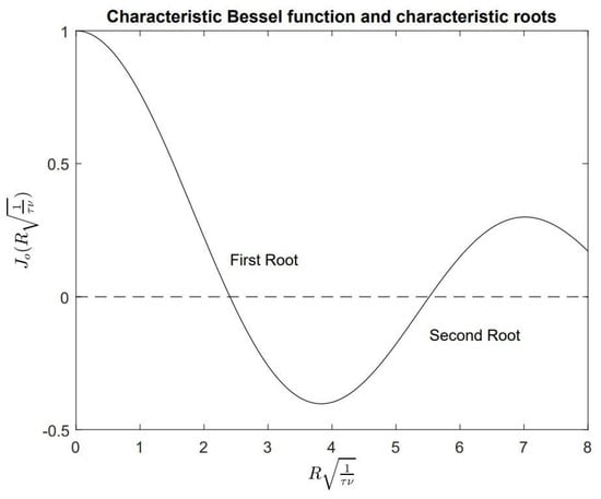
Figure 1.
Eigensolution of the characteristic function and the characteristic time with the root as .
Notice that in comparison with the Newtonian fluid example, in this case, water, the non-Newtonian fluids of interest to us have a similar density, yet the dynamic viscosity is often four million times larger than that of water. Hence, for the same diameter of the pipe, the largest characteristic time or relaxation time could approach a microsecond depending on the flow rate, or rather, the inlet and outlet pressure drop. Nevertheless, in comparison with water, the transient response of these non-Newtonian fluids is much more instantaneous. The relaxation time is visible only when the simulation time step is sufficiently small.
For the pipe’s steady delivery of Newtonian fluid, theoretical solutions as documented in Moody’s chart will be sufficient for the calculation of pressure drop or head loss at different volume flow rate or average axial velocity. Furthermore, we must be aware of the derivation of Equation (1) from the full-fledged Navier-Stokes equations and also identify whether or not the fluid flow is in the turbulent region as well as the transient effects [22,23]. In this study, the precision controls of the intermittent delivery of non-Newtonian fluids depend on a better understanding of the relaxation time, transient behaviors, and the inlet and outlet pressure drops, as well as the volume flow rates with the consideration of nonlinear rheological fluid properties.
3. Computational Approaches
Unlike the purely analytical study of the mixing jet trajectory and the purely computational study of the turbulent mixing jets published earlier by the author [24,25], in this paper, in order to confirm our theoretical predictions with Bessel functions in cylindrical coordinate systems, we have employed the computational fluid dynamics (CFD) feature of the commercial computational mechanics code (ADINA AUI 23 from Bentley Systems) to model the flow within a circular region with various prescribed pressure differentials and ramp sizes [26]. We consider here the transient laminar flow of a homogeneous, viscous, incompressible fluid with constant properties, and obtain the following governing equations from the mass and linear momentum conservation equations:
where , , and stand for fluid mass density, fluid flow velocity in direction , and stress tensor, respectively.
For Newtonian fluids, the stress tensor can be expressed as , where stands for the dynamic viscosity, in fluid mechanics, the respective kinematic viscosity is also defined as , and the shear stress tensor can be denoted as
For non-Newtonian fluids, in this paper, for the shear-thinning fluids of interest to us, we employ a power law model in which the equivalent dynamic viscosity can be expressed as
where A and a, in some literatures, also expressed as , are constants and is the effective deformation rate or shear rate defined as
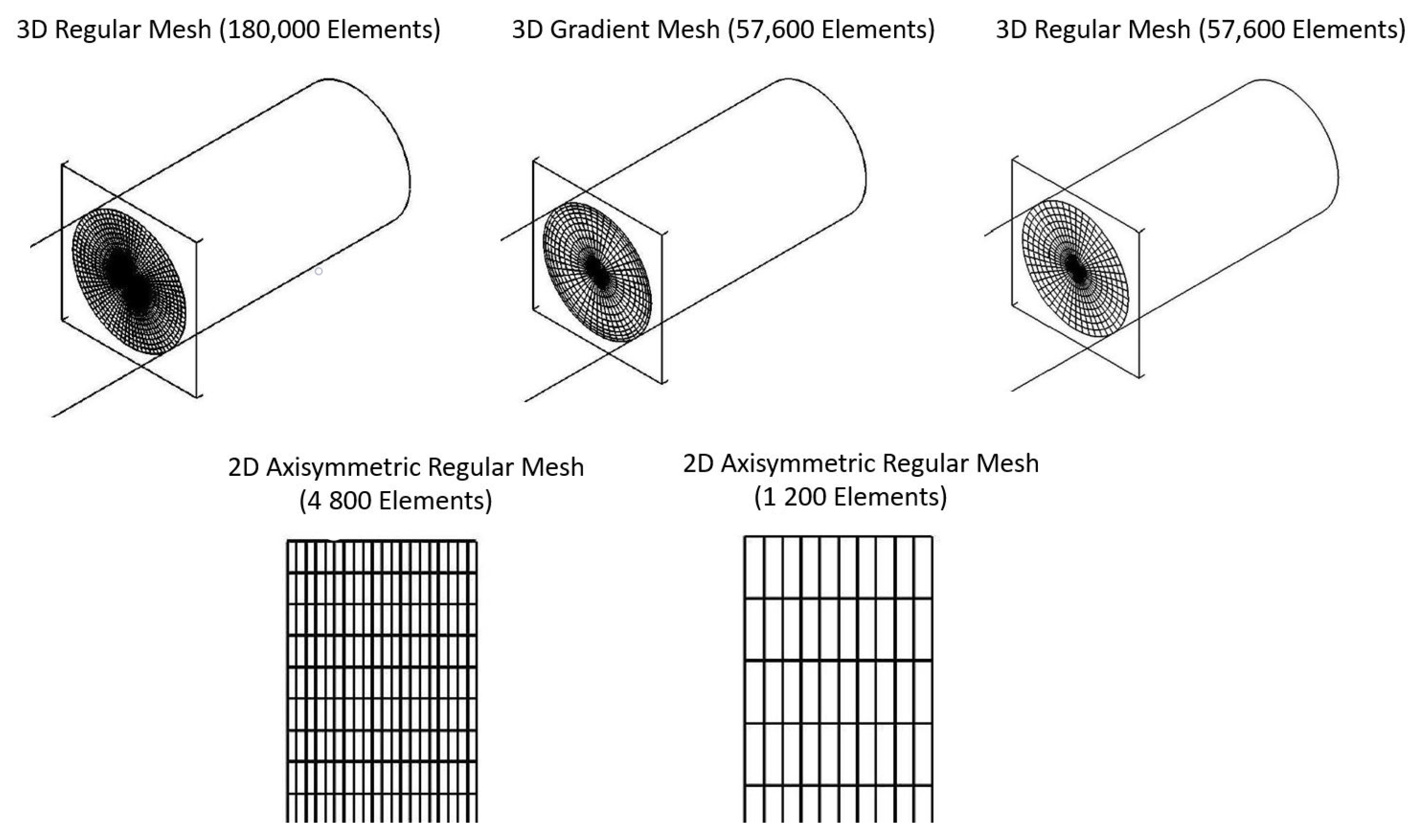
In this study, the polymers of interest have a clear display of shear thinning effects, namely, or , as documented in Refs. [27,28]. The governing equations in Equation (17) are implemented in the ADINA-F, Star-CCM, Solidworks Flow Simulations, and ANSYS Fluent programs. In this paper, ADINA AUI 23 from Bentley Systems is employed for both three-dimensional and two-dimensional axisymmetric models which are computed with dimensions close to the actual fluid dispenser utilized in EV manufacturing plants; for instance, the length 0.1 m and the diameter 5 mm. As illustrated in Figure 2, the full-fledged 3D CFD model has 181,351 nodes and 180,000 elements, while the 3D CFD coarse meshes with and without a mesh gradient have 58,201 nodes and 57,600 elements, respectively. The gradient mesh has a length ratio of 0.2. Moreover, the coarse 2D axisymmetric CFD model has 1331 nodes and 1200 elements, whereas the dense 2D axisymmetric CFD model has 5061 nodes and 4800 elements. In this study, all CFD simulations have been carried out on a desktop with an Intel(R) Xeon(R) E-2124G 64-bit CPU at 3.4 GHz with 32 GB RAM (Intel, Santa Clara, CA, USA). For the reference Newtonian fluid, namely, water, the fluid kinematic viscosity is , and the fluid density is . The total cross-sectional area estimate utilized in the three-dimensional CFD model is in comparison with the analytical solution of the pipe cross-sectional area A, namely, , or . It is clear that the computational domain, discretized with finite elements, is fairly close to the mathematical domain. Furthermore, the average axial velocity is calculated as with the pressure differential as .
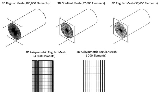
Figure 2.
Different three-dimensional and two-dimensional axisymmetric computational fluid dynamic (CFD) models with a time-dependent pressure inlet and a constant pressure outlet.
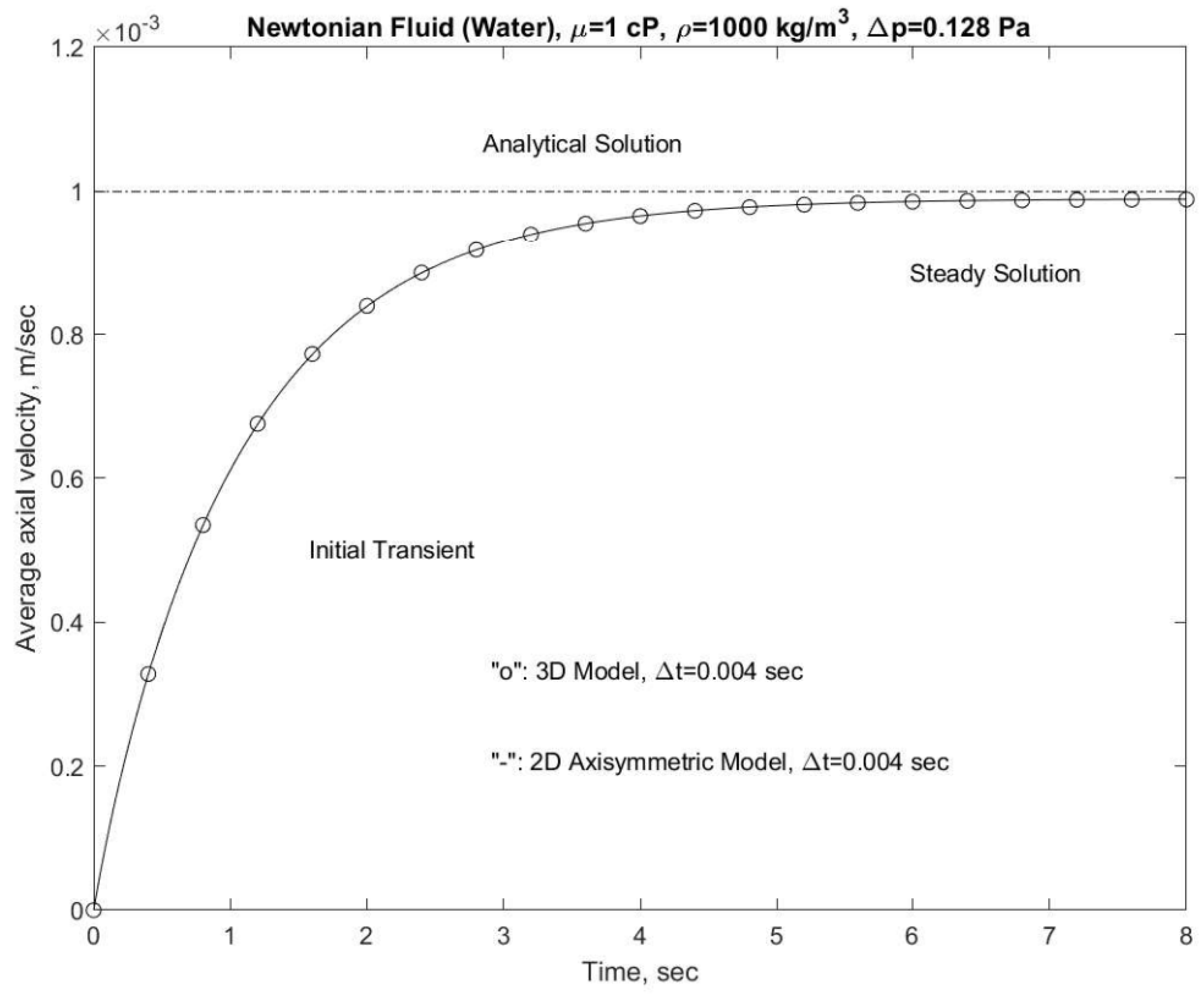
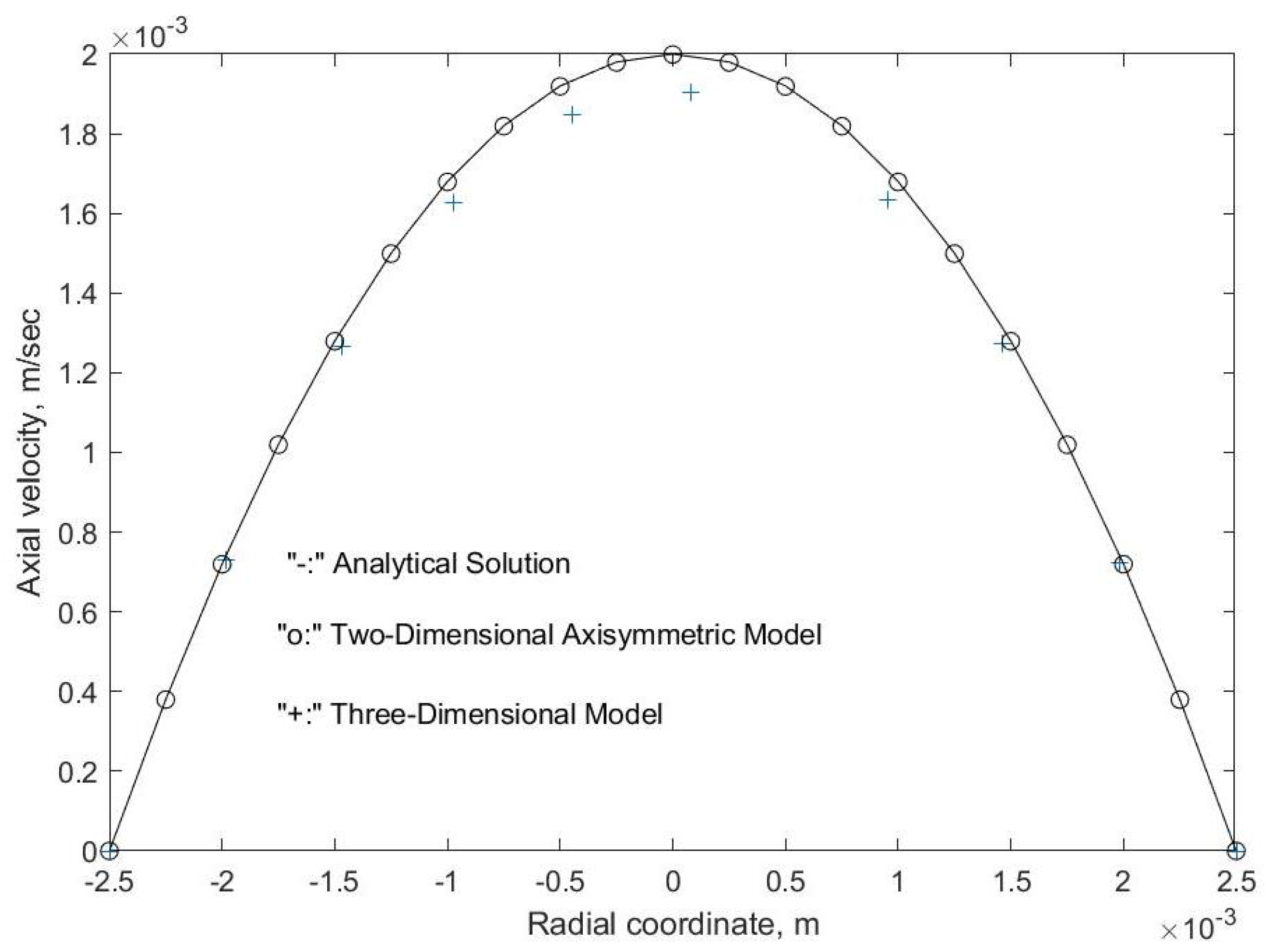
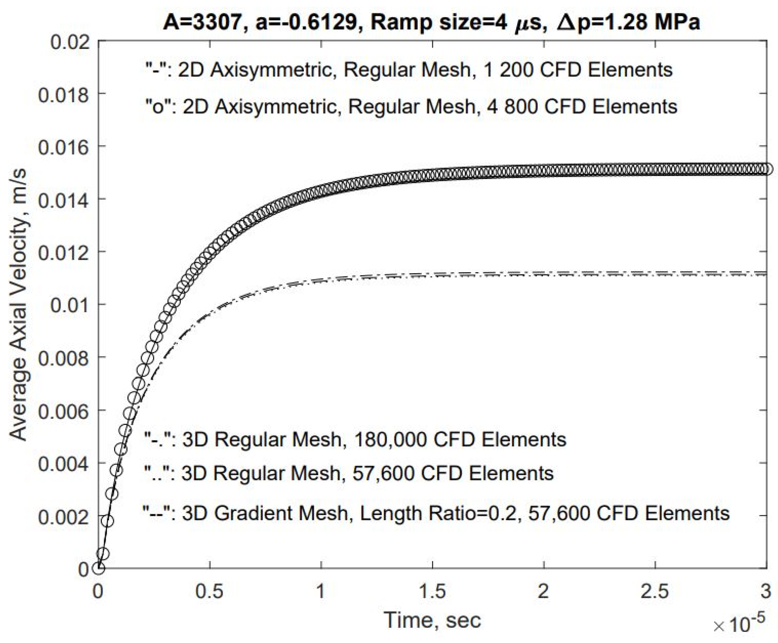
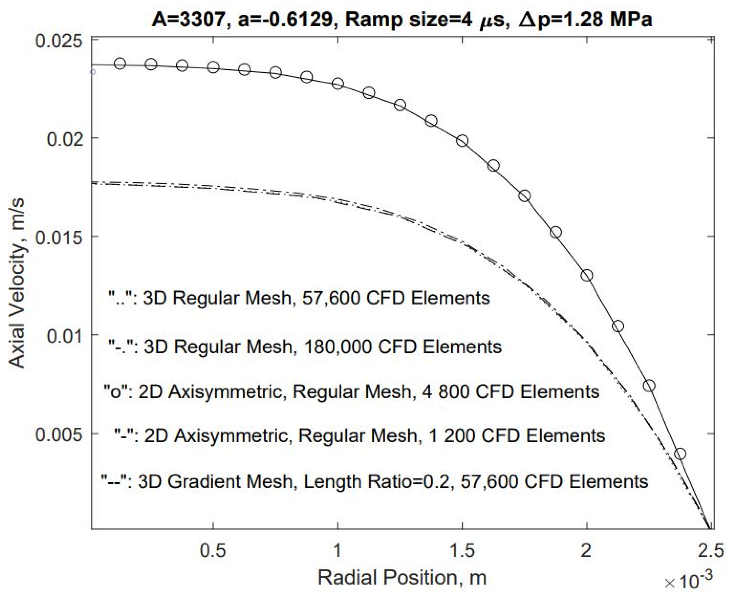
As shown in Figure 3 and Figure 4, the relaxation time predicted in Equation (14) and Figure 1 matches with both 3D and 2D computation models. Furthermore, the fully developed cross-sectional velocity profiles evaluated at a cut surface with a distance of 0.01 m from the outlet for both 3D and 2D models match very well with the analytical solution as stipulated in Equation (5) and shown in Figure 5. In Figure 3 and Figure 4, the transient solutions do approach exponentially to the theoretical or analytical solutions after five or six times the relaxation time. Of course, it is also clear that on a much larger time scale, significantly larger than that of the relaxation time, the computational results will coincide with the theoretical or analytical solutions. It is interesting to note that, as shown in Figure 5, the 2D axisymmetric model does provide better results than the 3D model relative to the analytical approach due to the spatial resolution issues. As shown in Figure 5, it is possible to use a denser mesh in the 2D axisymmetric model, whereas in the 3D model, with a comparable computation cost, a coarser mesh is adopted. It is then clear that in the 2D axisymmetric models, we can afford to use denser meshes for improved spatial resolutions. This, in fact, demonstrates that there is an advantage in implementing 2D axisymmetric models in comparison with comparable 3D models. Similarly, for non-Newtonian fluids, modeled in this study with the power law with , , and , as depicted in Figure 6 and Figure 7, all three 3D models and two 2D models yield comparable results with the identical time function (the ramp size , the time step , and the number of steps 4000). Notice here for non-Newtonian fluids, much smaller time step is adopted in comparison with Newtonian fluids.
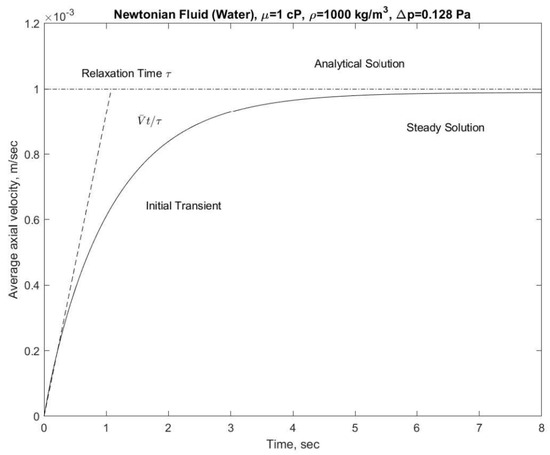
Figure 3.
Relaxation time and initial transient for Newtonian fluid with an inlet pressure impulse and a ramp size 8 ms with a time step 4 ms.

Figure 4.
3D and 2D axisymmetric comparisons of initial transient flow response for Newtonian fluid with an inlet pressure impulse and a ramp size 8 ms with a time step 4 ms.
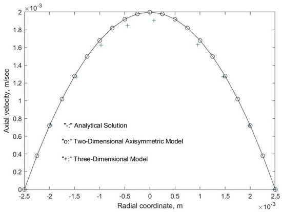
Figure 5.
Computational results in comparison with analytical results for the cross-sectional velocity profile at the fully developed stage, namely, after five or six times the largest or the first relaxation time 1.0806 s.
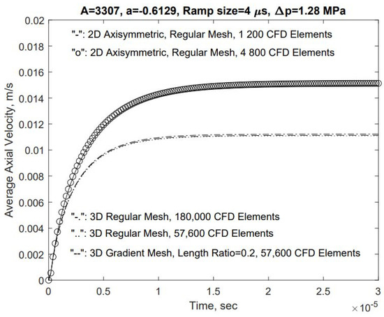
Figure 6.
Time dependent average axial flow velocities in comparison with different 3D and 2D axisymmetric meshes with a ramp size and 4000 time steps with a time step .
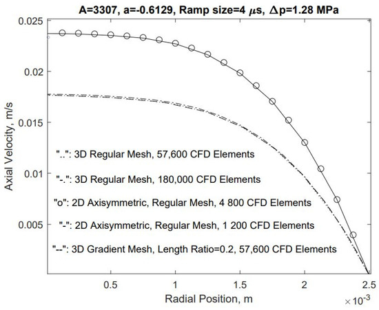
Figure 7.
Cross-sectional velocity profiles at time 0.1 s in comparison with different 3D and 2D axisymmetric meshes.
In fact, as illustrated in Figure 7, unlike the parabolic distribution, the fully developed cross-sectional velocity profile for non-Newtonian fluids does resemble the velocity distribution for turbulent flows [29,30]. Furthermore, due to the definition of the effective shear flow rate in non-Newtonian fluid [31,32], although all three 3D CFD models yield almost identical results as well as all two 2D axisymmetric CFD models, there exists a seemingly systematic deference among 3D and 2D models, which might be attributed to the definition of the effective shear rate for 3D and 2D models. Nevertheless, for the non-Newtonian fluid with 4000 steps and a time step , with the full-fledged 3D CFD mesh, the computation time is 320,964.95 s, with the coarse 3D CFD mesh with a gradient, in this case, a length ratio , the computation time is 47,491.26 s, and with the coarse 3D CFD mesh without a gradient, the computation time is 47,504.77 s. These computational costs are virtually prohibitive for parametric studies and engineering designs. In contrast to these 3D CFD models, for non-Newtonian fluid with 4000 steps and a time step of , with the coarse 2D axisymmetric model without a gradient, the computation time is 239.72 s, and with the dense 2D axisymmetric model without a gradient, the computation time is 1068.76 s. It is therefore clear that we must use 2D axisymmetric CFD models for physical insights into various design and rheological model variations. The discrepancies between the 2D axisymmetric models and the 3D models shown in Figure 6 and Figure 7 are in fact similar to those of Figure 5. They also suggest that in the 2D axisymmetric models, we can afford to use denser meshes for improved spatial resolutions, which again demonstrates the advantage of employing 2D axisymmetric models in comparison with comparable 3D models.
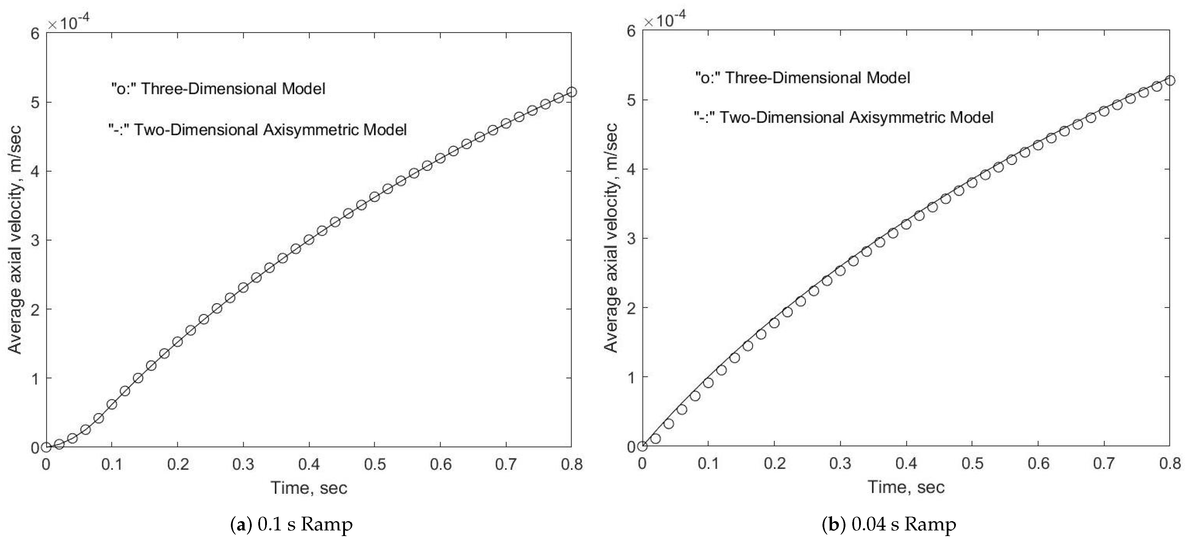
In addition, according to Figure 8, the time-dependent average axial velocity in the transient phase does not depend too much on the size of the time function ramp, which is a piece of important information for the set of boundary conditions with the inlet pressure pulse and the constant outlet pressure. Likewise, the relaxation time is also not altered with the selection of different time step ramps. More importantly, with the same time function with a ramp size of 0.04 s, a time step of 0.02 s, and a number of time steps 40, the computational time for the two-dimensional axisymmetric CFD model is mere 8.25 s with a model with 400 fluid elements and 4411 nodes. Finally, we must note that at the end of 40 time steps, namely, , the total transient solution is still not fully developed since the first or largest relaxation time is as depicted in Figure 4 and Figure 5, therefore the transient responses in Figure 8 suggest that the average axial velocity or the volume flow rate has not reached the fully developed stage. Moreover, as shown in Figure 5, the cross-sectional velocity profiles for the fully developed stage are very close between the analytical solutions in Equation (5) and results from both 3D and 2D axisymmetric models. Note that, just as predicted in Equation (5), the peak velocity in the center of the pipe is two times the average value, which can be easily validated with Equation (7).
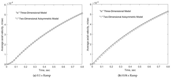
Figure 8.
Averaged velocity as a function of time with large (0.1 s) and small (0.04 s) ramps.
Furthermore, as suggested by Figure 3, Figure 4 and Figure 5, the transient behavior is very much dependent on the relaxation time, as discussed in the analytical part of this study. In fact, based on Equation (13), for Newtonian fluids, the relaxation time depends solely on the pipe radius R and the constant kinematic viscosity . For Newtonian fluids, the higher the radius, the higher the relaxation time; whereas the lower the kinematic viscosity, the higher the relaxation time. In the convergence study with both 3D and 2D CFD models, the computational solution is very close to the analytical prediction based on Moody’s chart or diagram stipulated in Equation (6). More importantly, as predicted by the Bessel function of the first kind, the relaxation time does provide us with an accurate estimate with respect to how long the flow takes to reach the steady solution. With the current configurations, as predicted in Equation (14) and depicted in Figure 1, the dominant, or rather the first relaxation time is 1.0806 s, which matches very well with the computational results in Figure 3 and Figure 4. Moreover, around the origin, the exponential curve for the dominant relaxation expressed as in Equation (15) can be simplified as as illustrated by the tangent in Figure 3. This information is important in the design of a dispensing system. Moreover, for the axisymmetric two-dimensional model, FCBI-C elements, as elaborated in Ref. [33], are introduced, which carry less numerical dissipation. Moreover, we also discover that the regular finite element does provide better accuracy than unstructured mesh.
We did model all non-Newtonian fluid models with three different 3D CFD models as well as comparable 2D axisymmetric computational models. Figure 6 clearly suggests that the relaxation times for non-Newtonian fluids are extremely small in comparison with those for Newtonian fluids. In fact, the initial transient of the volume flow rate or average axial velocity follows closely with the transient inlet pressure pulse defined by the ramp size. Notice, however, for non-Newtonian fluids, that the effective kinematic viscosity will be different for different pressure differentials or volume flow rates. Therefore, an in-depth study of the non-Newtonian fluid behaviors, especially with intermittent precision controls for different types of glues introduced in EV manufacturing plants, is essential and very much needed.
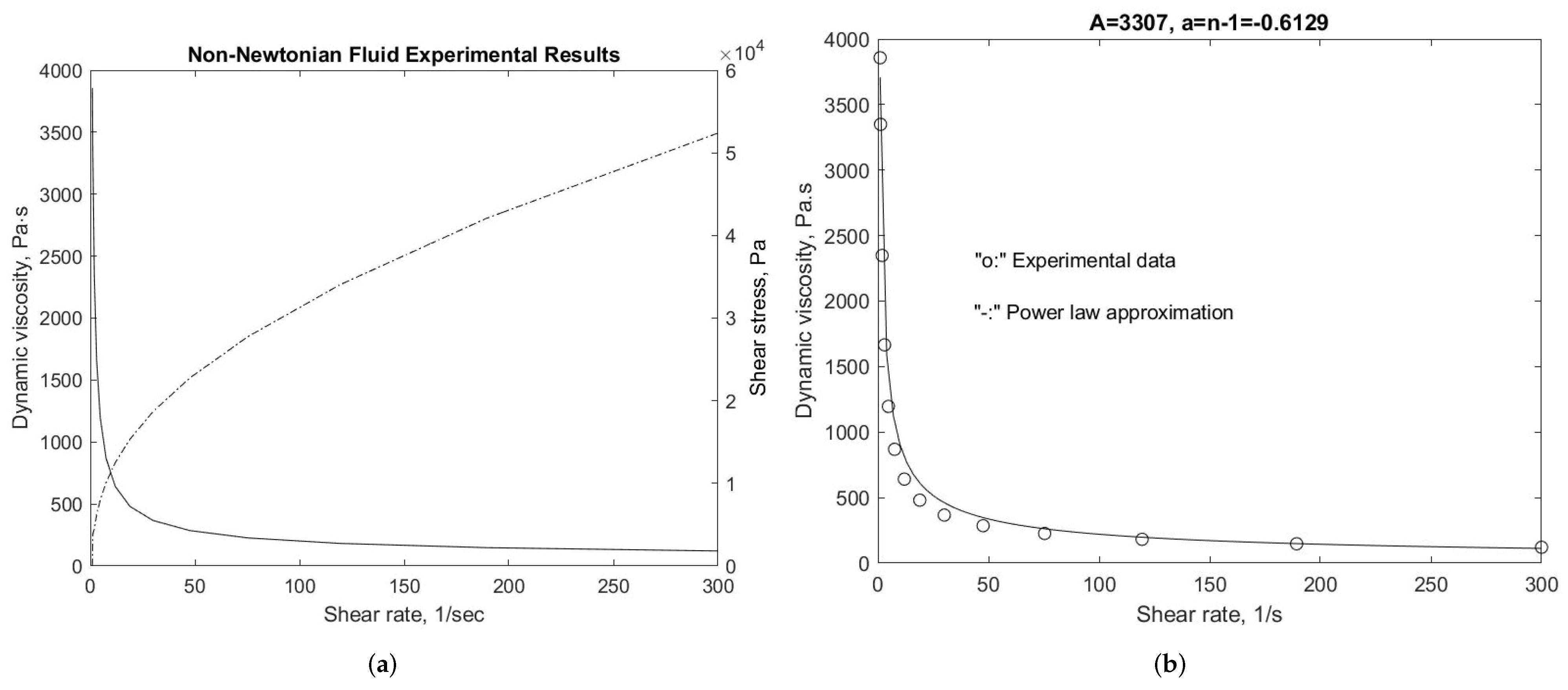
In engineering design, sometimes it is more direct to relate the shear stress with the shear rate . There are in general two types of non-Newtonian fluids, namely, shear thinning and shear thickening. In this paper, we adopt the rheological properties of the non-Newtonian fluid as depicted in Figure 9, which is clearly a shear-thinning fluid [27,34]. We did condense the dynamic viscosity and shear stress as functions of shear rate in Figure 9. These characteristic curves for non-Newtonian fluids represented by a power law are directly derived based on the results of experiments using those glues for EV manufacturing. Such a rheological property is based on the direct experimental measurements of various polymers utilized in car industries. Moreover, from the force equilibrium between the shear force F and the pressure drop , it is obvious that the high pressure drop produces high shear stress.

Figure 9.
Non-Newtonian polymer rheological properties and power law approximations. (a) Rheology; (b) Power Law.
In the ADINA CFD simulation, with , the build-in power law distribution is expressed as
where is the shear rate and stands for the shear stress.
Assume that we have a set of I experimental observations with to I. We would like to find out the best choices for these two parameters, A and a. Let’s say we would like to employ as a curve fitting the experimental data. If such a curve fits perfectly, we then have an equation for each measurement with to I. In reality, there will always be an error in each observation with . Overall, to have the so-called best fit, we need to minimize the total error
Notice here that we use the square of the difference between and just to make sure that the errors will not cancel each other out. Based on the optimization concept discussed in Ref. [4], we discover immediately that the gradient or derivative with respect to and a must be zero, which yields the following equation, the so-called normal equation,
where the unknown vector is with and
Equation (22) is indeed the projection of the original curve-fitting equation
which requires the observation data represented by the vector within the subspace spanned by the columns of the coefficient matrix .
Based on the tabulated relationship between the dynamic viscosity and the shear rate obtained through a series of experiments, utilizing the definition of the dynamic viscosity for a Newtonian fluid,
we have the expression for the shear stress for the non-Newtonian fluid,
With the initial condition with , we can easily derive the relationship between the shear stress and the shear rate based on the relationship between the dynamic viscosity and the shear rate , with ,
For this shear-thinning polymer melt, we can easily draw the conclusion that the effective viscosity for high pressure drop or high shear stress is smaller; thus, the average axial velocity will be larger and the relaxation time will be larger as well. With this prescribed linear regression and normal equation, it is not difficult to come up with the constant A and the power a, in this case, and respectively. Note that the non-Newtonian fluid with or is also called pseudo-plastic. Of course, regression analysis can be used to come up with other non-Newtonian rheological properties, such as the Carreau model in Ref. [35]. As shown in Figure 9, these parameters yield a very close relationship between the dynamic viscosity and the shear rate .
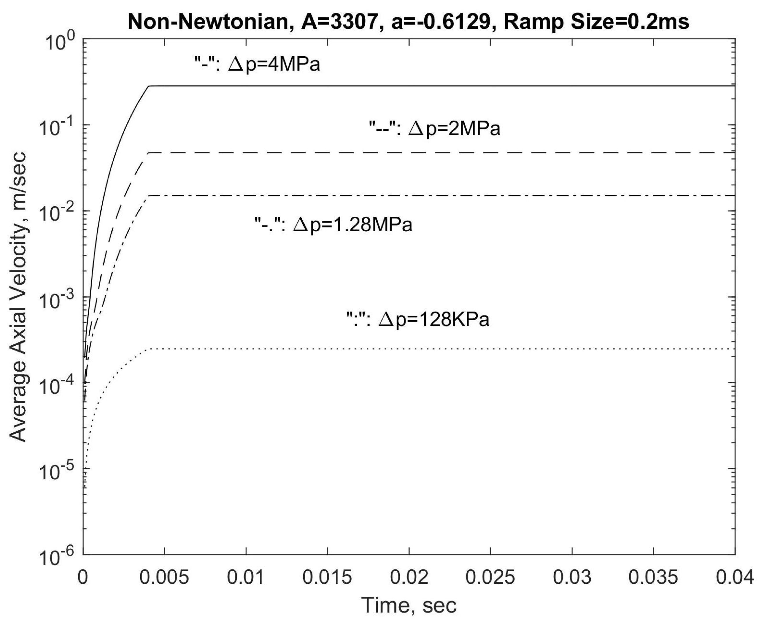
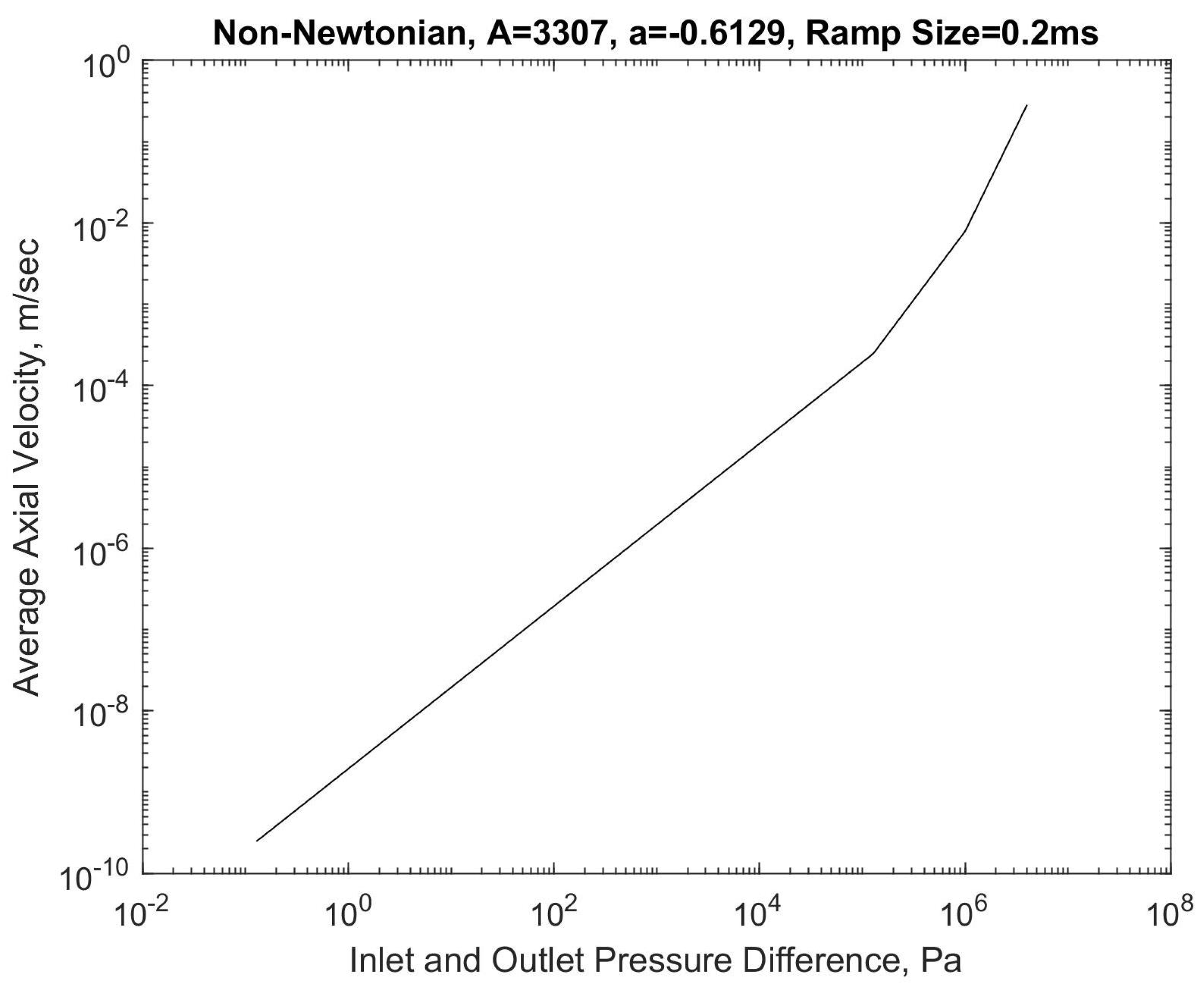
In order to identify the corresponding relaxation time for the non-Newtonian polymer melt, which cannot be easily derived with analytical studies, a series of CFD models have been employed, as depicted in Figure 10 and Figure 11, with a sufficiently small time step of and a ramp size of , respectively. In Figure 10 and Figure 11, semi-logarithmic and logarithmic scales are introduced to depict the average axial velocity results for different pressure drops ranging from to 4 MPa. Furthermore, as long as the shear rate is sufficiently small, namely, the pressure drop is sufficiently small, a constant minimum dynamic viscosity will be introduced instead of the power law distribution, which explains the sudden transition in Figure 10 and Figure 11. In fact, with such a time step, with compressible or nearly compressible fluid models, pressure wave propagations will also be captured. In this paper, we focus on the initial transient effects and the steady solutions. The pressure waves and respective fluid-structure interaction (FSI) physical phenomena will be addressed in a separate paper.
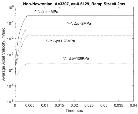
Figure 10.
Average axial velocity transient for the non-Newtonian fluid with the time step 0.1 ms and the ramp size 0.2 ms.

Figure 11.
Average axial velocity and the inlet and outlet pressure drop relationship for the non-Newtonian fluid with the time step 0.1 ms and the ramp size 0.2 ms.
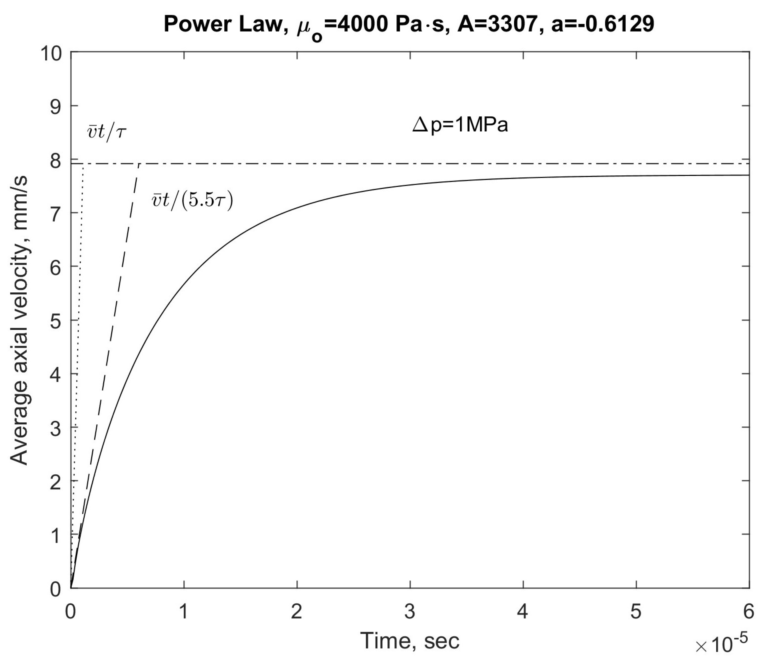
It is clear based on the CFD results depicted in Figure 12, Figure 13, Figure 14 and Figure 15, with the small ramp size and the corresponding time step, relaxation times do exist in initial transients along with the steady solution. Moreover, since the 2D axisymmetric cases are comparable with the respective three-dimensional cases and the computation times are much smaller, a sufficiently large number of time steps and cases with various inlet and outlet pressure drops have been computed for further validations. For the inlet and outlet pressure drop 1 MPa, based on Equations (6) and (8), we can establish the effective dynamic viscosity for this non-Newtonian polymer melt as
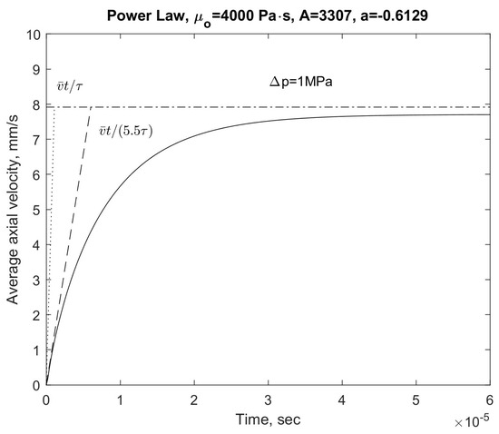
Figure 12.
Average axial velocity profile with the consideration of relaxation time for the non-Newtonian fluid with the pressure drop 1 MPa, the time step 0.2 , and the ramp size 0.4 .
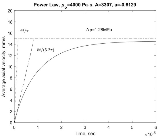
Figure 13.
Average axial velocity profile with the consideration of relaxation time for the non-Newtonian fluid with the pressure drop 1.28 MPa, the time step 0.2 , and the ramp size 0.4 .
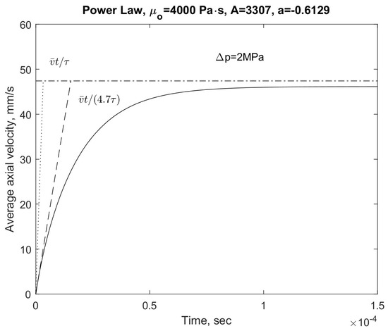
Figure 14.
Average axial velocity profile with the consideration of relaxation time for the non-Newtonian fluid with the pressure drop 2 MPa, the time step 0.2 , and the ramp size 0.4 .
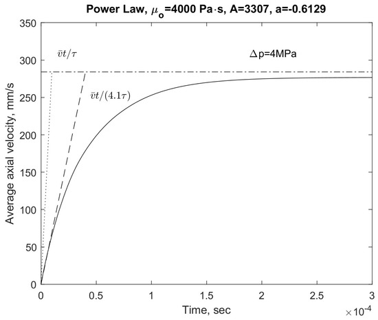
Figure 15.
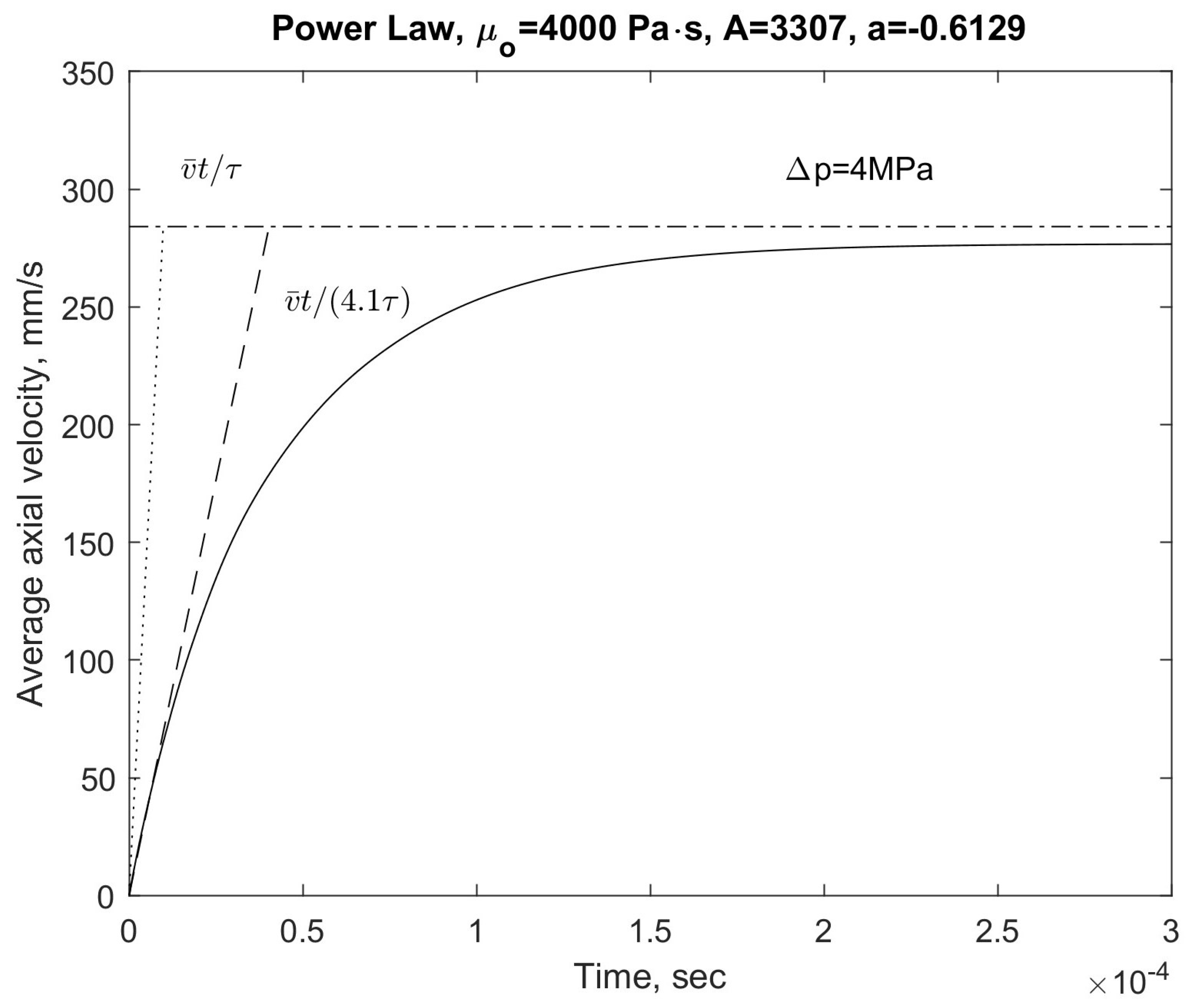
Average axial velocity profile with the consideration of relaxation time for the non-Newtonian fluid with the pressure drop 4 MPa, the time step 0.2 , and the ramp size 0.4 .
Notice that for a Newtonian fluid, as long as the fluid is laminar, the average velocity will be proportional to the pressure drop, which might be extended to non-Newtonian fluid at that particular inlet and outlet pressure drop. Consequently, assuming the approximate density of the polymer melt is similar to that of water, namely, , we have the corresponding effective kinematic viscosity
Furthermore, according to the discussion of the relaxation time for a Newtonian fluid based on the zeroth order Bessel function of the first kind in Equation (14), the effective relaxation time is evaluated as
where the radius of the pipe R is 2.5 mm and the first root of the zeroth order Bessel function of the first kind equals .
As illustrated in Figure 12, Figure 13, Figure 14 and Figure 15, similar relaxation times exist for non-Newtonian fluids just as those for Newtonian fluids as depicted in Figure 3, Figure 4 and Figure 8. However, for non-Newtonian fluids, the nonlinear dynamic viscosity depends on the shear rate or the axial fluid flow velocity, which is a function of the inlet and outlet pressure drop or difference. Thus, a so-called multiplier can be introduced to adjust the relaxation time derived from the relationship as presented in Equation (14) and depicted in Figure 1. In fact, as illustrated in Figure 12, the equivalent relaxation time seems to be closer to the overall viscous effect of the non-Newtonian fluid. Therefore, we introduce in this paper a so-called 2D axisymmetric multiplier . This suggests that, with respect to the calculation of the relaxation time, the dynamic viscosity is actually times smaller than the effective dynamic viscosity. With this comprehensive understanding of the effects of the ramp size with respect to the relaxation time and the final steady solution, which is independent of the ramp size, we can now proceed to change the peak pressure drop and establish its nonlinear relationship with the steady solution represented by the average pipe velocity [18,36]. The steady state volume flow rate, average axial velocity, effective dynamic viscosity, relaxation time, and 2D axisymmetric multiplier corresponding to the peak inlet and outlet pressure drop at 1, , 2, and 4 MPa are tabulated in Table 1. In comparison with the case of the Newtonian fluid, the transient behaviors of the non-Newtonian fluid are definitely much more complex [27,34]. The computational results do demonstrate that due to the shear rate-induced thinning, namely, the effective dynamic viscosity decreases with the increase of the shear rate and the effective relaxation time will increase, which corresponds to the decrease of the slope of the initial tangent. It is interesting to point out that the 2D axisymmetric multiplier does experience a slight and insignificant decrease. Moreover, a power law similar to that for the non-Newtonian rheology is introduced to link these key results with the peak pressure drop. These power laws will provide designers and operators with much-needed guidelines in the precision controls of intermittent delivery of these non-Newtonian fluids.

Table 1.
Volume flow rate, average axial velocity, effective dynamics viscosity, effective relaxation time, and 2D axisymmetric multiplier with respect to the pressure difference.
With merely two times the peak pressure drop, namely, increases from 2 MPa to 4 MPa, the average velocity for the steady solution is more than quadrupled, namely, increases from 47.4075 mm/s to 284.1155 mm/s; the same for the volume flow rate, namely, increases from to or cc/s. Consequently, the effective dynamic viscosity, namely, , decreases from to , whereas the effective relaxation time, namely, , increases from to These tabulated results match with the displays according to Figure 12, Figure 13, Figure 14 and Figure 15.
In this study, for the specific implementation in the power law of the non-Newtonian fluid, a cut-off dynamic viscosity of is introduced along with the coefficient and the power . As a result, when the inlet and outlet pressure drop is sufficiently low, namely, the shear rate is sufficiently low, instead of having an extremely high value of the effective dynamic viscosity, a cut-off dynamic viscosity is implemented in the CFD model. Thus, the transient behaviors of the non-Newtonian fluid remain the same during the very low shear laminar flow region, similar to the case for a Newtonian fluid.
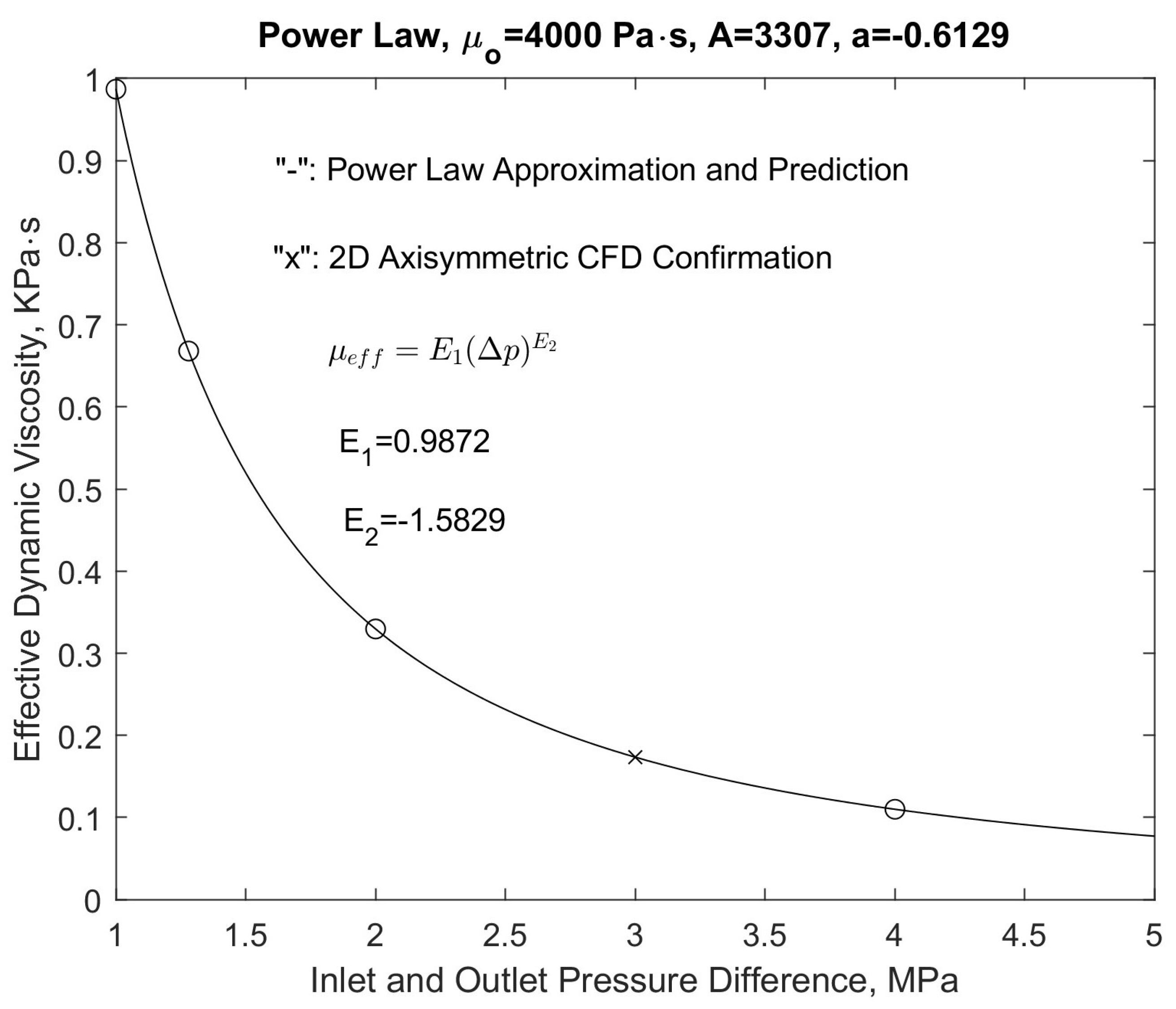
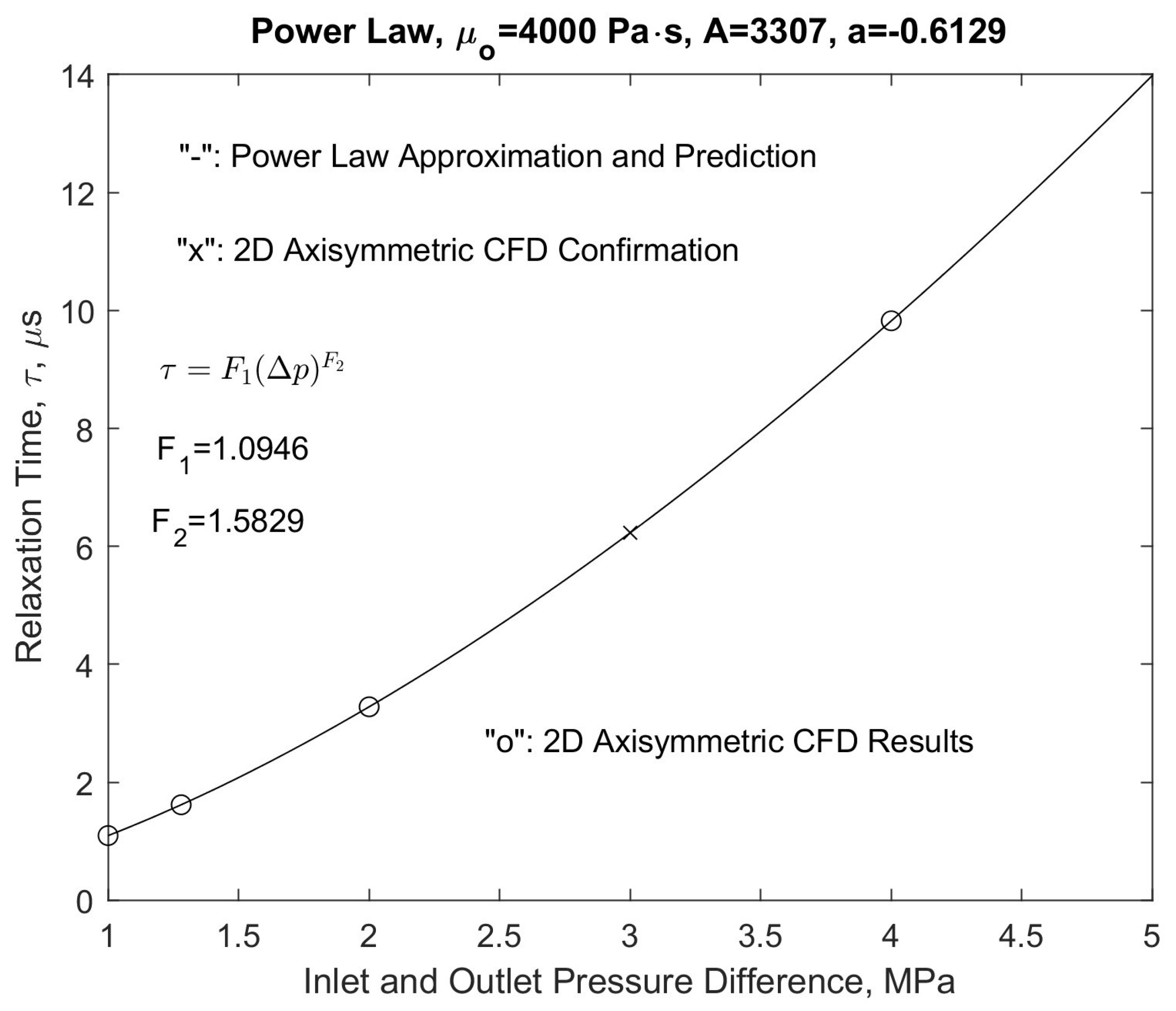
Furthermore, the shear thinning effect represented by a typical power law yields, as shown in Figure 12, Figure 13, Figure 14 and Figure 15, a relationship similar to non-Newtonian rheologies modeled in Figure 9. To reiterate, as we increase the peak pressure from 1 to 4 MPa, the effective dynamic viscosity is significantly reduced, thus the effective kinematic viscosity is significantly decreased, and the relaxation time is increased accordingly. In addition, the 2D axisymmetric multiplier decreases from to Figure 16, Figure 17 and Figure 18 again demonstrate clearly the thinning effect, which is consistent with what the rheological properties suggest for this type of polymer melt. To reiterate, under sufficient pressure drop, the effective kinematic viscosity will decrease significantly, and as a result, the relaxation time will increase accordingly.
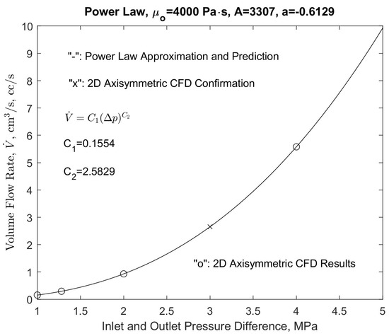
Figure 16.
Pressure drop vs. volume flow rate .
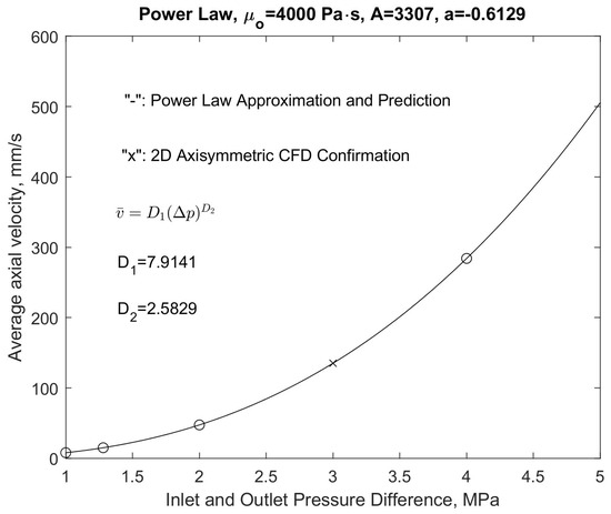
Figure 17.
Pressure drop vs. average axial velocity .

Figure 18.
Pressure drop vs. effective dynamics viscosity .
As shown in Figure 12, Figure 13, Figure 14 and Figure 15, the steady solution yields a significantly larger average velocity, which confirms that the effective viscosity is much smaller. In addition, the multiplier for the relaxation time changes from to , which indicates that the equivalent relaxation time decreases according to the effective kinematic viscosity and, more importantly, gets closer to the relaxation time predicted with the effective kinematic viscosity. Moreover, to depict the thinning effects, we also plot the pressure drop in vs. the steady flow rate defined as in as shown in Figure 16 as well as the pressure drop in vs. the effective relaxation time in as shown in Figure 19.

Figure 19.
Pressure drop vs. effective relaxation time .
Moreover, in order to derive empirical power laws for the relationship between the pressure drop and the volume flow rate , the average axial velocity , the effective dynamic viscosity , the corresponding relaxation time , and the multiplier , the following power laws or the equivalent logarithmic forms are introduced
Using the same projection method for the normal equations as we have employed for the power law rheological relationship between the shear rate and the dynamic viscosity, the coefficient solutions for these power laws can be easily derived, namely, and are and , respectively; and , are and , respectively; and are and , respectively; and are and , respectively; and and , are and , respectively. As a consequence, using the power laws, we can predict a priori the transient flow response for the inlet and the outlet pressure differential 3 MPa, marked by a cross, namely, volume flow rate 2.6532 cc/s; average axial velocity 13.5127 mm/s; effective dynamic viscosity 0.1734 ; effective relaxation time ; and 2D axisymmetric multiplier , respectively, which are virtually identical to the 2D axisymmetric CFD simulation results.
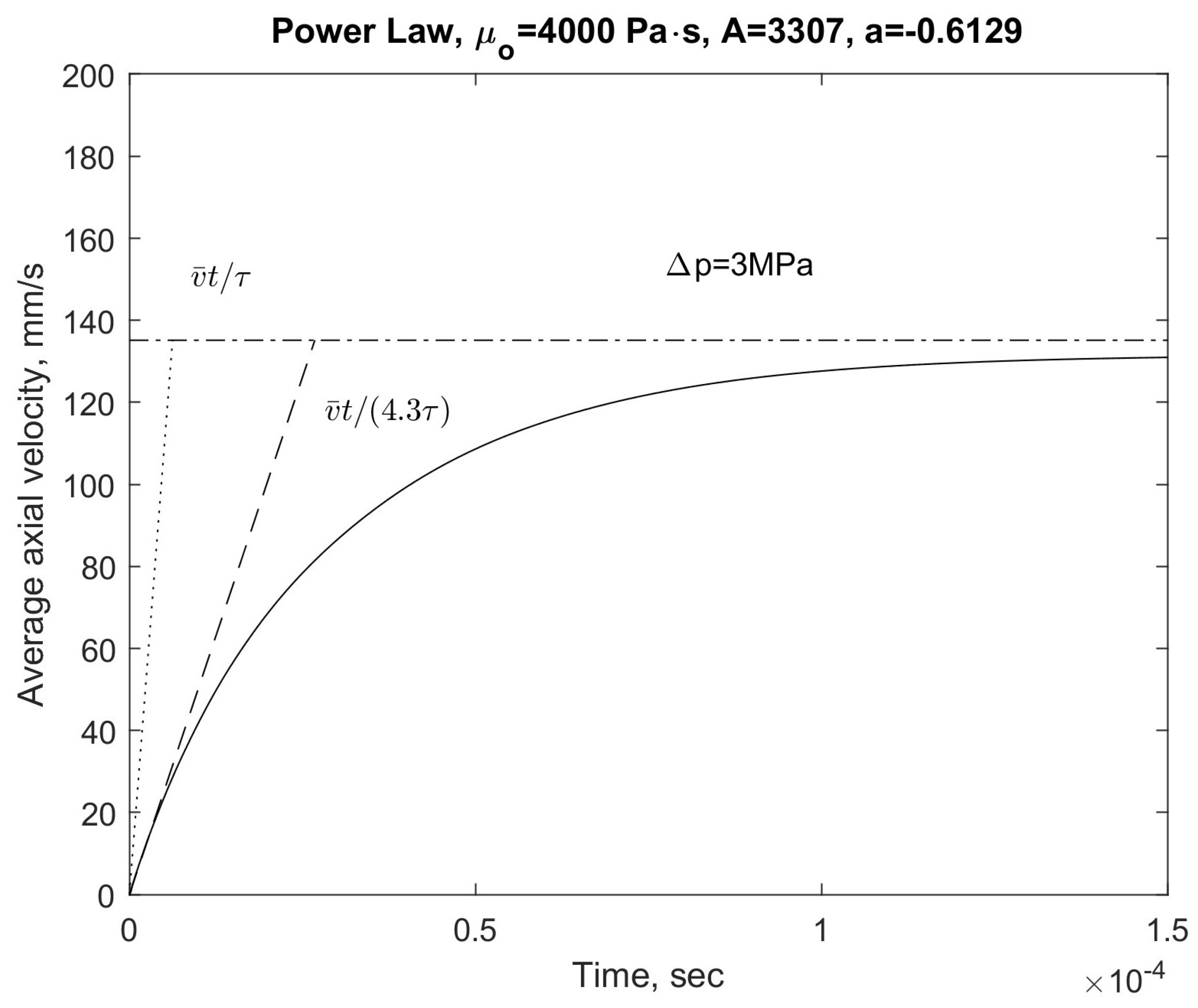
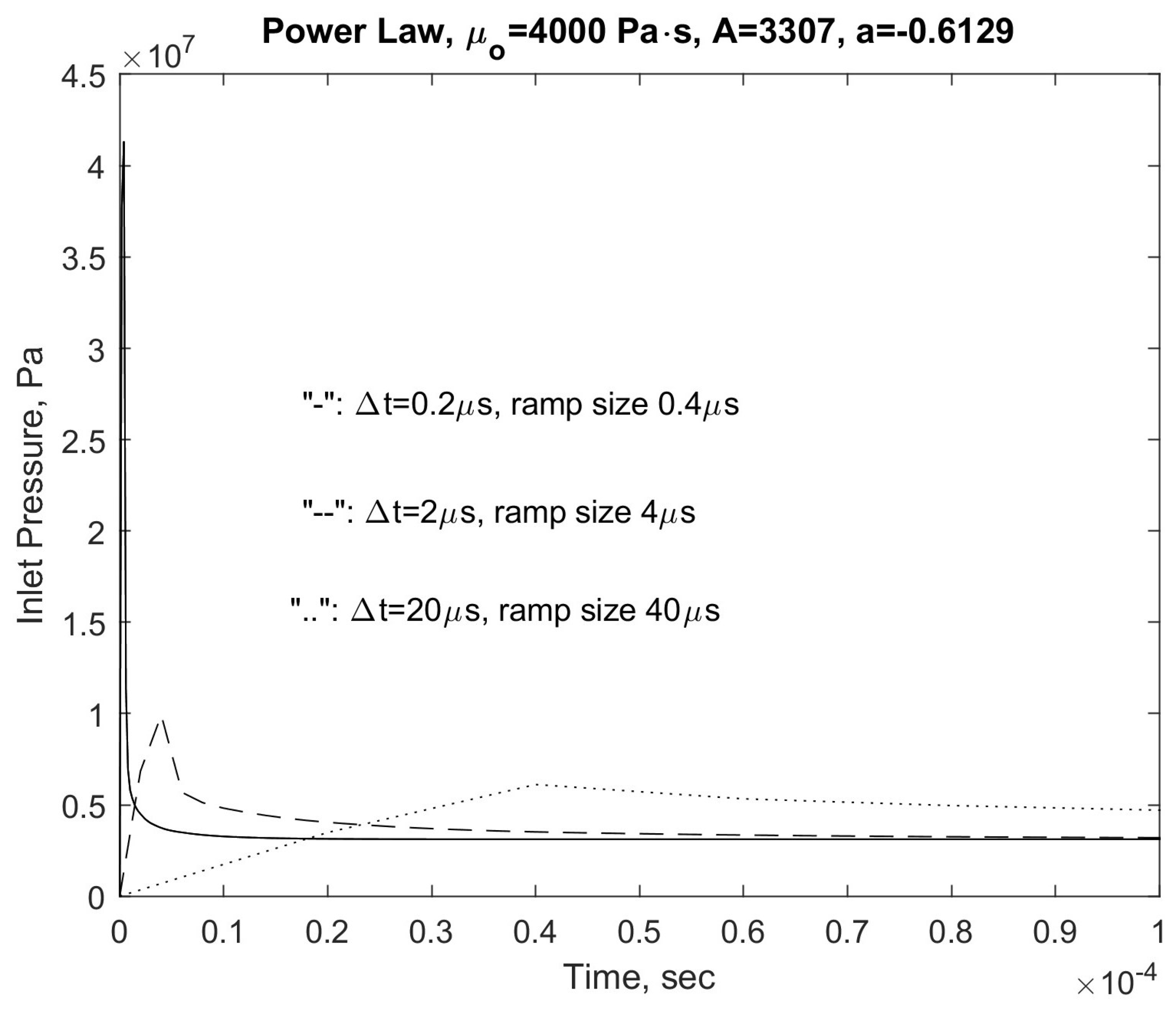
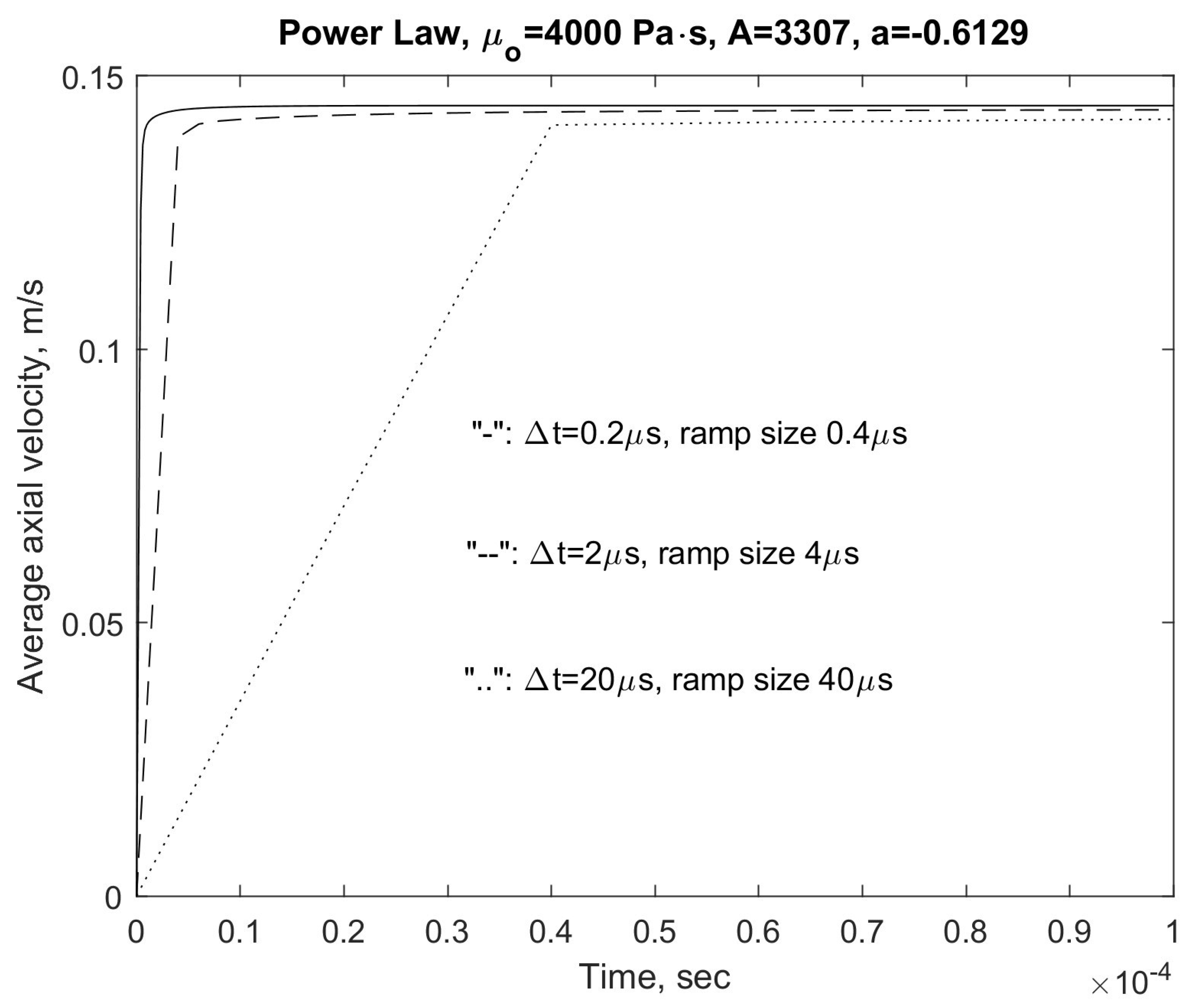
Notice the relationship, especially the power, among the average axial velocity or the volume flow rate , the effective dynamics viscosity , the corresponding relaxation time , and the 2D axisymmetric multiplier . As illustrated in Figure 16, Figure 17, Figure 18, Figure 19 and Figure 20, with the open circle representing the individual cases and the solid line the effective power law relationship, the curve fit is extremely accurate, which suggests that the power law distribution with constant coefficients does match with the physical reality. To test the validity of these approximations, a new peak pressure drop of 3 MPa is selected a priori. With the 2D axisymmetric model, it only takes 177 s per set of test conditions, instead of a few days for the full-fledged 3D model. We have the predicted results using the power law distributions for the volume flow rate, average axial velocity, effective dynamic viscosity, relaxation time, and 2D axisymmetric multiplier match very closely with the computational modeling, namely, 2.6532 cc/s, 135.126 mm/s, , , and , respectively, as denoted with the symbol x in Figure 16, Figure 17, Figure 18, Figure 19 and Figure 20. The fact that the actual simulation results, with a different boundary condition, as reported in Figure 21, match very well with the predictions from the power law distributions a priori confirms the validity of the behaviors of these non-Newtonian fluids modeled with a power law distribution. Finally, to further validate the investigations and conclusions in this paper, we replace the inlet boundary condition with an average axial velocity of 150 mm/s. The steady average inlet pressure as shown in Figure 22 approaches 3 MPa with an average axial velocity around 135 mm/s. As depicted in Figure 22, the inlet pressure does eventually approach the same steady solution regardless of the ramp sizes, in this case, 0.4 s, 4 s, and 40 s, and the time step sizes, in this case, 0.2 s, 2 s, and 20 s. Furthermore, as illustrated in Figure 22 and Figure 23, the choice of the ramp size, which essentially determines how fast the servo motor is actuated, does have tremendous effects on the initial inlet pressure, even for an incompressible non-Newtonian fluid model due to inertia effects. Naturally, to fully understand such phenomena, more complex FSI with the flexible tube and the wave propagations within both fluid and solid continua must be considered. However, it is clear and could be suggested for precision control of the dispensing of non-Newtonian glues in EV manufacturing, the ramp size of the servo motor must be tuned properly to ensure the timely fluid delivery and to suppress unnecessary structure oscillation. As depicted in Figure 22 and Figure 23, the smaller the ramp size, the quicker the servo motor generates the desired volume flow rate and the higher the inlet and outlet pressure drop. We must also point out that the numerical treatment of the average axial velocity has a slight discrepancy in comparison with the volume flow rate due to the actual cross-sectional area representation and the boundary wall conditions. For the 2D axisymmetric CFD mesh, in the cross-sectional direction, 10 CFD elements are employed. In the particular setting of the average axial velocity, the velocity boundary for the wall is zero; thus, the average velocity is in effect applied to nine out of the ten elements, which accounts for the discrepancy of 150 mm/s vs. 135 mm/s average axisymmetric velocity. In most engineering practices, however, such accuracy with a relatively coarse CFD mesh does provide engineers with important guidelines in the selection of operation parameters in the controlled intermittent distributions of such non-Newtonian fluids.
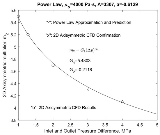
Figure 20.
Pressure drop vs. 2D multiplier .

Figure 21.
Two-dimensional axisymmetric model for peak pressure drop 3 MPa, which matches with the prediction with the power laws.
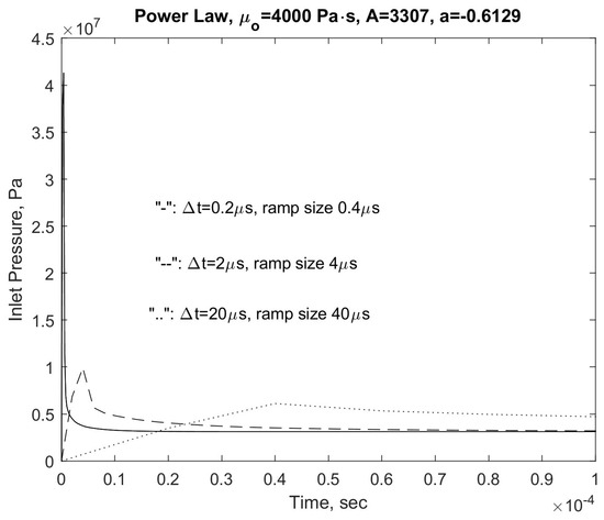
Figure 22.
Inlet pressure time-dependent response for two-dimensional axisymmetric model with an average axial velocity 150 mm/s.
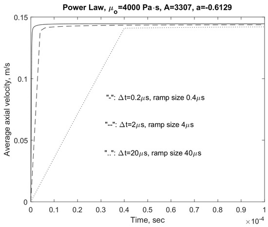
Figure 23.
Axial time-dependent flow for two-dimensional axisymmetric model with an average axial velocity 150 mm/s.
4. Conclusions
In this paper, through a combination of theoretical and computational studies, we demonstrate and reiterate the inner connections between the pressure drop and the volume flow rate for Newtonian and non-Newtonian incompressible fluids. The prediction of pressure loss within fully developed and steady pipe flow systems can be fairly accurately predicted with Moody’s Chart or Diagram along with respective major and minor friction losses. However, in EV manufacturing plants, the precision controls of the intermittent delivery of glues require a good understanding of these complex fluids’ transient or developing behaviors. Moreover, it is also confirmed that relaxation time does exist for both Newtonian and non-Newtonian fluids. In general, the relaxation time is inversely proportional to the effective kinematic viscosity and the square of the pipe radius. In addition, the relaxation time is independent of the ramp size for the inlet pressure impulse. With the confirmation and reiteration of the relaxation time for Newtonian fluid with the linear relationship between the shear stress and the shear rate, the concept of the relaxation time is also expanded to non-Newtonian fluid with respect to the magnitude of the shear stress, which is directly linked to the volume flow rate, hence the pressure drop magnitude, both of which are important design parameters. Furthermore, the relaxation time, volume flow rate, and average axial velocity for non-Newtonian fluids can also be linked to the inlet and outlet pressure drops through a power law relationship.
This paper introduces a shear-thinning non-Newtonian fluid model with a power law relationship between the effective dynamic viscosity and the effective shear rate, along with a cut-off dynamic viscosity . The precise deliveries of non-Newtonian fluids depend on many factors, such as the effective relaxation time, inlet and outlet pressure differential, rheology of non-Newtonian fluids, displacement-controlled or transient force, or pressure-controlled inlet condition. In fact, through experiments in some specific conditions, the pressure wave propagation within the fluid can also be present and pose unique challenges to dispensing systems. We also recognize that the rheological properties may vary with temperature, which must be addressed separately in concert with the detailed designs of dispensing systems.
Finally, the authors must emphasize through this systematic study of the intermittent dispensing of non-Newtonian fluids that the full-fledged three-dimensional CFD models must be applied judiciously because of their cost and massive computation details. Hierarchical studies with more physical insights are always preferred in engineering practice, especially during the initial design phases. Finally, the power law relationships between the steady state inlet and outlet pressure difference and the volume flow rate, average axial velocity, effective dynamic viscosity, relaxation time, and 2D axisymmetric multiplier, respectively derived from a series of systematic transient CFD models, predict accurately or nearly exactly a priori the simulation results with other boundary conditions. These empirical formulas derived from both analytical and computational studies will help to design and program precision controls for the delivery of non-Newtonian glues in EV manufacturing plants.
Author Contributions
Conceptualization, S.W. and D.G.; methodology, S.W.; software, S.W., D.G., A.W. and K.B.; validation, S.W. and D.G.; formal analysis, S.W. and D.G.; investigation, S.W., D.G., A.W., K.B. and K.W.; resources, S.W. and D.G.; data curation, S.W. and D.G.; writing—original draft preparation, S.W. and D.G.; writing—review and editing, S.W., D.G., A.W., K.B. and K.W.; visualization, S.W.; supervision, S.W. and D.G.; project administration, S.W. and D.G.; funding acquisition, S.W. and D.G. All authors have read and agreed to the published version of the manuscript.
Funding
This research was partially supported by GM Research Grant.
Data Availability Statement
The original contributions presented in the study are included in the article, further inquiries can be directed to the corresponding author.
Acknowledgments
We would like to thank Christian Proteau in Famic Technologies Inc. in Montreal Canada, Shanhong Ji in ADINA, Inc., and Brink and Azzouz at MSU Texas for their assistance. We are also grateful to Global Technical Center of General Motors in Warren, MI for their financial supports.
Conflicts of Interest
The authors declare that this study received funding from GM Research Grant. The funder was not involved in the study design, collection, analysis, interpretation of data, the writing of this article or the decision to submit it for publication. Author Dalong Gao was employed by the GM Corporation. The remaining authors declare that the research was conducted in the absence of any commercial or financial relationships that could be construed as a potential conflict of interest.
References
- Bucalem, M.; Bathe, K. The Mechanics of Solids and Structures-Hierarchical Modeling and the Finite Element Solution; Springer: Berlin/Heidelberg, Germany, 2011. [Google Scholar]
- Wang, S.; Ndip-Agbor, E.; Atamenwan, E. On Hierarchical Applications of Finite Element Methods and Classical Applied Mechanics Approaches for Complex Structures. Appl. Mech. 2022, 3, 464–480. [Google Scholar] [CrossRef]
- Wang, S.; Rowlan, L.; Henderson, A.; Aleman, S.T.; Creacy, T.; Taylor, C.A. Viscoelastic Representation of the Operation of Sucker Rod Pumps. Fluids 2022, 7, 70. [Google Scholar] [CrossRef]
- Wang, S. Essential Mathematical Tools for Engineers; Sentia Publishing: Lakeway, TX, USA, 2022. [Google Scholar]
- Wang, S. Scaling, Complexity, and Design Aspects in Computational Fluid Dynamics. Fluids 2021, 6, 362. [Google Scholar] [CrossRef]
- Klein, A. Review: Turbulent Developing Pipe Flow. J. Fluids Eng. 1981, 103, 243–249. [Google Scholar] [CrossRef]
- Al-Nassri, S.; Unny, T. Developing Laminar Flow in the inlet length of a smooth pipe. Appl. Sci. Res. 1981, 36, 313–332. [Google Scholar] [CrossRef]
- Gerhart, P.; Gerhart, A.; Hochstein, J. Fundamentals of Fluid Mechanics; Wiley: Hoboken, NJ, USA, 2016. [Google Scholar]
- Durst, F.; Ray, S.; Unsai, B.; Bayoumi, O. The Development Lengths of Laminar Pipe and Channel Flows. J. Fluids Eng. 2005, 127, 1154–1160. [Google Scholar] [CrossRef]
- Sparrow, E.; Lin, S. The Developing Laminar Flow and Pressure Drop in the Entrance Region of Annular Ducts. J. Fluids Eng. 1964, 86, 827–833. [Google Scholar] [CrossRef]
- Wang, S.; Rowlan, L.; Elsharafi, M.; Ermila, M.; Grejtak, T.; Taylor, C. On Leakage Issues of Sucker Rod Pumping Systems. ASME J. Fluids Eng. 2019, 141, 111201–111207. [Google Scholar] [CrossRef]
- White, F. Viscous Fluid Flow; MacGraw-Hill: New York, NY, USA, 1991. [Google Scholar]
- Khamoushi, A.; Keramat, A.; Majd, A. One-Dimensional Simulation of Transient Flows in Non-Newtonian Fluids. J. Pipeline Syst. Eng. Pract. 2020, 11, 04020019. [Google Scholar] [CrossRef]
- Khamoushi, A.; Keramat, A.; Majd, A. One-Dimensional Simulation of the Water Hammer Phenomenon in Non-Newtonian Fluids. J. Civ. Eng. 2020, 52, 225–242. [Google Scholar]
- Achard, L.; Lespinard, G. Structure of the transient wall-law in one-dimensional models of laminar pipe flows. J. Fluid Mech. 1981, 113, 283–298. [Google Scholar] [CrossRef]
- Hristov, J. A Transient Flow of a Non-Newtonian Fluid Modelled by a Mixed Time-Space Derivative: An Improved Integral-Balance Approach. Math. Methods Eng. 2018, 24, 153–174. [Google Scholar]
- Wang, S.; Feng, Z. A Note on Helmholtz Attenuators with Air Cavity and Membrane. In ASME IMECE Proceedings of Dynamic Systems and Control Division; NVC-12; American Society of Mechanical Engineers: Anaheim, CA, USA, 1998. [Google Scholar]
- Bathe, K.; Nitikitpaiboon, C.; Wang, S. A Mixed Displacement-Based Finite Element Formulation for Acoustic Fluid-Structure Interaction. Comput. Struct. 1995, 56, 225–237. [Google Scholar] [CrossRef]
- Wang, S. Fundamentals of Fluid-Solid Interactions-Analytical and Computational Approaches; Elsevier Science: Amsterdam, The Netherlands, 2008. [Google Scholar]
- Back, L.; Crawford, D. Wall shear stress estimates in coronary artery constrictions. J. Biomed. Eng. 1992, 114, 515–520. [Google Scholar] [CrossRef] [PubMed]
- Midvidy, W.; Rouleau, W.T. Stability of Poiseuille Flow in Elastic Tubes. J. Appl. Mech. 1977, 44, 18–24. [Google Scholar] [CrossRef]
- Nouri, J.; Whitelaw, J. Flow of Newtonian and Non-Newtonian Fluids in a Concentric Annulus With Rotation of the Inner Cylinder. ASME J. Fluids Eng. 1994, 116, 821–827. [Google Scholar] [CrossRef]
- Rowlan, O.; McCoy, J.; Lea, J. Use of the Pump Slippage Equation to Design Pump Clearances. Priv. Commun. 2012. Available online: https://echometer.com/Portals/0/Technical%20Papers/Pump%20Plunger%20Slippage%20Equation%20SWPSC%202012.pdf?ver=JkIu0hscJF50E1AZlzaYcQ%3d%3d (accessed on 14 May 2024).
- Feng, Z.; Wang, S.; Forney, L.J. Single Jet Mixing at Arbitrary Angle in Turbulent Tube Flow. ASME J. Fluids Eng. 1999, 121, 762–765. [Google Scholar] [CrossRef][Green Version]
- Wang, S.; Feng, Z.; Forney, L.J. Computational Simulation of Turbulent Mixing with Mass Transfer. Comput. Struct. 1999, 70, 447–465. [Google Scholar] [CrossRef]
- Bathe, K. Finite Element Procedures; Prentice Hall: Hoboken, NJ, USA, 1996. [Google Scholar]
- Anand, V.; David, J.; Rathinaraj, J.; Christov, I. Non-Newtonian fluid–structure interactions: Static response of a microchannel due to internal flow of a power-law fluid. J. Non-Newton. Fluid Mech. 2018, 264, 62–72. [Google Scholar] [CrossRef]
- Eberhard, U.; Seybold, H.; Floriancic, M.; Bertsch, P.; Jimenez-Martinez, J.; Anrade, J., Jr.; Holzner, M. Determination of the Effective Viscosity of Non-Newtonian Fluids Flowoing Through Porous Media. Front. Phys. 2019, 7, 71. [Google Scholar] [CrossRef]
- Majd, A.; Ahmadi, A.; Keramat, A. Investigation of Non-Newtonian Fluid Effects during Transient Flows in a Pipeline. J. Mech. Eng. 2016, 62, 105–115. [Google Scholar] [CrossRef]
- Wahba, E. Non-Newtonian fluid hammer in elastic circular pipes: Shear-thinning and shear-thickening effects. J. Non-Newton. Fluid Mech. 2013, 198, 24–30. [Google Scholar] [CrossRef]
- Yao, L.; Molla, M.; Moulic, S. Fully-Developed Circular-Pipe Flow of a Non-Newtonian Pseudoplastic Fluid. J. Mech. Eng. 2013, 1, 23–31. [Google Scholar] [CrossRef][Green Version]
- Saffarian, M.; Mohammadi, M.; Mohammadi, M. Non-Newtonian Shear-Thinning Fluid Passing Through a Duct with an Obstacle, Using a Power Law Model. J. Mech. Eng. 2015, 61, 594–600. [Google Scholar] [CrossRef][Green Version]
- Kohno, H.; Bathe, K. A flow-condition-based interpolation finite element procedure for triangular grids. Int. J. Numer. Methods Fluids 2006, 51, 673–699. [Google Scholar] [CrossRef]
- Joseph, D. Fluid Dynamics of Viscoelastic Liquids; Springer: Berlin/Heidelberg, Germany, 1990. [Google Scholar]
- ADINA. Theory and Modeling Guide; Report ARD 97-8; ADINA R & D, Inc.: Watertown, MA, USA, 1997. [Google Scholar]
- Wang, S.; Bathe, K. Displacement/Pressure Based Finite Element Formulations For Acoustic Fluid-Structure Interaction Problems. Int. J. Numer. Methods Eng. 1997, 40, 2001–2017. [Google Scholar] [CrossRef]
Disclaimer/Publisher’s Note: The statements, opinions and data contained in all publications are solely those of the individual author(s) and contributor(s) and not of MDPI and/or the editor(s). MDPI and/or the editor(s) disclaim responsibility for any injury to people or property resulting from any ideas, methods, instructions or products referred to in the content. |
© 2024 by the authors. Licensee MDPI, Basel, Switzerland. This article is an open access article distributed under the terms and conditions of the Creative Commons Attribution (CC BY) license (https://creativecommons.org/licenses/by/4.0/).

