A GPU-Accelerated Modern Fortran Version of the ECHO Code for Relativistic Magnetohydrodynamics

Abstract

The numerical study of relativistic magnetohydrodynamics (MHD) plays a crucial role in high-energy astrophysics but unfortunately is computationally demanding, given the complex physics involved (high Lorentz factor flows, extreme magnetization, and curved spacetimes near compact objects) and the large variety of spatial scales needed to resolve turbulent motions. A great benefit comes from the porting of existing codes running on standard processors to GPU-based platforms. However, this usually requires a drastic rewriting of the original code, the use of specific languages like CUDA, and a complex analysis of data management and optimization of parallel processes. Here, we describe the porting of the ECHO code for special and general relativistic MHD to accelerated devices, simply based on native Fortran language built-in constructs, especially do concurrent loops, few OpenACC directives, and straightforward data management provided by the Unified Memory option of NVIDIA compilers. Thanks to these very minor modifications to the original code, the new version of ECHO runs at least 16 times faster on GPU platforms as compared to CPU-based ones. The chosen benchmark is the 3D propagation of a relativistic MHD Alfvén wave, for which strong and weak scaling tests performed on the LEONARDO pre-exascale supercomputer at CINECA are provided (using up to 256 nodes corresponding to 1024 GPUs, and over 14 billion cells). Finally, an example of high-resolution relativistic MHD Alfvénic turbulence simulation is shown, demonstrating the potential for astrophysical plasmas of the new GPU-based version of ECHO.

1. Introduction

The numerical investigation of high-energy astrophysical sources often requires the simultaneous evolution of a conducting fluid and of the electric currents and magnetic fields embedded in it, typically modeled in the regime of magnetohydrodynamics (MHD) or (general) relativistic magnetohydrodynamics ((G)RMHD). In particular, GRMHD simulations have recently allowed a significant advance in our understanding of the problem of black hole accretion [1], supporting the physical interpretation of the Event Horizon Telescope images [2,3]. Given the extremely high Reynolds numbers typical of astrophysical plasmas, the regime of the fluid is invariably turbulent, with a strongly nonlinear evolution of continuously interacting vortices and current sheets. This scenario is, for example, crucial for accretion disks, where turbulence is expected to provide both an effective viscosity/resistivity [4,5,6] and dynamo-like terms which may lead to an exponential growth of the magnetic field [7,8]. This may be also important in other contexts, like neutron star merger events [9,10].

Direct simulations of both hydrodynamical and plasma turbulence have always been a challenging task from a computational perspective, given the necessity of treating several decades of the inertial range, that is, the range of scales in which the energy cascades from the large injection scales to those (kinetic) where dissipation takes place. This is particularly true in relativistic MHD turbulence, since the relativistic regime adds stronger nonlinearities to the system, due to extreme situations such as high-Lorentz factor flows and strongly magnetized plasmas with Alfvén speed $v_{\mathrm{A}}$ close to the speed of light c.

The study of relativistic MHD turbulence is relevant in a variety of sources characterizing high-energy astrophysics, namely accretion disks around black holes [11], high-Lorentz factor jets [12], and standard and bow-shock pulsar wind nebulae [13,14], to cite a few examples. Many aspects of the relativistic MHD turbulence cascade are similar to its classic counterpart, where the interaction of Alfvén wave packets and the deformation of eddies due to the presence of a magnetic field, providing a natural source of anisotropy, make MHD turbulence rather different from the hydrodynamic one. The turbulent cascade is a channel for energy dissipation, typically occurring in very thin current sheets where the so-called plasmoid instability may take place, providing efficient reconnection independently of the value of actual resistivity [15,16,17]. The reconnection of thin current sheets at a fast rate independent of the Lundquist number is also known as ideal tearing [18,19,20], and it has also been shown to work in the regime of relativistic MHD [21], providing a natural dissipation mechanism in astrophysical high-energy sources. Another important aspect related to turbulent relativistic plasmas is that of particle acceleration, needed to explain the non-thermal emission of such sources [22,23,24,25,26,27,28].

Numerical studies of relativistic MHD turbulence are aimed at investigating analogies or discrepancies with respect to classical MHD [29,30,31,32,33,34]. In the latter work, very-high-resolution 2D and 3D runs are performed in the resistive case in order to see the evolution of the plasmoid chains using adaptive mesh refinement. In spite of this, the physical dissipation scale is still very close to the numerical one, and the inertial range has been clearly developed in k-space for less than two decades. We believe that a crucial aspect when studying turbulence is the use of a high-order scheme, whereas most of the codes, especially for relativistic MHD, reach only second-order accuracy. Higher-order codes are, obviously, more computationally demanding than standard ones for a given number of cells; at the same time, a given level of accuracy is reached with a lower resolution, often a crucial aspect in 3D.

Luckily, we are currently on the verge of the so-called exascale era of high-performing computing (HPC), and numerical codes previously written to work on standard (CPU-based) architectures are being ported onto the much faster (and more energetically efficient) graphics processing units (GPUs). This is true for many different research fields where fluid and plasma turbulence play a relevant role, from engineering applications of standard hydrodynamic flows [35,36,37,38,39,40], to relativistic MHD and GRMHD [41,42,43,44]. Unfortunately, the process of porting an original code previously engineered to work on CPU-based systems can be very long and it usually requires a complete rewriting of the code in the CUDA language (created by NVIDIA, available for both C and Fortran HPC languages) or using meta-programming libraries like KOKKOS (e.g., [45]) or SYCL/Data Parallel C++ (recently successfully applied to a reduced and independent version of our code, see https://www.intel.com/content/www/us/en/developer/articles/news/parallel-universe-magazine-issue-51-january-2023.html, accessed on 27 November 2023).

Possibly slightly less computationally efficient, but offering a huge increase in portability, longevity, and ease of programming, is the use of a directive-based programming paradigm like OpenACC. Similar to the OpenMP API (application programming interface) for exploiting parallelism through multicore or multithreading programming on CPUs, the OpenACC API (which may also work for multicore platforms) is designed especially for GPU-accelerated devices. Specific directives, treated as simple comments by the compiler when the API is not invoked, must be placed on top of the main computationally intensive loops, in the routines called inside them (if these can be executed concurrently), in the definition of arrays that will be stored in the device’s memory; general, in all kernels that are expected to be offloaded to the device, it is necessary to avoid the copying of data from and to CPUs as much as possible. In any case, the original code is not affected when these interfaces are not activated (via compiling flags). An example of a Fortran code successfully accelerated on GPUs with OpenACC directives is [40] (a solver for Navier–Stokes equations).

The last possibility is the use of standard language parallelism for accelerated computing, and it would be the dream of all scientists involved in software development to be able to use a single version of their proprietary code, written in a standard programming language for HPC applications (C, C++, Fortran), portable to any computing platform. The task of code parallelization and/or acceleration on multicore CPUs or GPUs (even both, in the case of heterogeneous architectures) should be simply left to the compiler. An effort in this direction has been made with standard parallel algorithms for C++, but it seems that modern Fortran can really perform this it in a very natural way. The NVIDIA nvfortran compiler fully exploits the parallelization potential of ISO Fortran standards, for instance, the do concurrent (DC, since 2008) construct for loops, that in addition to the Unified Memory paradigm for straightforward data management, allows for very easy scientific coding [46,47]. The last Intel Fortran compiler ifx, with the support of the OpenMP backend, should also allow for the offload of DC loops to Intel GPU devices.

Here, we describe the rather trivial porting of the Eulerian conservative high-order (ECHO) code for general relativistic MHD [48] to accelerated devices. We also show efficiency and scaling of the code with tests performed on the LEONARDO supercomputer at CINECA, and first results of 2D relativistic MHD simulations, for which our high-order code is particularly suited. The porting to GPUs has been mainly achieved by exploiting the standard language parallelism offered by ISO Fortran constructs, made possible by the capabilities of the nvfortran compiler, and by the addition of a very small number of OpenACC directives. Given that our code has a similar structure to many other codes for fluid dynamics and MHD, we hope that our positive experience will help other scientists accelerate their own code written in Fortran—the oldest programming language but, at the same time, the most modern one, in our opinion—on GPUS, with a small amount of effort.

The structure of this paper is the following: Section 2 will be devoted to the description of the GRMHD system of equations; in Section 3, we briefly describe the code structure and explain the modifications introduced in our porting process to GPUs; in Section 4, we present and comment on the performance and scaling tests; Section 5 is devoted to the first application of the novel accelerated version of ECHO to relativistic MHD turbulence; and Section 6 contains discussion and directions for future work.

2. General Relativistic MHD Equations in 3 + 1 Form

The GRMHD equations are a single fluid closure for relativistic plasmas in a curved spacetime, with a given metric tensor of $g_{\mu \nu }$, expressing the conservation of mass and total (matter plus electromagnetic fields) energy and momentum

$${\nabla }_{\mu }\left(\rho u^{\mu }\right)=0,{\nabla }_{\mu }{T}^{\mu \nu }=0,$$

(1)

where $\rho$ is the rest mass density, $u^{\mu }$ the fluid four-velocity, and $T^{\mu \nu }$ the total energy–momentum tensor. The system also requires Maxwell’s equations

$${\nabla }_{\mu }{F}^{\mu \nu }=-I^{\nu },{\nabla }_{\mu }{F}^{\ast \mu \nu }=0,$$

(2)

where $F^{\mu \nu }$ is the Faraday tensor, $F^{\ast \mu \nu }=\frac{1}{2}{ϵ}^{\mu \nu \lambda \kappa }{F}_{\lambda \kappa }$ is its dual, $I^{\mu }$ is the four-current density, ${ϵ}^{\mu \nu \lambda \kappa }={(-g)}^{-1/2}\left[\mu \nu \lambda \kappa \right]$ is the Levi-Civita pseudo-tensor ($\left[\mu \nu \lambda \kappa \right]$ is a completely antisymmetric symbol with the convention $\left[0123\right]=+1$), and $g=\det \left\{g_{\mu \nu }\right\}$. Once the metric, an equation of state for the thermodynamic quantities, and an Ohm’s relation for the current are specified, the GRMHD equations are a closed system of hyperbolic, nonlinear equations.

However, for the evolution in time by means of numerical methods of the above equations, we need to separate time and space, abandoning the elegant and compact covariant notation. The metric is first split in the so-called $3+1$ form, usually expressed in terms of a scalar lapse function $\alpha$, a spatial shift vector${\beta }^i$, and the three-metric ${\gamma }_{ij}$, that is

$$\mathrm{d}{s}^2=-{\alpha }^2\mathrm{d}{t}^2+{\gamma }_{ij}(\mathrm{d}{x}^i+{\beta }^i\mathrm{d}t)(\mathrm{d}{x}^j+{\beta }^j\mathrm{d}t),$$

(3)

where spatial 3D vectors (with Latin indices running from 1 to 3) and tensors are those measured by the so-called Eulerian observer, with unit time-like vector $n_{\mu }=(-\alpha ,0)$ and $n^{\mu }=(1/\alpha ,-{\beta }^i/\alpha )$, with $\alpha =1$ and ${\beta }^i=0$ for a flat Minkowski’s spacetime. For a description of the Eulerian formalism for an ideal GRMHD and a numerical implementation in the ECHO code, the reader is referred to [48].

Using the above splitting for the metric, the (non-ideal, at this stage) GRMHD equations in $3+1$ form for the evolution of the fluid and electromagnetic fields are

$$\begin{array}{cc}\hfill {\partial }_t\left(\sqrt{\gamma }D\right)& + {\partial }_j\left[\sqrt{\gamma }(\alpha D{v}^j-D{\beta }^j)\right]=0,\hfill \\ \hfill {\partial }_t\left(\sqrt{\gamma }{S}_i\right)& + {\partial }_j\left[\sqrt{\gamma }(\alpha W_i^j-S_i{\beta }^j)\right]=\sqrt{\gamma }[\frac{1}{2}\alpha \left({\partial }_i{\gamma }_{jk}\right)W^{jk}+\left({\partial }_i{\beta }^j\right)S_j-U{\partial }_i\alpha ],\hfill \\ \hfill {\partial }_t\left(\sqrt{\gamma }U\right)& + {\partial }_j\left[\sqrt{\gamma }(\alpha S^j-U{\beta }^j)\right]=\sqrt{\gamma }(\alpha K_{ij}{W}^{ij}-S^i{\partial }_i\alpha ),\hfill \\ \hfill {\partial }_t\left(\sqrt{\gamma }{B}^i\right)& + \left[ijk\right]{\partial }_j(\alpha E_k+\left[klm\right]\sqrt{\gamma }{\beta }^l{B}^m)=0,\hfill \\ \hfill {\partial }_t\left(\sqrt{\gamma }{E}^i\right)& - \left[ijk\right]{\partial }_j(\alpha B_k-\left[klm\right]\sqrt{\gamma }{\beta }^l{E}^m)=-\sqrt{\gamma }(\alpha J^i-q{\beta }^i),\hfill \end{array}$$

(4)

with the two non-evolutionary constraints

$${\partial }_i\left(\sqrt{\gamma }{B}^i\right)=0,{\partial }_i\left(\sqrt{\gamma }{E}^i\right)=\sqrt{\gamma }q.$$

(5)

The above GRMHD set is then a system of 11 evolution equations for the 11 conservative variables $\sqrt{\gamma }[D,S_i,U,B^i,E^i]$, as measured by the Eulerian observer. Notice that we have let $c\to 1$ and the factor $\sqrt{4\pi }$ of Gaussian units has been absorbed in the electromagnetic fields, while $\left[ijk\right]$ is the 3D Levi-Civita alternating symbol. In the above system, $D=\rho \Gamma$ is the mass density in the laboratory frame, ($\Gamma$ is the Lorentz factor of the fluid velocity $\mathit{v}$), $\mathit{S}=\rho h{\Gamma }^2\mathit{v}+\mathit{E}\times \mathit{B}$ is the total momentum density, $U=\rho h{\Gamma }^2-p+\frac{1}{2}(E^2+B^2)$ is the total energy density, $W_{ij}=\rho h{\Gamma }^2{v}_i{v}_j-E_i{E}_j-B_i{B}_j+p_{\mathrm{tot}}{\gamma }_{ij}$ is the total stress tensor, $p_{\mathrm{tot}}=p+\frac{1}{2}(E^2+B^2)$ is the total pressure, $\mathit{E}$ and $\mathit{B}$ are the electric and magnetic fields, and q and $\mathit{J}$ are the charge and current densities. Moreover, $\rho$, p, and h are the proper mass density, pressure, and specific enthalpy, respectively. For simplicity we assume the ideal gas law

$$ϵ=\frac{p}{\widehat{\gamma }-1}\Rightarrow h=\frac{\rho +ϵ+p}{\rho }=1+\frac{\widehat{\gamma }}{\widehat{\gamma }-1}\frac{p}{\rho },$$

(6)

with $ϵ$ being the internal (thermal) energy density and $\widehat{\gamma }$ being the adiabatic index. The source term of the energy equation contains the extrinsic curvature $K_{ij}$; when this is not directly provided by an Einstein solver, we may assume

$$\alpha K_{ij}=\left({\partial }_i{\beta }^k\right){\gamma }_{kj}+\frac{1}{2}({\beta }^k{\partial }_k{\gamma }_{ij}-{\partial }_t{\gamma }_{ij}),$$

(7)

where ${\partial }_t{\gamma }_{ij}=0$ for a stationary spacetime. In order to close the system, an Ohm’s law for $\mathit{J}$ should be assigned; see [8] and references therein for an implementation of the resistive-dynamo terms in the GRMHD equations within the ECHO code.

Given that the main interest here is to employ the new version of the code for applications to wave propagation (for scaling tests) and turbulence in simple geometries (cubic numerical domains with periodic boundary conditions), in the following, we will assume a Minkowski flat spacetime in Cartesian coordinates. Moreover, we impose an ideal MHD approximation, for which $\mathit{E}=-\mathit{v}\times \mathit{B}$, so that the electric field in the fluid frame vanishes. By doing so, the electric field is no longer an evolved quantity, and the equation for it and Gauss’s law become redundant. The system is then composed by eight conservative equations, that can be also written in a standard 3D vectorial form as

$$\begin{array}{cc}\hfill {\partial }_{t}D& + \mathsf{\nabla }·(\rho \Gamma \mathit{v})=0,\hfill \\ \hfill {\partial }_t\mathit{S}& + \mathsf{\nabla }·(\rho h{\Gamma }^2\mathit{v}\mathit{v}-\mathit{E}\mathit{E}-\mathit{B}\mathit{B}+p_{\mathrm{tot}}\mathcal{I})=0,\hfill \\ \hfill {\partial }_{t}U& + \mathsf{\nabla }·(\rho h{\Gamma }^2\mathit{v}+\mathit{E}\times \mathit{B})=0,\hfill \\ \hfill {\partial }_t\mathit{B}& + \mathsf{\nabla }\times \mathit{E}=0,\hfill \end{array}$$

(8)

with the addition of the solenoidal constraint $\mathsf{\nabla }·\mathit{B}=0$.

3. Code Structure and Acceleration Techniques

Given that our intent is to describe the porting of a well-established and tested code to GPUs, we will just summarize here the main features of our code, but we will not repeat validation tests, given that the numerical methods and results are obviously not affected by the porting process. We refer to [48] for a full validation of ECHO in both the Minkowski and GR metrics.

The ideal GRMHD and RMHD equations introduced in the previous section are spatially discretized using finite differences, and in a semi-discrete form, the evolution equations are implemented in the ECHO code as

$$\frac{d}{dt}{\left[{\mathcal{U}}_i\right]}_c=-\sum _j\frac{1}{h_j}({\left[{\widehat{\mathcal{F}}}_i^j\right]}_{S_j^{+}}-{\left[{\widehat{\mathcal{F}}}_i^j\right]}_{S_j^{-}})+{\left[{\mathcal{S}}_i\right]}_c,$$

(9)

$$\frac{d}{dt}{\left[{\mathcal{B}}^i\right]}_{S_i^{+}}=-\sum _{j,k}\left[ijk\right]\frac{1}{h_j}({\left[{\widehat{\mathcal{E}}}_k\right]}_{L_k^{+}}-{\left[{\widehat{\mathcal{E}}}_k\right]}_{L_k^{-}}),$$

(10)

respectively, for equations with the divergence of fluxes and those in curl form for the magnetic field. Here, ${\left[Q\right]}_C$ is the point–value numerical approximation $Q(x_i,y_j,z_k)$ at cell center, for any quantity Q, whereas $S_j$ and $L_k$ indicate cell faces normal to direction j and edges along the direction k, respectively. The symbols ± indicate intermediate positions between neighboring cells, for instance, ${\left[Q\right]}_{S_x^{\pm }}=Q(x_{i\pm 1/2},y_j,z_k)$, ${\left[Q\right]}_{L_z^{\pm }}=Q(x_{i\pm 1/2},y_{j\pm 1/2},z_k)$, where for Cartesian grids $x_{i\pm 1/2}=\frac{1}{2}(x_i+x_{i\pm 1})$ and similarly for y and z. The peculiar discretization of the magnetic field allows the preservation of the solenoidal condition numerically; in ECHO, we adopt the upwind constrained transport (UCT) method. When UCT is not employed, the magnetic field is not staggered, but it is treated in the same manner as the other cell-centered variables, but its divergence may be non-zero, especially at discontinuities where numerical derivatives are not expected to commute.

The main points, to be computed at every sub-step of the iterative Runge–Kutta algorithm chosen to discretize the above equations in time, are:

• If UCT is employed, the staggered magnetic fields are first interpolated at cell centers (INT procedure) along the longitudinal direction (that is $B^x$ along x and so on). Together with the other conservative variables, now all defined at the cell centers, we derive the primitive variables at all locations $(x_i,y_j,z_k)$ of the numerical domain. This conservative to primitive inversion requires an iterative Newton scheme for relativistic MHD, and it is usually the most delicate step for all numerical codes. Both operations require a 3D loop over the entire domain.
• For the three directions $j=1,2,3$, and for every component $i=1,\dots 8$, the numerical fluxes ${\left[{\widehat{\mathcal{F}}}_i^j\right]}_{S_j^{+}}$ must be computed at all interfaces normal to j. This involves another 3D loop, for any direction. First, we need to reconstruct primitive variables (REC procedure); then, physical fluxes are computed, later combined in second-order approximations of the required point-value numerical fluxes (they depend on the left- and right-biased reconstructed values). Fast characteristic speeds and contributions for UCT magnetic fluxes (electric fields) are also stored.
• Divergence of numerical fluxes is computed, requiring another 3D loop for each direction, and source terms are added to complete the right-hand-side of equations. Spatial derivatives along each direction are computed by calling a specific function (DER procedure), based on neighboring points along the considered direction.
• If UCT is activated (UCT=YES), the upwind electric fields ${\left[{\widehat{\mathcal{E}}}_k\right]}_{L_k^{+}}$ must be computed at cell edges, using the REC procedures and specific upwinding formulae. Then, their curl is computed, again invoking the DER procedure.
• Now that all spatial derivatives have been calculated, the Runge–Kutta temporal update can be achieved, again looping on the full 3D data for every component. Another loop is needed to compute the timestep (actually just once per full cycle). Here, the previously saved characteristic speeds are needed, and their maximum value over the whole domain must be found.

The numerical domain is defined by $N_x\times N_y\times N_z$ cells to be decomposed using the Message Passing Interface (MPI) library, according to the number of ranks (or tasks) for each direction, either selected by the user or automatically assigned by the MPI routines. We use a different indexing for each rank; for instance, along x, the cell coordinate i will run from $i=1$ to $i=N_x/2$ for the first rank, and from $i=N_x/2+1$ to $i=N_x$ for the second rank (for just two ranks along that direction). Communication is needed before any loop containing the INT, REC, and DER routines, when ghost cells need to be filled with data coming from a different task along each direction. MPI data exchange may be slow among different computation devices and, even worse, different nodes. However, while this is always true for REC and the computation of fluxes, the INT and DER procedures actually require a call to boundary conditions only if higher-than-second-order accuracy is imposed (with the specific flag HO=YES).

While on CPU-based architectures, the number of MPI ranks is rather free (they may correspond to physical cores or to virtual ones), when using GPUs, we found it easier and more efficient to assign exactly one MPI rank per GPU, so that communication is kept to a minimum with respect to pure computation. In order to achieve this, a first OpenACC directive is needed. If we have ngpu GPUs (and ranks) per node and rank is the current rank, after MPI initialization and after the domain decomposition, the instruction is

!$acc set device_num(mod(rank,ngpu))

and for each node, GPUs will be labeled from 0 to $\mathtt{ngpu}-1$. This instruction could actually be avoided by launching the code with a specific script, as discussed in [47].

The only other place where OpenACC directives are needed is after the declaration of pure routines, that is, the routines which can run concurrently, called by the main 3D loops, with no side effects among neighboring points. For example, the routine computing the conservative variables u given the primitive variables v and the metric g (a Fortran structure, in Minkowski spacetime it is simply a sequence of 0 or 1 values), contained in the module physics is declared as

pure subroutine physics_prim2cons(v,g,u)

!$acc routine

where all arguments depend on a particular point in the domain, and computation can be performed by GPUs in any order the device will require, since at any timestep, these are independent one from another. The same is true for the REC, DER, and INT routines (actually functions in our implementation), acting on a one-dimensional stencil of point values of a physical quantity. For instance, the REC function is declared in the module holib as

pure function holib_rec(s) result(rec)

!$acc routine

where s is a stencil of neighboring values, for example, five elements for reconstruction with the fifth-order Monotonicity Preserving (MP5) algorithm, centered at cell i, whereas rec is the reconstructed value at the $S^{+}$ right intercell at $i+1/2$. This and other REC routines, as well as the INT and DER functions, are discussed in detail in the appendix of [48]. OpenACC, like OpenMP, obviously has the great advantage that a compiler that does not support those standards simply treats the above commands as regular comments.

Calls to such physical or interpolation-like numerical routines (or functions) must be made from 3D loops executing solely on the GPU devices, where the order of execution is not important. In the 2008 Fortran ISO standard, the new construct do concurrent (DC) was introduced, precisely with this intent, and at present, compilers are able to recognize it to allow the device (GPUs in our case) to fully exploit its accelerating potential. A positive experience in this direction, where standard Fortran parallelism has been implemented in non-trivial codes for scientific use and where DC loops are basically the main upgrade from a previous code’s version, can be found in few other recent works [46,47].

DC loops should replace all standard do loops and array assignments when involving arrays defined over the whole domain pertaining to an MPI rank. A typical example of implementation of a DC loop in ECHO is

do concurrent (k=1:nv,iz=iz1:iz2,iy=iy1:iy2,ix=ix1:ix2)

u(ix,iy,iz,k)=u0(ix,iy,iz,k)+dt*rhs(ix,iy,iz,k)

end do

taken from the time-stepping routine, updating the array of conserved variables using the computed right-hand-side of the equations. As we can see, a 4D DC loop is automatically collapsed in a single one (notice that arrays are declared with direction x having contiguous cells in memory, so that multi-dimensional loops should have x as the last cycling index, according to the Fortran standard when the compiler does not recognize concurrency). Arrays are declared and allocated by each rank as

real,dimension(:,:,:,:),allocatable :: u

allocate(u(ix1:ix2,iy1:iy2,iz1:iz2,1:nv))

where ranges ix1, ix2, and the others are specific for each MPI rank (and should include ghost cells as well for the allocation step and for most of the loops).

An important aspect to consider for effective parallelization of loops is data privatization. It might be the case that some data are used as temporary variables private to the loop iteration. This means that for a given loop iteration, the obtained definition is used only in that iteration. While the compiler can automatically privatize scalar variables, it is not the case for aggregate data such as arrays or structures, and thus, the compiler might fail to parallelize a loop by assuming that an array definition for a given loop iteration might be reused in a different one. In ECHO, such a situation occurs, for instance, when calling the REC function or the previously mentioned conservative-to-primitive inversion routine. The Fortran 202x standard adds the possibility to use the local( ) clause to specify aggregate variables to privatize. For example, the loop where numerical fluxes are computed at x interfaces and where the REC routine is called is invoked as

do concurrent (iz=iz1:iz2,iy=iy1:iy2,ix=ix0:ix2) local(g,s)

where ix0 is simply ix1-1 (intercells are one more with respect to cells), g is the metric structure for that particular location, and s is a 1D stencil of points to be passed as input for the REC routine. Similarly, if the same quantity inside a DC loop must be shared and updated by all independent threads (a reduction operation), another special clause must be added to the DC loop. In the ECHO code, this is needed when computing the maximum characteristic speed over the whole domain, and we use

do concurrent (iz=iz1:iz2,iy=iy1:iy2,ix=ix1:ix2) reduce(max:amax)

where amax is the quantity to be maximized over the parallel executed loops, later employed to compute the global timestep for the Runge–Kutta updates. As a warning to the reader, we should say that locality and reduction clauses in DC loops are recognized by just a few Fortran compilers, and only very recently. The acceleration of the ECHO code has also helped to improve the 2023 version of the NVIDIA nvfortran compiler in this respect, thanks to S. Deldon. If other compilers are used, it is better to resort to standard do loops combined with specific OpenACC directives.

The use of DC loops is of course not necessary if one prefers to exclusively employ OpenACC directives, in particular an !$acc loop combined with the gang, vector, and collapse clauses, as described for example in [40]. In the first accelerated version of our code, there were no DC loops. However, since the aim of our work was to write a version (almost) fully based on native Fortran, all !$acc loop directives were later removed in favor of DC loops, checking that the code’s efficiency was not affected. The version presented here is much simpler and even slightly faster (by a factor of a few percent) than the original one based on OpenACC directives in loops.

Finally, a very powerful feature of NVIDIA compilers is the use of CUDA Unified Memory (UM) for dynamically allocated data. In that mode, any Fortran variable allocated in the standard way (dynamically, with the allocate statement), will belong to a unified virtual memory space accessible by both CPUs and GPUs using same address. When the UM mode is used, the CUDA driver is responsible for implicit data migration between CPU and GPU; therefore, if data are used by a given device, they will be automatically migrated to the physical memory attached to this device (not needed if data are already present). This is not true for static data; it is thus recommended to implement any repeated heavy computation with DC loops using dynamically allocated variables.

In order to activate all the acceleration features on NVIDIA GPU-based platforms, we invoke the nvfortran compiler with the following options

nvfortran -r8 -fast -stdpar=gpu -Minfo=accel

where -r8 automatically turns all computations and declarations from real to double precision, -fast allows for aggressive optimization, -stdpar=gpu enforces the Fortran standard parallelism properties on GPU devices, especially concurrency of DC loops, automatically offloaded on the GPUs, and -Minfo=accel simply reports the success or failure of acceleration attempts. The flag -stdpar=gpu is the most important one; it also automatically activates UM for all dynamically allocated arrays (otherwise, one can invoke it with -gpu=managed), and it tells the compiler to specify OpenACC directives to GPUs (otherwise -acc=gpu).

4. Performance and Scaling Results

We test our accelerated version of ECHO on a simple but significant 3D test, the propagation of a monochromatic, large-amplitude, circularly polarized Alfvén wave (CPA), propagating along the main diagonal of a periodic cubic domain of size L and N cells per dimension ($N^3$ in total). If $\mathit{x}=(x,y,z)$ are the Cartesian coordinates for this domain, for time $t=0$ we set the 3D-CPA wave by first defining

$$B_X=B_0,B_Y=\eta B_{0}cos(\mathit{k}·\mathit{x}),B_Z=\eta B_{0}sin(\mathit{k}·\mathit{x}),$$

(11)

where $\eta$ is a non-dimensional amplitude with respect to the background magnetic field $B_0$ along direction X and $k_x=k_y=k_z=2\pi /L$. The 3-velocity is set as $v_X=0$, $v_{Y,Z}=-v_A{B}_{Y,Z}/B_0$, where $v_A$ is the Alfvén speed. In the relativistic MHD case, the value allowing for an exact propagating CPA wave, regardless of the amplitude $\eta$, is that reported in [48], that is,

$$v_A^2=\frac{B_0^2}{\rho h+B_0^2(1+{\eta }^2)}{\left[\frac{1}{2}\left(1+\sqrt{1-{\left(\frac{2\eta B_0^2}{\rho h+B_0^2(1+{\eta }^2)}\right)}^2}\right)\right]}^{-1},$$

(12)

where $\rho$, p, and $\rho h=\rho +4p$ are constant (here $\widehat{\gamma }=4/3$). Notice that for $\eta \ll 1$ we find $v_A^2=B_0^2/(\rho h+B_0^2)$, and for $p\ll \rho \Rightarrow h\to 1$ and $B_0^2\ll \rho$ we retrieve the Newtonian limit of classical MHD $v_A^2=B_0^2/\rho$. For our test, we chose $\rho =p=B_0=\eta =1$ such that the wave has a very large amplitude and the equations are tested in the fully nonlinear regime. In order to trigger all components and test the code in a truly 3D situation, the velocity and magnetic field vectors are rotated such that X is the main diagonal of the $(x,y,z)$ cubic domain, as explained in [49]. A full period is $T=2\pi /\left(k{v}_A\right)$, where $L=1$, hence $k=2\pi \sqrt{3}$ in our case. The present setup is probably the best possible test to check the accuracy of a classic or relativistic MHD code, given that all variables are involved. During propagation along X, the transverse components change by preserving their shape and amplitude (leaving density, pressure, $v^2$, and $B^2$ constant), and precisely after one period $t=T$ the situation is expected to be identical to that for $t=0$. The fifth-order of spatial accuracy of ECHO, attainable when employing REC with MP5, with HO and DER activated, has been already demonstrated in [48], and it will not be repeated.

The authors of this paper had the chance to participate in a three-day hackathon organized (online) by the Italian supercomputing center CINECA and NVIDIA in June 2022. This was the very first time the modern Fortran version of the code was tested on GPUs, specifically the Volta V100 accelerators, four GPUs per node, MARCONI100 (now dismissed), which also had 32 IBM POWER9 cores per node (with $\times 4$ hyperthreading). On that occasion, we successfully managed to attain the performances reported in Figure 1, where the increase in the speed of the code using GPUs (with one MPI task per GPU, as explained previously) rather than just CPUs is plotted. The numbers refer to the time to solution (one period $t=T$) for the RMHD CPA-3D test (here for a small resolution corresponding to ${128}^3$ cells) for the case with 128 MPI tasks on CPUs (basically equivalent to 32 tasks and hyperthreading activated by means of nvfortran compiling options), divided by the time using n GPUs (and n tasks), with $n=1,2,4$. As we can see, on a single node we achieve a $\times 5$ speed increase using one GPU with respect to the best possible result using CPUs alone, and a nearly $\times 16$ factor speed increase when using all four GPUs. The scaling for $n=1,2,4$ is rather satisfying, and this can be improved by enhancing N (the fraction of time spent in MPI communication over time spent in computation becomes lower).

It is actually difficult to make a fair comparison between GPUs and CPUs given that on the same machine, the use of the same compiler may give non-optimal results. Hence, we also compared our best result using four NVIDIA GPUs on one node (of LEONARDO, see below) against the 32 Intel Xeon Platinum (2.4 GHz) cores of a single node of GALILEO100, using the appropriate Intel compiler with interprocedural and aggressive optimizations (ifort -O3 -ip -ipo). The resulting speed increase was very similar, a factor ∼15–16, again in favor of GPUs. Different speed increase results can be obtained at different resolutions. If we compare the GPU- and CPU-based runs on LEONARDO, using the nvfortran compiler in both cases, the increase in speed is even higher: $19.2$ for a ${128}^3$ run, $28.6$ for a ${256}^3$ run, and $30.3$ for a ${512}^3$ run. Notice that the above numbers refer to runs where data output, UCT, and HO options are not activated, so that MPI calls are just required before the main loops with REC routines needed to compute upwind fluxes.

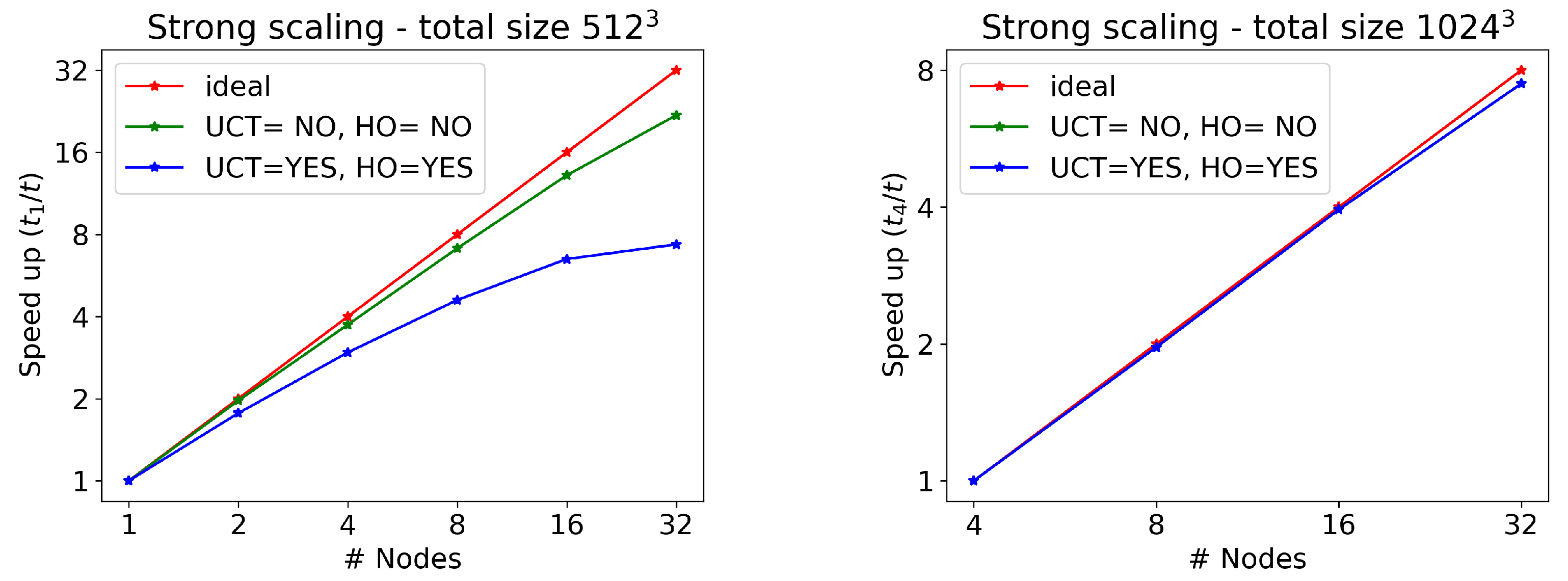
As far as scaling tests for different numbers of GPUs are concerned, we use the pre-exascale Tier-0 LEONARDO supercomputer at CINECA, equipped with four NVIDIA Ampere A100 GPUs and 64 GB of memory in every node, connected by a 2000 Gb/s internal network. We test the RMHD CPA-3D wave, now with a much larger number of cells (${512}^3$ and ${1024}^3$), without writing any output on disk and on two cases: with UCT and HO activated or not. The results are reported in

Table 1. Results for the RMHD CPA-3D wave test (using ${512}^3$ cells), on LEONARDO at CINECA (4 NVIDIA Ampere A100 GPUs per node, 4 to 128 GPUs). We report all-clock time (time to solution) in seconds and speed in iterations per second for increasing number of nodes.

CPA-3D (512${}^3$)	UCT=HO=NO		UCT=HO=YES
# Nodes	W-Time [s]	Speed [iter/s]	W-Time [s]	Speed [iter/s]
1	1735.5	1.21	1857.4	1.13
2	882.4	2.38	1050.0	2.00
4	464.6	4.52	628.7	3.34
8	243.9	8.61	403.8	5.20
16	131.7	15.95	285.7	7.35
32	79.3	26.49	252.6	8.31

and

Table 2. Results for the RMHD CPA-3D wave test (using ${1024}^3$ cells) on LEONARDO at CINECA (4 NVIDIA Ampere A100 GPUs per node, from 16 to 128 GPUs). We report all-clock time (time to solution) in seconds and speed in iterations per second for increasing number of nodes.

CPA-3D (1024${}^3$)	UCT=HO=NO		UCT=HO=YES
# Nodes	W-Time [s]	Speed [iter/s]	W-Time [s]	Speed [iter/s]
4	7188.5	0.58	7964.6	0.53
8	3654.7	1.16	4212.0	1.00
16	1820.5	2.31	2297.1	1.83
32	962.0	4.37	1374.4	3.06

, whereas the corresponding strong scaling plots (time to solution with the minimum number of nodes, divided by the time to solution for a given number of nodes) can be found in Figure 2. Note that a single node is capable of treating runs with ${512}^3$ cells, whereas when using ${1024}^3$ (more than one billion) cells, at least four nodes are needed, given that the memory per node is not sufficient.

As we can see, strong scaling is quite good when UCT and HO are not active, and the reason is that MPI communications are kept at a minimum, only needed before the main loops for computing fluxes. On the other hand, the UCT for preserving a solenoidal magnetic field and the use of the high-order version of INT and DER routines require many other MPI calls to fill in ghost cells, and the time spent in communications over pure computation can severely affect efficiency. This is confirmed by the fact that the problem is less important when increasing N, as clearly shown in Figure 2. For $N=1024$, there is an excellent scaling even when UCT=HO=YES. In order to alleviate the problem, one should try to reduce communication at the price of increasing computation. One way to achieve this would be to double the size of the ghost cell regions to be exchanged between MPI tasks (before the main loops with the calls to REC), hence computing numerical fluxes on a larger domain, so that the higher-order corrections do not require any additional update of ghost cells via MPI calls (this is true also for the UCT procedures). This procedure would be needed just once per iteration sub-step and would be applied to all variables at once.

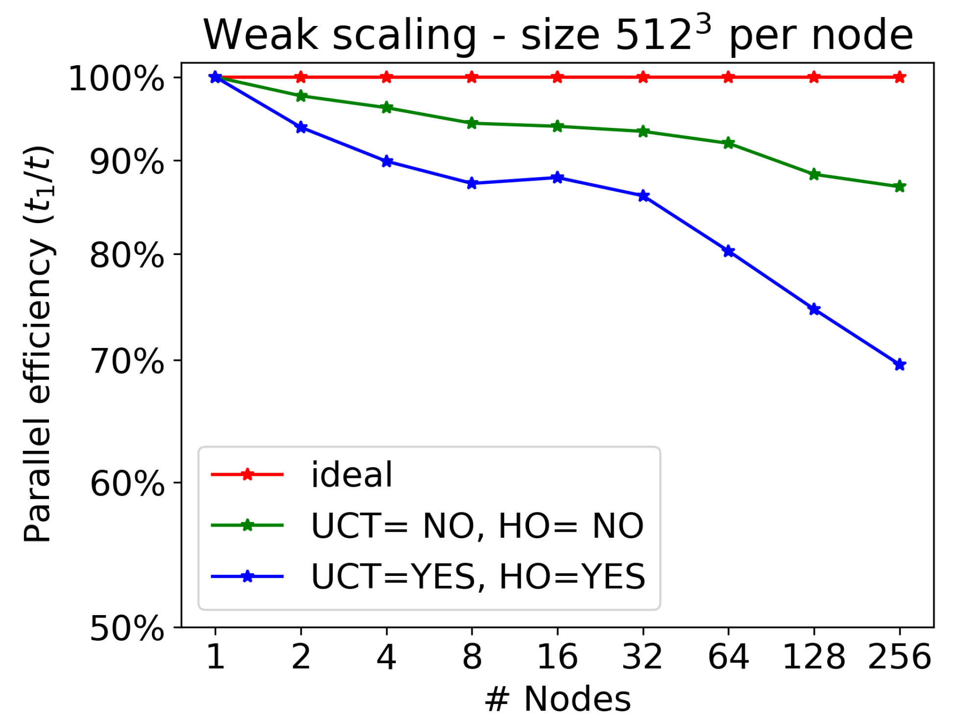
Let us now discuss weak scaling, that is, the time to solution as a function of the number of nodes (we recall that we always employ all four GPUs available per node), normalized to the case of a single node, when the number of computational cells per node is kept constant (here, we choose ${512}^3$). Results are reported in

Table 3. Results for the RMHD CPA-3D wave test (using ${512}^3$ cells per node), on LEONARDO at CINECA (4 NVIDIA Ampere A100 GPUs per node, so from 4 to 1024 GPUs). We report wall-clock time (time to solution) in seconds and speed in iterations per second for increasing number of nodes.

CPA-3D (512${}^3/$Node)	UCT=HO=NO		UCT=HO=YES
# Nodes	W-Time [s]	Speed [iter/s]	W-Time [s]	Speed [iter/s]
1	1735.5	1.21	1857.4	1.13
2	1777.3	1.18	1979.1	1.06
4	1804.0	1.16	2065.5	1.02
8	1839.7	1.14	2124.0	0.99
16	1846.8	1.14	2108.4	1.00
32	1858.7	1.13	2157.2	0.97
64	1886.8	1.11	2312.9	0.91
128	1962.0	1.07	2488.3	0.84
256	1992.8	1.05	2668.2	0.79

and displayed in Figure 3, ranging from 1 to 256 nodes, the maximum allowed for production runs on LEONARDO. The largest run, employing 256 nodes (hence 1024 GPUs) corresponds to $4096\times 4096\times 2048\simeq 34.4$ billion computational cells.

Since the timestep also changes when changing the resolution, for the present efficiency test we must maintain the number of iterations constant (we chose the one needed to complete the test on a single node). As for strong scaling, efficiency is very good in the case UCT=HO=NO, with losses kept within $10\%$, while it becomes much worse when communications are more numerous for the case UCT=HO=YES. This is just the same problem encountered for strong scaling; as discussed previously, it could be cured by passing all boundary cells at once at the cost of increasing the computational domain for each node. When this is achieved, the corresponding efficiency is expected to stay even above the actual green curve in the plot.

In absolute numbers, the peak performance for the test with ${512}^3$ cells corresponds to $1.6\times {10}^8$ cells updated each iteration per second (one node, UCT=HO=NO). If we use second-order time-stepping and linear reconstruction rather than MP5, this number rises up to $2.2\times {10}^8$. Very similar values are found by further increasing the number of cells, up to the extreme resolution of ${640}^3$ per node.

5. A Physical Application: 2D Relativistic MHD Turbulence

A perfect physical application of our accelerated version of the ECHO code is that of decaying RMHD turbulence, given that the Minkowski flat spacetime and periodic boundary conditions are involved, that is, the same numerical setup used for our scaling benchmarks with the CPA-3D wave. Here, only a high-resolution 2D problem will be presented, with fluctuations in the $x-y$ plane and a dominant uniform magnetic field $B_0$ in the perpendicular direction z (it is actually a 2.5D problem). The initial condition is that of a static and homogeneous fluid with ${\rho }_0=1$, whereas (cold) magnetization and plasma-beta parameters (as defined in [21]) are

$${\sigma }_0=B_0^2/{\rho }_0=100,{\beta }_0=2p_0/B_0^2=1,$$

(13)

so that $B_0=10,p_0=50$. The (relativistic) Alfvén and sound speeds are similar

$$v_A=\frac{B_0}{\sqrt{{\rho }_0+4p_0+B_0^2}}\simeq 0.57,c_s=\sqrt{\frac{4}{3}\frac{p_0}{{\rho }_0+4p_0}}\to \frac{1}{\sqrt{3}}\simeq 0.58,$$

(14)

where we have used $\widehat{\gamma }=4/3$, corresponding to a magnetically dominated and extremely hot plasma. To this uniform background, we add fluctuations in the perpendicular $x-y$ plane in the form of a superposition of modes at different wavelengths

$$\delta \mathit{v}=\eta v_A\sum _{k_x=0}^4\sum _{k_y=-4}^4\frac{\mathit{k}}{k}cos[\mathit{k}·\mathit{x}+{\phi }_v\left(\mathit{k}\right)]\times {\mathit{e}}_z,$$

(15)

$$\delta \mathit{B}=\eta B_0\sum _{k_x=0}^4\sum _{k_y=-4}^4\frac{\mathit{k}}{k}cos[\mathit{k}·\mathit{x}+{\phi }_B\left(\mathit{k}\right)]\times {\mathit{e}}_z.$$

(16)

Here, $\eta$ is a normalized amplitude, $\mathit{k}=(k_x,k_y)$ is the wave vector of module k, that for a square domain with $L_x=L_y=L=2\pi$ has components ranging from 1 (full wavelength) to 4, whereas ${\phi }_v\left(\mathit{k}\right)$ and ${\phi }_B\left(\mathit{k}\right)$ have random phases depending on $k_x$ and $k_y$ and different for $\mathit{v}$ and $\mathit{B}$. Fluctuations are chosen to be Alfvénic to satisfy $\nabla ·\mathbf{v}=\nabla ·\mathbf{B}=0$ and have a flat isotropized spectral radius of 4. The common normalized amplitude has been computed (a posteriori) by imposing that

$$\frac{<\left|\delta \mathit{v}\right|>}{v_A}=\frac{<\left|\delta \mathit{B}\right|>}{B_0}={\eta }_{\mathrm{rms}}=0.25,$$

(17)

where spatial averages refer to the whole 2D domain. For the present run, we employ a single node (four GPUs) of LEONARDO at CINECA and a resolution corresponding to ${4096}^2$ cells. The wall-clock time is about 100 s for the simulation time unit ($t=1$ is the light crossing time corresponding to a unit length $l=L/2\pi =1$), using the most accurate (but also slower) version of the code with UCT=HO=YES.

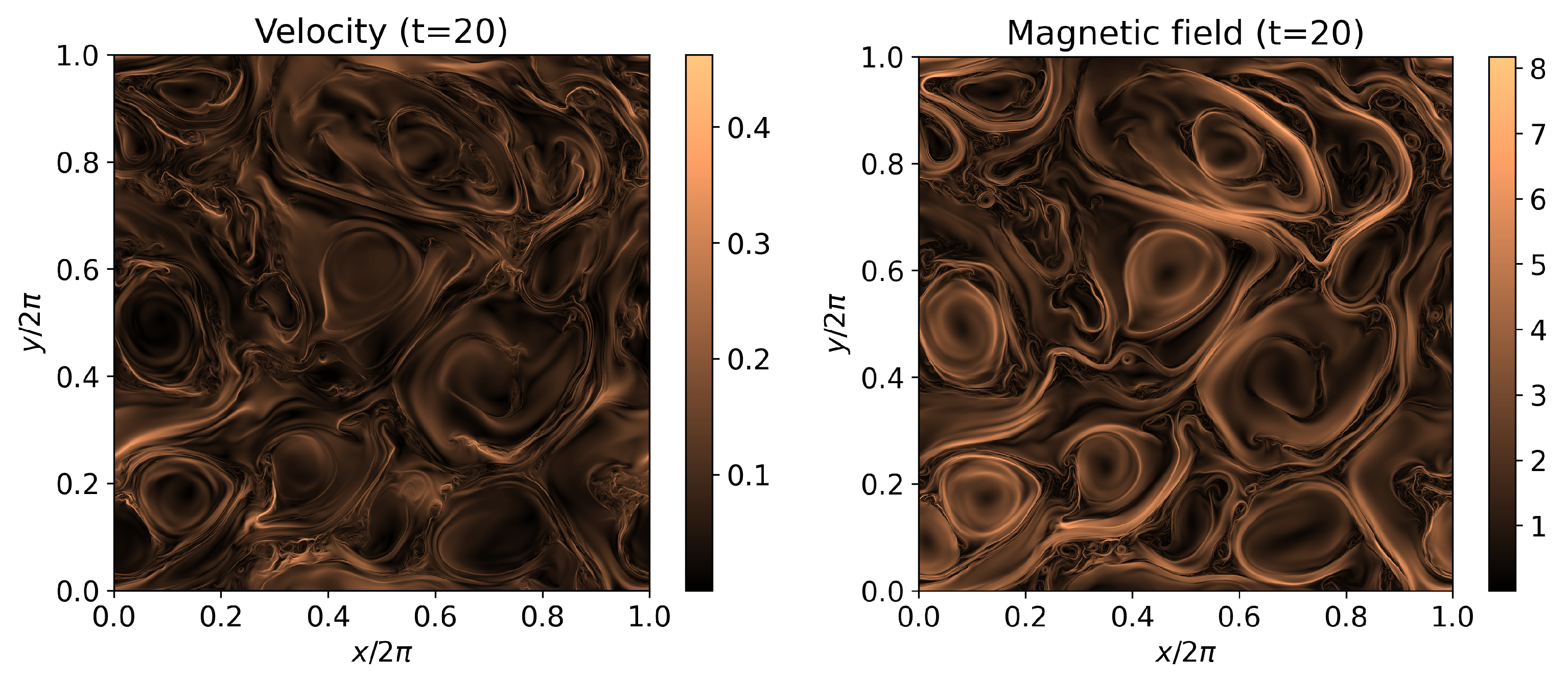
The simulation is run until $t=20$ (half an hour of wall-clock time), corresponding to few nonlinear times (i.e., the characteristic evolution time of a turbulent plasma), roughly at the peak of turbulent activity, that is, when the curve of the root-mean square of fluctuations against time reaches a maximum. The strength of fluctuations for both the velocity and magnetic field vectors are shown in Figure 4, and the turbulent nature of these fields is apparent. Vortices are now present at all scales, and energy is decaying from the large injection scale ($k\le 4$) to the dissipative one, here simply provided by the finite precision of the numerical scheme since there are no explicit velocity or magnetic dissipation terms in the RMHD equations solved here. The turbulence is sub-sonic and sub-Alfvénic, so strong shocks are not present at injection scales, even if these forms at small scales in reconnecting regions (current sheets).

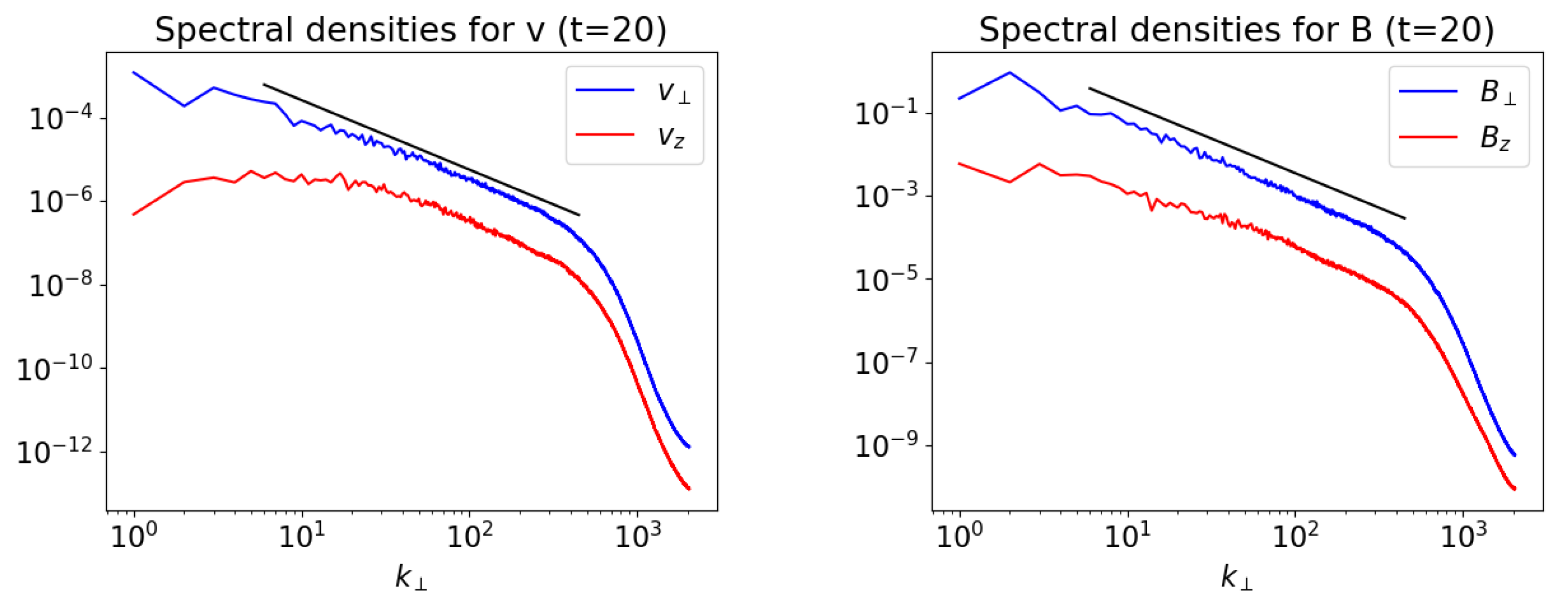
In Figure 5 we show the spectral densities for velocity and magnetic field fluctuations as a function of $k_{\perp }={(k_x^2+k_y^2)}^{1/2}$ (1D isotropized spectra). In spite of the lack of physical dissipation, there is no apparent accumulation of energy at the smallest scales, hence the numerical dissipation here is rather small. The spectra of the perpendicular components (the dominant ones) reproduce the Kolmogorov spectral slope of $-5/3$ very well for a couple of decades in $k_{\perp }$, which is a very encouraging result for a ${4096}^2$ simulation with uniform grid. We believe that the small numerical dissipation scales and the extended spectral inertial ranges are due to the use of a scheme with high (fifth-order) spatial accuracy, one of the main features of the ECHO code.

6. Conclusions

In the present paper, we have demonstrated how a state-of-the-art numerical code for relativistic magnetohydrodynamics, ECHO has been very easily ported to GPU-based systems (in particular, on NVIDIA Volta and Ampere GPUs).

Our aim was twofold, not only to accelerate the code, but also to execute this following the so-called standard language parallelism paradigm, meaning that the original code must be fully preserved by relying on just compiling options to recognize the most modern language structures (and on the addition of few directives, simply ignored by the compiler when acceleration is not needed). The version presented here is thus basically the original one, and now the very same code can run indifferently on a laptop, on multiple CPU-based cores, or on GPU accelerated devices.

Modern Fortran (the language in which ECHO was already written) provided the easiest solution to achieve our goals. The use of standard ISO Fortran structures, such as do concurrent (DC) loops and pure subroutines and functions, allows one to accelerate all the computationally intensive loops (when the order of execution is not an issue, true for many codes for fluid dynamics or MHD). Directives are provided by the widely used OpenACC API, but these are actually not necessary for data movement or loop acceleration, while we only use them for offloading the subroutines and functions invoked inside the accelerated loops (even this task would be hopefully doable by the compiler itself in the future). Full acceleration of DC loops and use of the CUDA Unified Memory address space (necessary for allocating arrays on the device and providing automatic data management between the host and the device) are simply activated by specific flags of the nvfortran compiler by NVIDIA, while message passing is ensured by the standard MPI library for domain decomposition and communication among tasks.

As far as performance on CINECA supercomputers is concerned, the code is about 16 times faster when using the four GPUs of one node on LEONARDO (with the NVIDIA compiler) compared to runs on the best performing CPU-based machine (GALILEO100 with 32 cores, $\times 4$ hyper-threading, and an Intel compiler with aggressive optimization) at the resolution of ${128}^3$. For larger sizes, and when LEONARDO is also employed for CPU multicore runs, the improvement is even higher, up to $\simeq$30 for a ${512}^3$ run. The highest peak performance using the four GPUs of a single LEONARDO node is $2.2\times {10}^8$ cells updated each iteration per second, reached at both ${512}^3$ and ${640}^3$ resolutions for the second-order version of the code. These numbers are quite important; they mean that a CPU-based simulation may require from 15 to 30 nodes to achieve the same result in the same time obtained by using just a single node employing four GPUs.

Parallel scaling is very good within a single node; otherwise, efficiency drops, unless the ratio of the time spent in computation over communication is large, and this is basically always true when GPUs are needed. The simplest version of the code, where MPI calls are at a minimum, has a very good strong scaling for ${512}^3$ cells, and a nearly ideal one for ${1024}^3$ cells. The weak scaling test, using ${512}^3$ cells per node, shows an efficiency loss of just about ∼10–15% in the range from 1 to 256 nodes (up to 1024 GPUs, corresponding to a maximum size of $4096\times 4096\times 2048\simeq 34.4$ billion cells). These performances worsen if full high order and the UCT method are both enforced, given the numerous and non-GPU-aware communications between tasks (that is among GPUs). Also, to improve both strong and weak scaling in the most complete case, we plan to enlarge the size of the halo regions of ghost cells to be exchanged among MPI tasks at the cost of increasing computations, so that message passing is performed just once per timestep in a single call for all variables. Parallel efficiency is expected to rise to above $90\%$; however, we prefer to leave this task as future work.

The code will be soon applied to the study of 3D (special) relativistic MHD turbulence; here, we have only provided an example in 2D, showing simulations of decaying Alfvénic turbulence for a strongly magnetized and relativistically hot plasma. Small-scale vortices and current sheets are ubiquitous, and two full decades of inertial range in the (isotropized) spectra with a clear Kolmogorov $-5/3$ slope, are obtained (for a resolution corresponding to ${4096}^2$ cells). Numerical dissipation only affects the finest scales and appears to be well behaved, given that no accumulation of energy at the smallest scales is visible. Since the wall-clock time taken by an Alfvén wave to cross a 3D domain is estimated to be about an hour for a resolution of ${4096}^3$ using a full allocation of 256 nodes on LEONARDO, a 3D simulation of decaying turbulence at the same resolution is expected to last just a few hours.

Moreover, as the code is already capable of working in any curved metric of general relativity, we are also ready to apply the new version of ECHO to the study of plasma surrounding compact objects, for example, disk accretion onto static and rotating black holes, extending to 3D our previous works for axisymmetric flows [7,8].

In conclusion, we deem that basically any code for fluid dynamics or MHD written in modern Fortran could be easily ported to GPUs (and heterogeneous architectures) with a minimal effort by following our guidelines; hence, we hope that our example may be useful to many other scientists and engineers. Perhaps surprisingly, it seems that the Fortran programming language, originally designed in the fifties simply for FORmula TRANslation algorithms, can still be a leading language for science and engineering software applications, even presently in the pre-exascale era. We also strongly believe that the standard language parallelism paradigm should be the path to follow in the future of HPC.