Calibration and Verification of Operation Parameters for an Array of Vectrino Profilers Configured for Turbulent Flow Field Measurement around Bridge Piers—Part II

Abstract

High-frequency velocimeters used for flow measurements during laboratory experiments allow the user to select the range for several operation parameters to set up the instrument for optimal velocity measurement. The discrepancies between velocity measurements collected with different instrument configurations can be significant, depending on the flume bed configuration and boundary conditions. The aim of this paper is to quantify the differences in flow velocity profiles measured with Acoustic Doppler Velocimeter Profilers (ADVPs) configured using a combination of profiling parameters: Ping Algorithm (PA), Transmit Pulse Size (TPS), and Cell Size (CS). Whereas in Part I of this research, the goal was to identify the optimal probe configuration for downstream measurement of the complex hydraulic structure (pier protected with riprap) based on a match of the flow rate with measurements from other instruments, in this paper, effect of distinct probe configuration on velocity profile and turbulent kinetic energy (TKE) is demonstrated. Differences between ADVPs’ configurations were analyzed through sensitivity analysis with the intention to calculate and compare any discrepancies in the velocity measurements for all the three measured velocity components: streamwise u, spanwise v and vertical w collected on two characteristic flume cross-sections. The results show that each parameter change has a significant effect on the measured values of each velocity component when compared to the Target Configuration (TC). The largest root-mean-square-error (RMSE) is observed when TPS is changed, followed by CS and PA. Absolute RMSE calculated for TPS change from 4 mm to 1 mm is, on average, 6.30 cm/s, 0.90 cm/s, and 0.82 cm/s for velocity components u, v and w, respectively. Absolute RMSE calculated for CS change from 1 mm to 4 mm is, on average, 4.49 cm/s, 0.88 cm/s, and 0.71 cm/s for velocity components u, v and w, respectively. Absolute RMSE calculated for PA change from Adaptive to Max interval is, on average, 4.04 cm/s, 0.63 cm/s, and 0.68 cm/s for velocity components u, v and w, respectively. For a change in all parameters, RMSE is greater for the cross-section downstream of the pier than for the approach cross-section: on average, 90%, 57% and 54% for a change in the PA, TPS, and CS, respectively.

1. Introduction

Acoustic Doppler Velocimeters (ADVs) are state-of-the-practice devices used for instantaneous flow measurement, ranging from point measurements to complete cross-section mapping. ADV instruments cover a wide range of applications, from flume experiments to field deployments, with accompanying firmware tailored to specific needs. For monitoring environmental flows on larger scales, Acoustic Doppler Current Profilers (ADCPs) are used, which allow for rapid cross-sectional surveys, but at the same time, cannot capture velocity data for turbulence analysis [1]. For research oriented towards turbulence, hydraulic models in scaled laboratory experiments are often used to replicate the detailed flow field for specific applications, such as structures [2,3], river restoration measures [4,5], near-wall turbulence [6], flow–vegetation interaction [7,8,9], and inside hydraulic conduits [10,11], amongst others. The usage of scaled models has several disadvantages that need to be accounted for, such as relevant data resolution [12], sidewall interference [13], or special cases of flow, such as sediment transport [14].

Reliable turbulence data, truly representing a range of scales of flow structures of interest, can be collected only if data collection instruments operate on high frequency, as do ADVs [15], or by using advanced methods, such as particle image velocimetry (PIV) [16] that allows for instantaneous velocity area mapping. Vectrino II or Vectrino profiler (Acoustic Doppler Velocimeter Profiler—ADVP) [17] is an upgraded instrument that measures instantaneous flow velocity profile, positioning it functionality-wise between the ADV and PIV techniques. 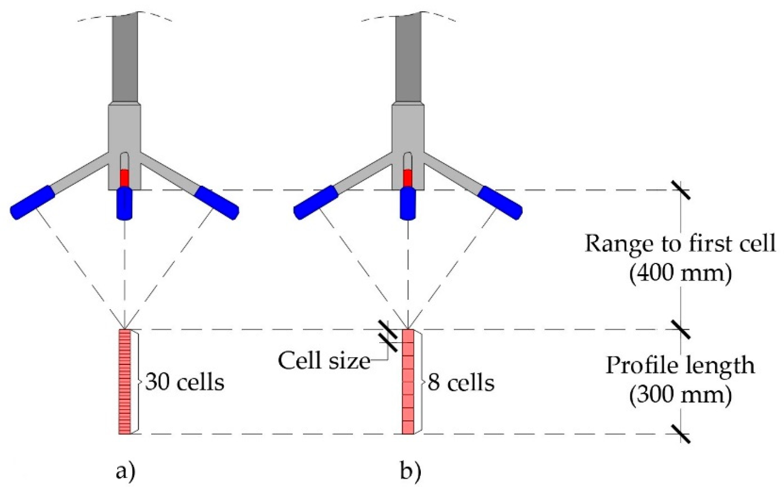ADVP (Figure 1) can measure velocity in up to 30 cells over a 45–75 mm distance from the probe with high sampling rates (≤100 Hz). Sampling cell size can be user defined in the range between 1 mm and 4 mm, with a constant diameter (6 mm). One advantage of ADVP over ADV methods is their ability to measure additional vertical velocity components, which can be used to detect noise levels in the signal [18].

Accuracy assessment for the ADVPs followed soon after its release. Zedel and Hay [19] compared the data from the two devices for flow in a turbulent jet, concluding that mean velocities, Reynolds stress, and energy spectra correspond well while noting that there is less signal to process from the ADVP since it has a smaller sampling cell size. Observations made by Leng and Chanson [20] also reveal the same pattern, reporting differences between ADV and ADVP data of an order of magnitude for instantaneous velocity fluctuations. Wren et al. [21] found that Reynolds stress from the ADVP measurements is more sensitive to the backscatter amplitude than the ones from ADV+. Similarities and differences exist when the comparison is made using PTV and PIV data. Craig et al. [22] compared the data measured by the two towed ADVPs with PIV and concluded that the mean velocity profile and log law correspond well for the two methods. Several papers [23,24,25] found that the best agreement with PTV and PIV data is near the ADVP’s “sweet spot”, while mean vertical velocities and, subsequently, TKE and Reynolds stress show significant discrepancies. The errors in the acoustic velocity measurements come from two main sources, instrument architecture and flow oscillations, in the form of Doppler noise and random spikes [26,27]. Golpira et al. [28] found that adjusting cell size and sampling frequency significantly influenced the mean flow velocity for time-averaged data and Reynolds stress near the bed for instantaneous data, consistent with the finding of Zedel and Hay [19] and Leng and Chanson [20]. They concluded that higher sampling frequency and smaller cell size improve ADV quality parameters and increase the noise variance.

The aim of this paper is to quantify the differences in flow velocity profiles measured with eight different configurations of ADVPs operation parameters through sensitivity analysis. Differences between configurations of ADVP devices were analyzed with the intention of calculating and comparing velocity measurements for all the three measured velocity components (streamwise u, spanwise v and vertical w) when the instrument is configured differently from the optimal configuration. Configurable velocity profiling parameters were Ping Algorithm (PA), Transmit Pulse Size (TPS), and Cell Size (CS). The optimal configuration against which all others were evaluated was configuration C6, defined as the most accurate for flow measurement around the bridge pier in Part I paper of this research [29], where calibration and verification of ADVPs’ operation parameters were presented. Results of calibration and verification have shown that the calculated flow rates in the flume correspond best with the pump flow and field ADCP data when ADVP is configured according to the C6 configuration with the following parameters: Ping Algorithm set to Adaptive, Transmit Pulse Size equal to 4 mm, and Cell Size of 1 mm. This research follows up to provide insight into the deviations from the true velocity that can be expected under different ADVP configurations. This research quantifies the difference of the flow velocity measured in the hydraulic flume when ADVPs’ operational parameters are adjusted, allowing the users to estimate the error introduced into the measurement.

2. Methodology

Data was collected on a scaled model of the Drava River reach around the railroad bridge in Osijek, Croatia. The physical model of the Drava River reach starting at rkm 18 + 960 (N 45.56056, E 18.70475) was constructed in an 18 m long, 0.9 m wide, and 0.9 m deep recirculating hydraulic flume in the Hydraulics laboratory under the University of Zagreb, Faculty of Civil Engineering. The bridge has two identical piers, 30 m high and 3.5 m wide, located in the main river channel with riprap scour protection installed around them, and abutments on high banks. 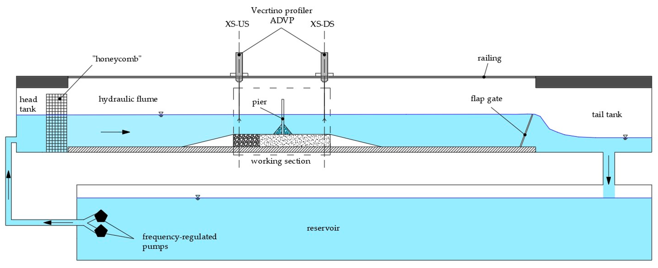This river reach was selected for analysis because it is the pilot bridge under the R3PEAT project [30], focusing on the investigation of scouring around bridge piers protected with riprap [31]. The flume bottom is lined with concrete, while the sidewalls are made of glass to allow real-time observation of the experiments. The designed working section is 3 m long, 0.4 m wide, and 0.8 m deep, with a single bridge pier placed in the model to replicate the prototype on a predefined scale. The flow conditions in the flume are driven by two frequency-regulated pumps with a maximum capacity of ~50 L/s and a hinged flap gate at the flume outlet. Water levels in the flume are monitored using two Geolux LX 80-15 10 Hz Oceanographic Radar Level sensors fitted at the inlet and outlet of the flume’s working section. The model setup consists of the river section and pier scaled according to the state-of-the-art literature [32,33,34,35,36]. Pier was modeled as a distorted scale in the vertical direction—the horizontal scale is 1:125 to the prototype, while the vertical scale is 1:11.18 with the sediment material of the prototype (ρ = 1.65 g/cm³). According to the Froude similarity principle, the velocity scale is 1:3.34 to the prototype. The flume schematic is provided in Figure 2. ADVP measurements used for analysis are the two cross-sections enclosing the working section of the hydraulic flume—upstream and downstream boundaries of the scaled river reach.

ADV instruments used for 3D flow velocity measurement are Nortek’s ADVPs, placed at the two cross-sections enclosing the flume’s working section—the upstream cross-section (XS-US) and downstream cross-section (XS-DS). XS-US is positioned at the model inlet, representing undisturbed flow conditions in the river, while XS-DS is positioned at the model outlet, representing complex flow conditions downstream of the bridge profile. Locations of the cross-sections are selected to adjust model setup to the specifics of the flume experiment. The XS-US is positioned at the upstream end of the flume’s working section where flow is contracted from the full flume width, while XS-DS is located at the position of the increased turbulence downstream of the complex pier with riprap protection. The main advantage of ADVPs over ADVs is their ability to measure velocity profile over the water column. ADVPs can measure velocity over the 30 mm range in 8–30 cells, depending on the selected cell size (1–4 mm). Additional advantage is measurement of the second vertical velocity component, allowing data quality assessment.

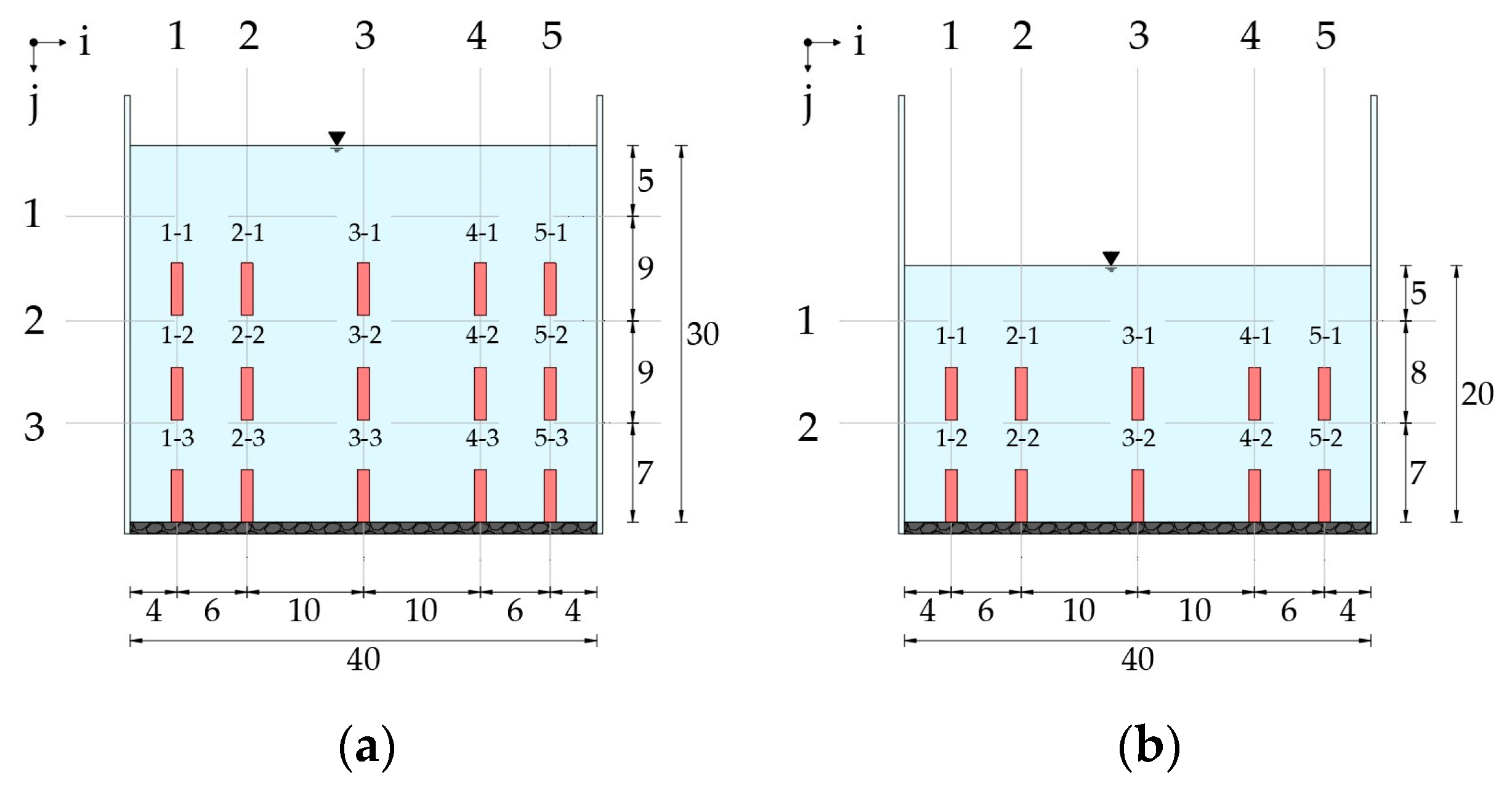
The velocity mapping approach used in this research was modeled from the standard hydrodynamic metrics found in the state-of-the-art review of hydraulics flow around bridge piers [37]. Depending on the flow depth, velocity was measured on 10 and 15 points across the cross-section to form a raster of points covering the full flow area. Points were distributed evenly over the flume width and depth; five vertical measurement axes were symmetrically placed across the flume width and two/three axes across the flow depth, as shown in Figure 3. The ADVP’s measurement locations closest to the flume sidewalls are placed as close as possible, at the distance of 4 cm to the sidewall. All measurements were made for boundary conditions combining the two flow rates (Q₁ = 20 L/s and Q₂ = 50 L/s) and two flow depths (d₁ = 30 cm and d₂ = 20 cm).

For the sensitivity analysis, the same dataset that was previously used for calibration and verification of ADVP operation parameters was utilized. Velocity data were collected with a sampling frequency of 100 Hz [22,38,39] and averaged over the entire sampling duration, ≥60 s [37,40,41]. Duration of the measurement is defined by the number of samples that are required for data processing, meaning that the duration of the measurement is dependent of the instrument’s operation frequency. Larger number of the obtained samples allow for higher statistical moments to be calculated, while first and second statistical moments of velocity components can be calculated with reduced sampling. Chanson et al. 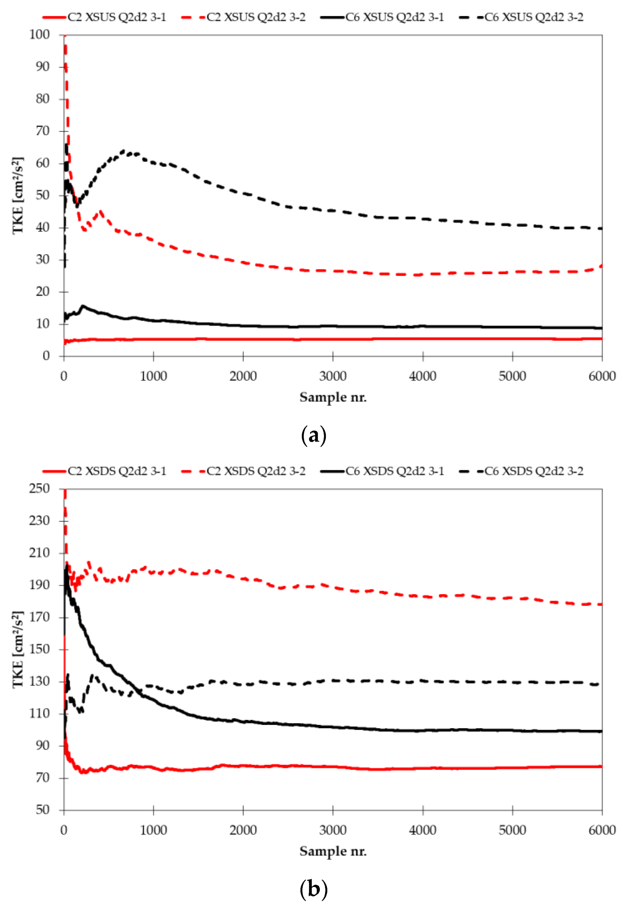[42] recommend sampling at 50,000 and 5000 for higher and lower statistical moments, respectively, while some studies report that turbulence can be estimated with even lower number of samples, e.g., 3000 [43], and 2250 [44], or that cumulative moving averages the Reynolds shear stress stabilize under 60 s [28]. Cumulative average of TKE calculated for two distinct flow conditions (Q1d1 and Q2d2) is given in the Appendix F. Cumulative average of TKE is presented for the flume mid-section, for each probe configuration and each flow conditions. It can be seen that the TKE stabilizes within the 6000 measured samples for both XS-US and XS-DS.

Data quality was ensured through de-spiking and noise reduction, deploying the methods common in the research field [45,46,47,48,49]. The ADVP’s operation parameters used for the measurements are configurable in the data collection software (Vectrino profiler v1.37, available from https://www.nortekgroup.com/software, accessed on 23 June 2023). Configurable parameters are Ping Algorithm which can be set as Max interval, Min interval or Adaptive, Cell Size and Transmit Pulse Size, which can be set from 1 mm to 4 mm. In the initial phase of the experiments, it was found that the Min interval PA gave randomly scattered results and had too low velocities. For this reason, the PA was only tested for the Adaptive and Max interval settings. For each PA setting, the TPS and CS were varied between their maximum and minimum values, 1 and 4 mm, respectively. This resulted in a total of 8 ADVP configurations (

Table 1. Configuration of ADVP’s operation parameters used for analysis.

Configuration	Ping Algorithm	Cell Size [mm]	Transmit Pulse Size [mm]
C1	Max interval	1	1
C2			4
C3		4	1
C4			4
C5	Adaptive	1	1
C6			4
C7		4	1
C8			4

) and 32 experimental runs (a combination of 8 ADVP configurations with 4 distinctive boundary conditions).

A sensitivity analysis is performed to determine the influence of different parameters on the measured velocity data. During the calibration and verification procedure [29], configuration C6 (PA set to Adaptive, CS set to 1 mm, and TPS set to 4 mm) proved to be the best suited for flow field measurements in the model of bridge pier protected with riprap that was described in detail in Part I of this research. For that reason, configuration C6 will be referred to as the Target Configuration (TC). TC was compared with each of the ADVP configurations that share the same 2 of 3 changeable operation parameters and differ only in the value of the third parameter. The three configurations that are in this way comparable to TC (C2, C5 and C8) are hereafter referred to as the Analogous Configurations (ACs). Each of the ACs, in comparison to TC, presents the specific parameter change: PA, TPS, and CS for C2, C5, and C8, respectively. For configurations with exactly the same number of cells as TC, C2 and C5, the analysis is performed for each cell, while for configuration C8 which has a larger CS, the velocity measurements obtained with the TC are averaged for the 1 mm cells occupying the same flow space as the 4 mm cells in C8 (Figure 4).

A sensitivity analysis of the instrument configurations compared to the TC is performed using the root-mean-square-error (RMSE) analysis commonly used for velocimeter performance assessment [50,51]. The RMSE gives the standard deviation of the difference between the predictions and the true values. The RMSE indicates the magnitude of the errors and is expressed in the same unit as the dataset. The lower the RMSE, the smaller the deviation from the true value [52]. The general equation for RMSE is given as follows:

$$RMSE=\sqrt{\frac{1}{n}\sum _{i=1}^n{\left(y_i-\widehat{y_i}\right)}^2} ,$$

(1)

where, $\widehat{{\mathrm{y}}_i}$= the true value of a single point, y_i = the prediction value of a single point, n = the number of observed points, and i = the counting index.

In this study, the results of velocity measurements were compared between TC and each AC on a measurement cell basis across all point measurements. RMSE values are calculated separately for an entire cross-section from time-averaged single-cell data for each velocity component. In this context, the RMSE represents the difference between TC and AC velocities for the entire cross-section, i.e., it provides an error estimate of how much the measured velocities deviate from the true TC values when one operational parameter is changed. RMSE is calculated as follows for each velocity component and turbulent kinetic energy (TKE) over the entire cross-section:

$${\mathit{RMSE}}_u=\sum _i^n\sum _j^m\sqrt{\frac{{\left(u_{AC,ij}-u_{TC,ij}\right)}^2}{m·n}} ,$$

(2)

$${\mathit{RMSE}}_v=\sum _i^n\sum _j^m\sqrt{\frac{{\left(v_{AC,ij}-v_{TC,ij}\right)}^2}{m·n}} ,$$

(3)

$${\mathit{RMSE}}_w=\sum _i^n\sum _j^m\sqrt{\frac{{\left(w_{AC,ij}-w_{TC,ij}\right)}^2}{m·n}} ,$$

(4)

$${\mathit{RMSE}}_{TKE}=\sum _i^n\sum _j^m\sqrt{\frac{{\left({TKE}_{AC,ij}-{TKE}_{TC,ij}\right)}^2}{m·n}} ,$$

(5)

where, u_TC,ij, v_TC,ij, w_TC,ij = velocity components u, v, w measured in a single cell for TC, respectively; u_AC,ij, v_AC,ij, w_AC,ij = velocity components u, v, w measured in a single cell for AC, respectively; TKE_TC,ij = turbulent kinetic energy calculated for a single cell for TC; TKE_AC,ij = turbulent kinetic energy calculated for a single cell for AC; m = number of measurement cells in vertical direction and n = number of measurement cells in horizontal direction.

3. Results

The RMSE values of time-averaged velocities quantify the deviation from the TC for all the ACs under the four combinations of flow rate and flow depth. Calculating the RMSE allows evaluation of the sensitivity of measured velocities to change in ADVP configuration. Calculated RMSE for varying PA (deviation between C2 and TC), CS (deviation between C8 and TC), and TPS (deviation between C5 and TC) are presented in

Table 2. Calculated RMSE between configurations C2 and TC data—f(PA).

Cross-Section	Boundary Conditions	RMSEu [cm/s]	RMSEv [cm/s]	RMSEw [cm/s]	$\overline{\mathbf{RMSE}}$ [cm/s]	RMSETKE [cm2/s2]
XS-US	Q1d1	1.124	0.165	0.285	0.524	3.43
	Q1d2	2.190	0.229	0.247	0.889	2.55
	Q2d1	4.059	0.830	0.703	1.864	5.85
	Q2d2	3.483	0.787	0.616	1.629	40.04
XS-DS	Q1d1	1.998	0.277	0.413	0.896	2.42
	Q1d2	4.480	0.490	0.834	1.934	19.05
	Q2d1	6.473	0.673	1.409	2.852	13.40
	Q2d2	8.498	1.555	0.922	3.658	74.86

,

Table 3. Calculated RMSE between configurations C8 and TC data—f(CS).

Cross-Section	Boundary Conditions	RMSEu [cm/s]	RMSEv [cm/s]	RMSEw [cm/s]	$\overline{\mathbf{RMSE}}$ [cm/s]	RMSETKE [cm2/s2]
XS-US	Q1d1	1.002	0.344	0.348	0.565	2.68
	Q1d2	3.359	0.575	0.482	1.472	23.02
	Q2d1	2.922	2.413	0.803	2.046	5.66
	Q2d2	5.323	0.915	0.644	2.294	37.23
XS-DS	Q1d1	2.588	0.243	0.404	1.078	2.24
	Q1d2	4.325	0.383	0.723	1.811	16.85
	Q2d1	7.359	0.717	1.175	3.083	11.16
	Q2d2	9.058	1.452	1.111	3.874	86.36

, and

Table 4. Calculated RMSE between configurations C5 and TC data—f(TPS).

Cross-Section	Boundary Conditions	RMSEu [cm/s]	RMSEv [cm/s]	RMSEw [cm/s]	$\overline{\mathbf{RMSE}}$ [cm/s]	RMSETKE [cm2/s2]
XS-US	Q1d1	2.562	0.271	0.519	1.117	3.77
	Q1d2	4.004	0.345	0.422	1.590	3.22
	Q2d1	6.607	2.239	0.781	3.209	5.80
	Q2d2	5.112	1.281	0.778	2.391	43.42
XS-DS	Q1d1	2.209	0.240	0.456	0.968	2.37
	Q1d2	5.628	0.587	0.890	2.369	18.32
	Q2d1	7.776	1.146	1.538	3.487	15.85
	Q2d2	16.498	1.086	1.149	6.244	98.77

, respectively.

When RMSE is calculated for PA change from Adaptive to Max interval (Table 2), it is observed that RMSE is consistently higher on the XS-DS than on the XS-US; 92% on average. The largest difference is observed for velocity component w (108%), closely followed by u (96%), while the RMSE increase for the v component is not as noticeable (65%). The only exception is the v component for flow conditions Q2d1 when RMSE at XS-DS is lower than XS-US (19%). A significant RMSE increase is observed for each cross-section when the flow rate is increased from Q₁ to Q₂ while retaining the same flow depth: for both XS-US and XS-DS, RMSE increase is similar, on average, 256% and 218% for flow depth d₁ at XS-US and XS-DS, respectively, and 83% and 89% for flow depth d₂ at XS-US and XS-DS, respectively. Trend of RMSE change for TKE closely resembles the one observed for mean flow velocity: increase in flow velocity through either increased flow rate (Q₁ -> Q₂) or reduced flow depth (d₁ -> d₂) is followed by the increase in RMSE_TKE. The deviation from this trend is observed for XS-US under Q₁, when RMSE reduces with lowering of the flow depth (by 24%). As expected, RMSE_TKE for XS-DS is higher than for XS-US when compared under the same hydraulic conditions for all conditions, except the one with the smallest mean velocity (29% decrease for Q1d1). For higher velocity conditions, RMSE_TKE for XS-DS is higher than for XS-US, by up to 550% (for Q1d2).

When RMSE is calculated for CS change from 1 mm to 4 mm (Table 3), the absolute RMSE values are greater than the change in PA but lower than those for the change in TPS. The relative differences between the two cross-sections and flow conditions are similar to the change in TPS. For this AC, the RMSE is consistently higher at XS-DS than the XS-US for velocity components u (102% on average) and w (46% on average) under all flow conditions. RMSE for the v component is consistently lower for the XS-DS than for the XS-US (73% on average). The largest difference is observed for velocity component u (94%), closely followed by w (85%). RMSE for the v component is generally lower for XS-DS than for the XS-US (44% on average), except for flow conditions Q2d2, when a 59% increase is observed downstream. A significant RMSE increase is observed for each cross-section when the flow rate increases from Q₁ to Q₂ while retaining the same flow depth. For both XS-US and XS-DS, the RMSE increase is similarly greater for larger flow depth: 262% and 56%, on average, for XS-US at flow depth d₁ and d₂, respectively, and 186% and 114%, on average, for XS-DS at flow depth d₁ and d₂, respectively. As in the previous case, RMSE for TKE increases with mean flow velocity increase. However, different trend is observed for when RMSE_TKE is compared for XS-DS and XS-US under lower flow rate. For Q1d1 and Q1d2 conditions, RMSE_TKE is lower for XS-DS than for XS-US as a result of lower RMSE_v (18% and 26% for Q1d1 and Q1d2, respectively). Under the higher flow rate, RMSE_TKE for XS-DS is almost more than double of that for XS-US (196% and 132% for Q1d1 and Q1d2, respectively).

When RMSE is calculated for TPS change from 4 mm to 1 mm (Table 4), the absolute RMSE increases compared to PA change, but relative differences between the two cross-sections and flow conditions are reduced. In this case, the RMSE is lower at XS-DS than on the XS-US for all velocity components under the flow condition Q1d1 (13% on average), while it is consistently higher at the XS-DS than at the XS-US for the rest flow conditions; 73% on average. The largest difference is observed for velocity component u (94%), closely followed by w (85%). RMSE for the v component is generally lower for XS-DS than for the XS-US (25% on average), except for flow condition Q1d2 when a 70% increase is observed downstream. A significant RMSE increase is observed for each cross-section when the flow rate increases from Q₁ to Q₂ while retaining the same flow depth. XS-US and XS-DS RMSE increases are similarly greater for larger flow depth: 187% and 50%, on average, for XS-US at flow depth d₁ and d₂, respectively, and 260% and 164%, on average, for XS-DS at flow depth d₁ and d₂, respectively. Change in TPS parameter has the same influence on the RMSE_TKE as the change in PA: RMSE_TKE for XS-DS is higher than for XS-US when compared under the same hydraulic conditions for all conditions, except the one with the smallest mean velocity (37% decrease for Q1d1). For higher velocity conditions, RMSE_TKE for XS-DS is higher than for XS-US, by up to 471% for Q1d2. Increase in flow velocity is followed by the increase in RMSE_TKE. For all cases, apart from XS-US under Q₁, RMSE reduces with the lowering of flow depth (by 16%).

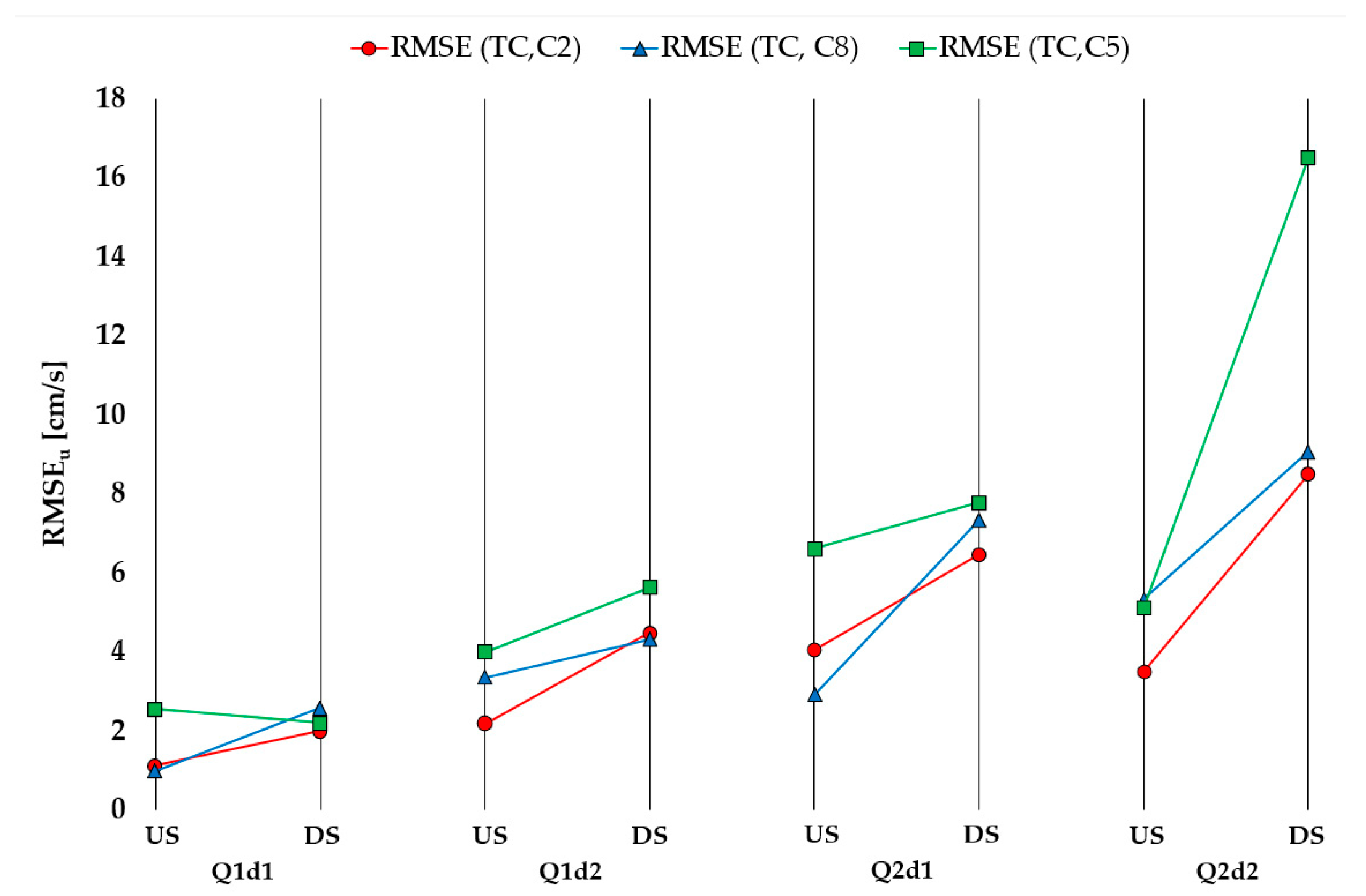
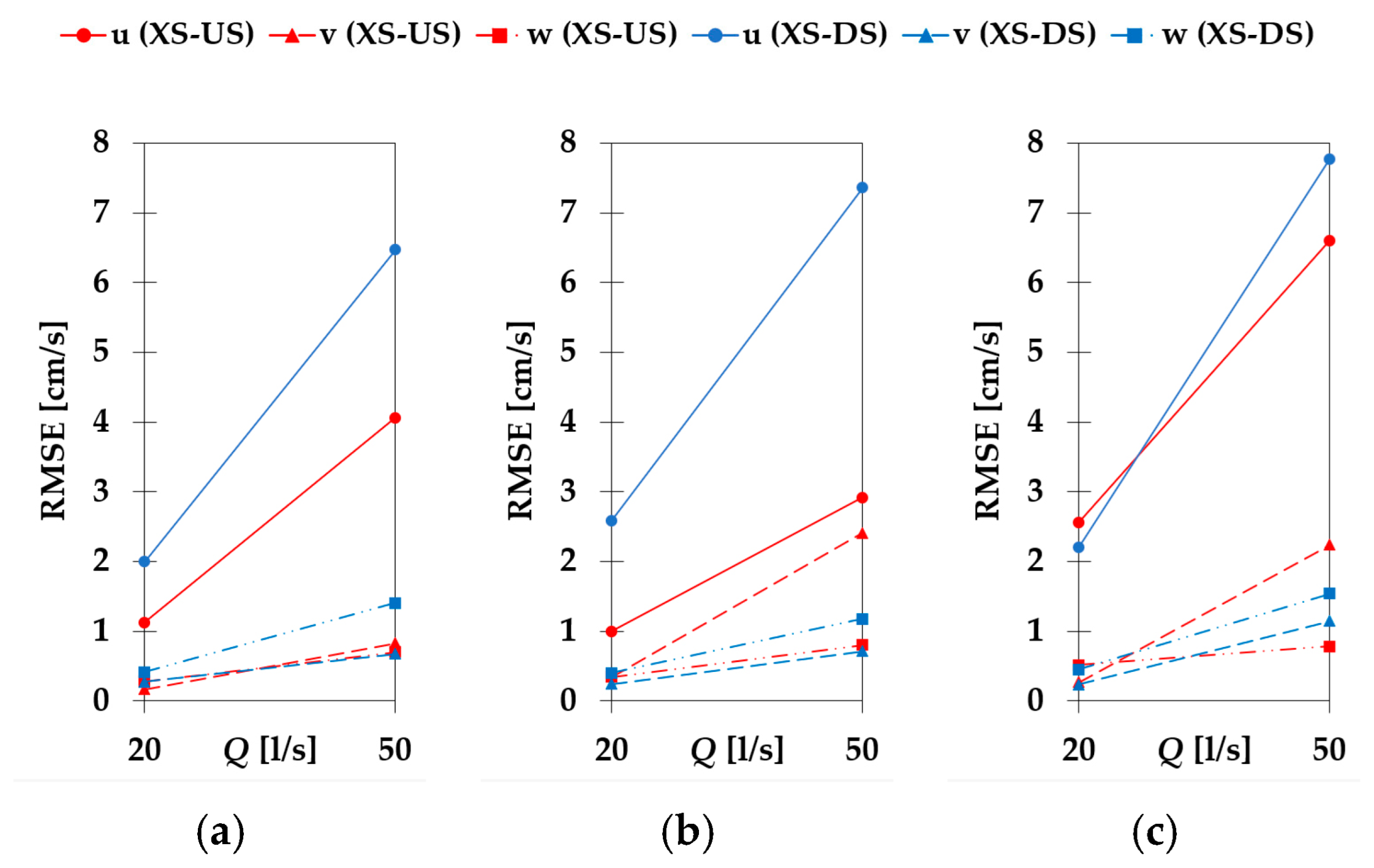
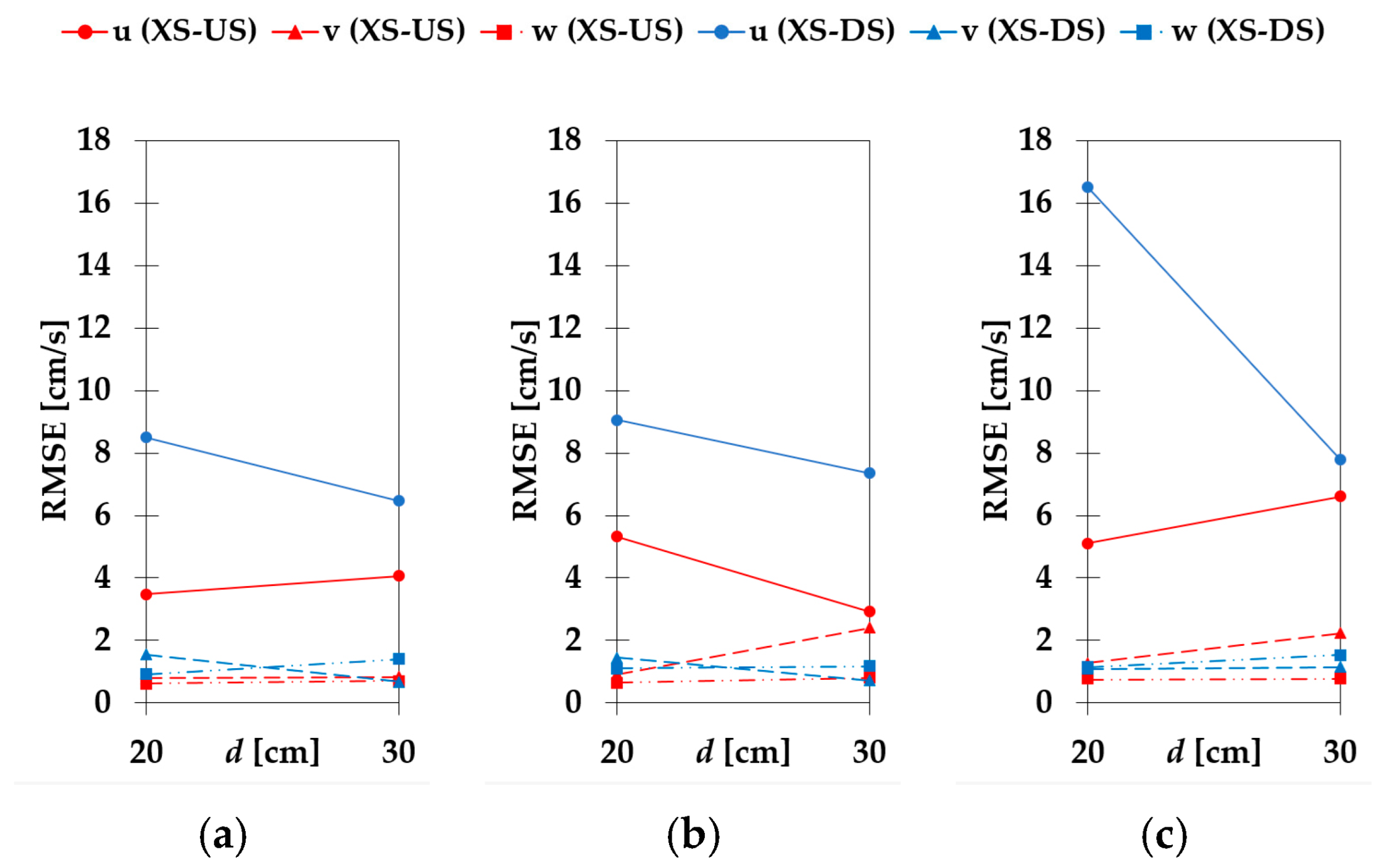
Considering all three AC configurations, the largest absolute RMSE values are calculated for the velocity component u (Figure 5). Comparing velocities measured using the AC configurations with the velocities measured using TC, the largest RMSE is observed when TPS is changed, followed by CS and PA. Absolute RMSE calculated for TPS change from 4 mm to 1 mm is, on average, 6.30 cm/s, 0.90 cm/s, and 0.82 cm/s for velocity components u, v and w, respectively. Absolute RMSE calculated for CS change from 1 mm to 4 mm is, on average, 4.49 cm/s, 0.88 cm/s, and 0.71 cm/s for velocity components u, v and w, respectively. Absolute RMSE calculated for PA change from Adaptive to Max interval is, on average, 4.04 cm/s, 0.63 cm/s, and 0.68 cm/s for velocity components u, v and w, respectively. The u velocity component has expectedly highest RMSE than the other two components, while there is no significant difference between the v and w components. At the XS-US, the average RMSE is always higher for v than w for change in PA, TPS and CS: 0.50 > 0.46 cm/s, 1.03 > 0.63 cm/s, and 1.06 > 0.57 cm/s, respectively. On the other hand, XS-DS has the opposite trend: average RMSE is always lower for v than for w; 0.75 < 0.89 cm/s, 0.76 < 1.01 cm/s, and 0.70 < 0.85 cm/s for change in PA, TPS and CS, respectively.

For the XS-US, the RMSE is largest under the flow condition Q2d1 (combination of the highest flow rate and flow depth). For the XS-DS, RMSE is the largest under the flow condition Q2d2 (combination of the highest flow rate and the lowest flow depth), resulting in the highest flow velocity. Figures (Figure 5 and other following below) are arranged in a way that mean flow velocity increases from left to right (V_Q1d1 < V_Q1d2 < V_Q2d1 < V_Q2d2). It can be observed that for both cross-sections, RMSE increases with mean flow velocity, with an exception of XS-US where RMSE trend is broken with a reduction of Q2d2 compared to Q2d1. The RMSE values are higher at the XS-US than at the XS-DS for the same flow conditions, which is expected since XS-DS is positioned in a turbulent flow downstream of the bridge pier, which may cause a higher sensitivity of the ADVP probe, while XS-US is positioned in the approach section of the flow. The u velocities are shown to be most sensitive to the change in the TPS and least sensitive to the change in the PA.

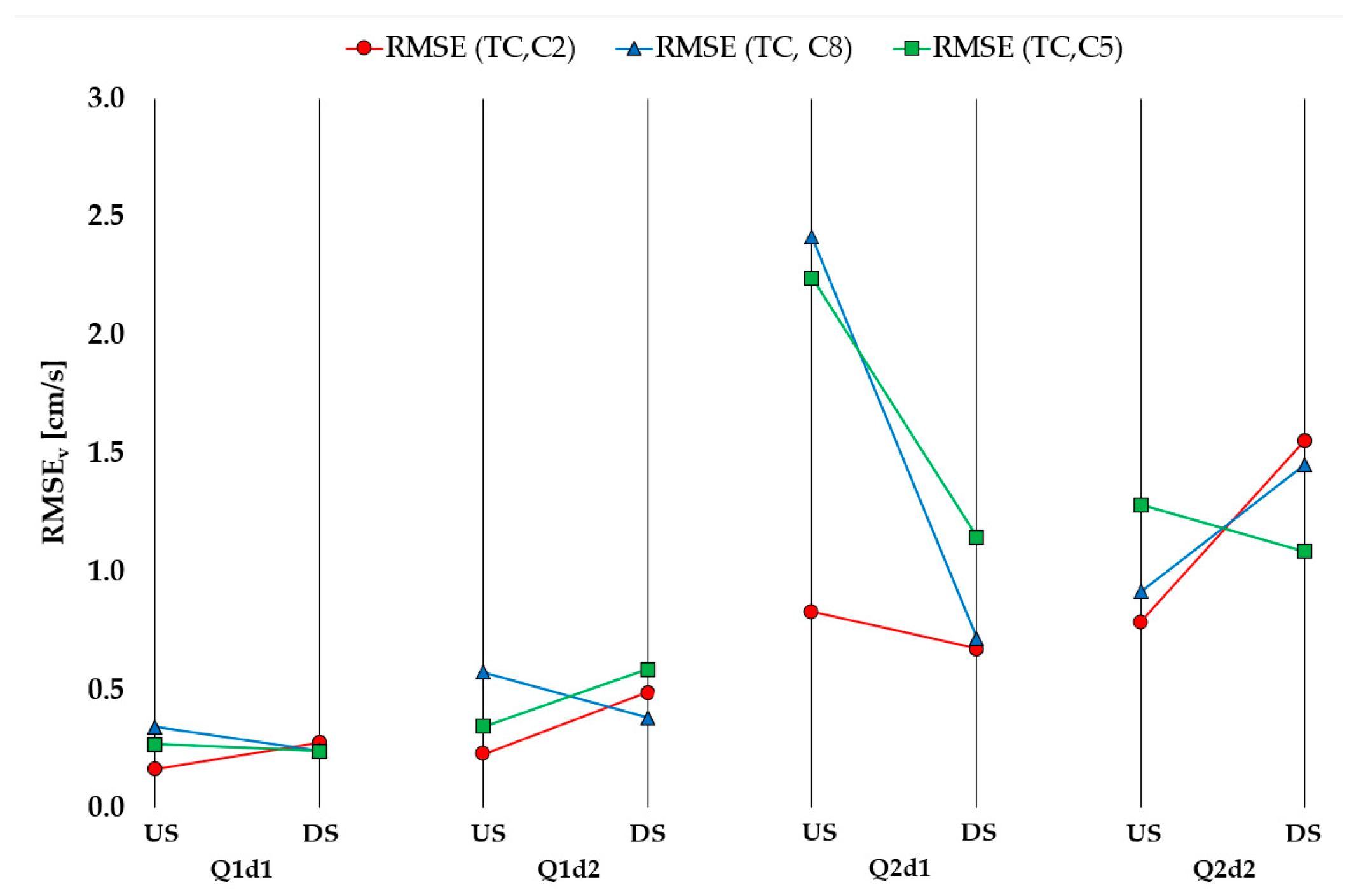
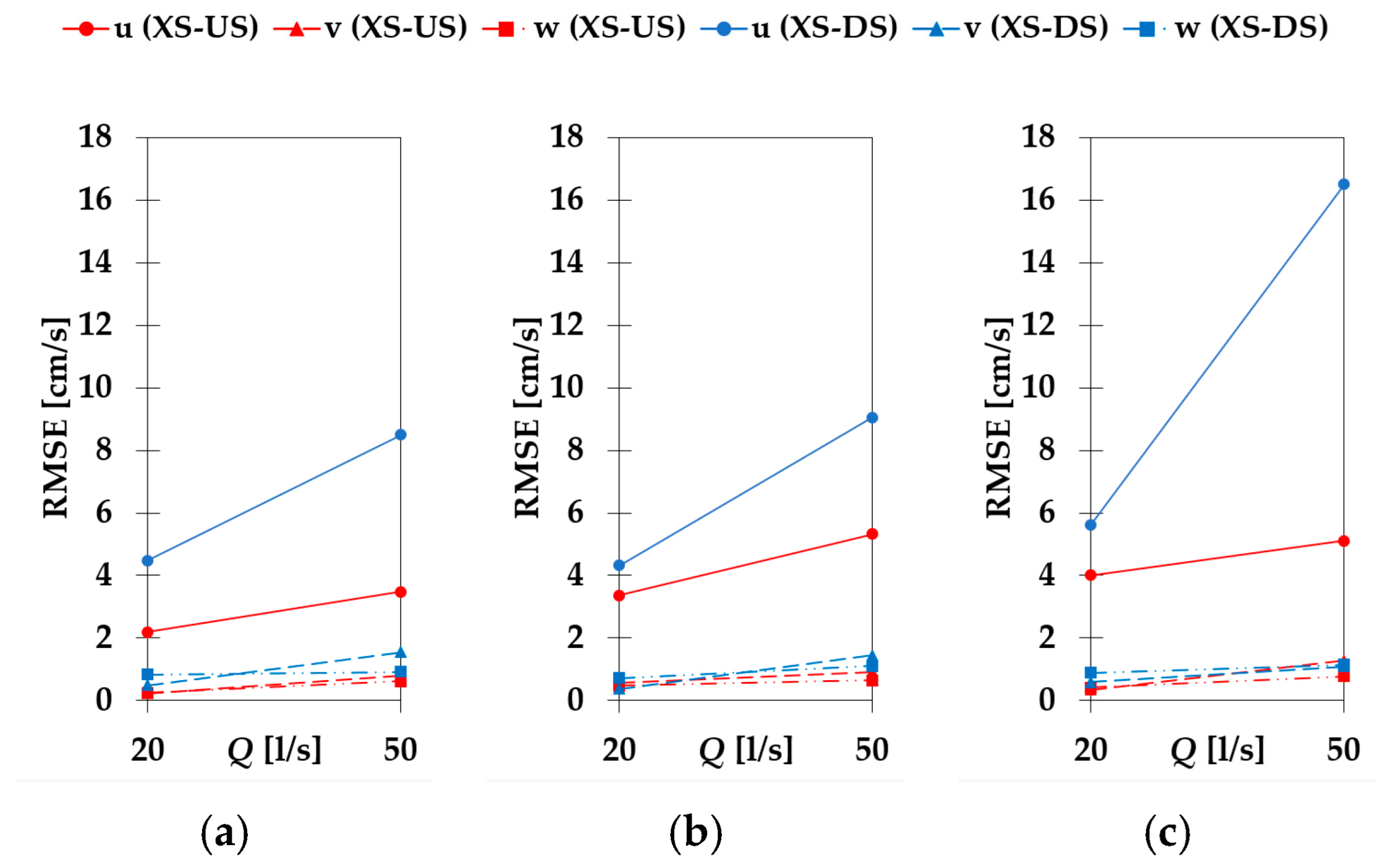
The sensitivity of the velocity component v is similar to the u components as the v velocities are shown to be most sensitive to the change in the TPS and least sensitive to the change in the PA and CS (Figure 6). For the XS-DS, RMSE is the largest under the flow condition Q2d2 for configuration C2, while for configurations C8 and C5, it is largest at Q2d1. For the XS-US, the RMSE is largest under the flow condition Q2d1 for all three configurations. The general trend of RMSE increase with the increase in the mean flow velocity is present for velocity component u, with an exception of XS-US for Q2d1 where abrupt increase in RMSE is present for C5 and C8, and slightly for C2.

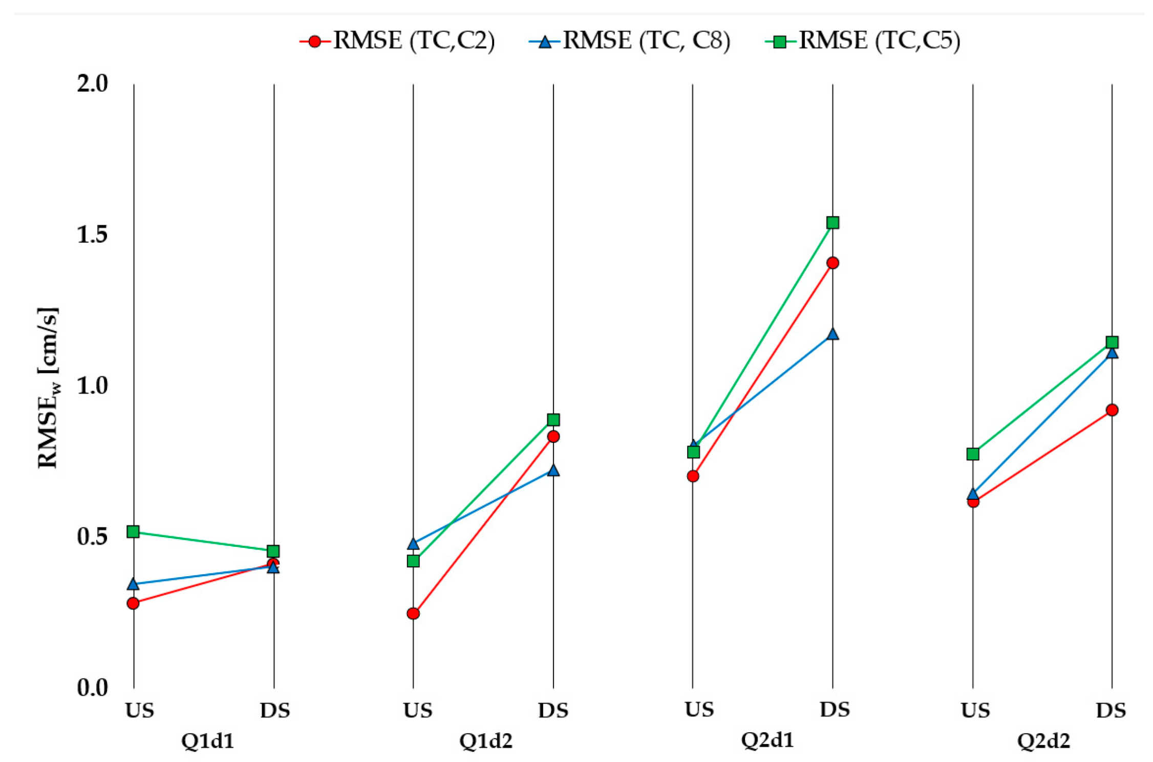
An increasing trend for the velocity component w is observed in RMSE for the XS-DS compared to the XS-US (Figure 7). The sensitivity of the velocity component w is similar to the u and v components, as the w velocities are shown to be most sensitive for the change in the TPS and least sensitive to the change in the PA and CS. The largest RMSE values for all three configurations can also be found at XS-DS for the flow condition Q2d1. For both XS-US and XS-DS, the RMSE values for Q2d1 are larger than for Q2d2, expanding on the trend observed for velocity components u and v. Additionally, slight decrease in the RMSE is present for XS-US under the flow Q1d2 and configurations C5 and C8 when compared to the overall trend.

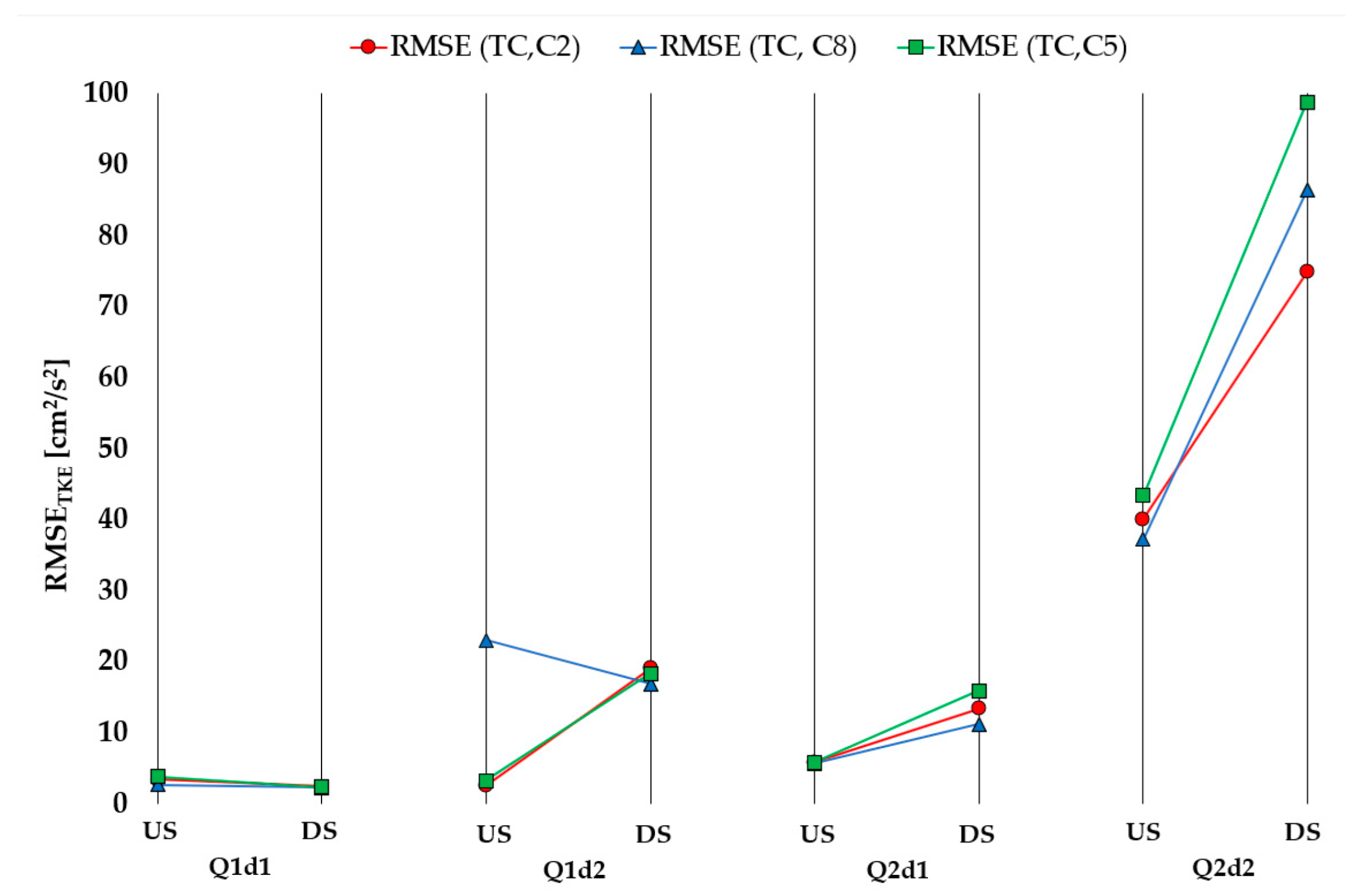
RMSE trend of TKE (Figure 8) resembles the one of the velocity components in a way that general increase in RMSE with increased mean flow velocity is present. However, the differences for RMSE below the largest flow velocity (Q2d2) are low for both velocity increase and configuration change (<0.23 cm²/s² compared to >0.37 cm²/s² for Q2d2). The flow combination of highest flow rate and flow depth (Q2d1) shows RMSE deviation from trend on XS-DS for all changes in all the configurations and on the XS-US for change in the CS. Abrupt increase in mean flow velocity (Q1d2 to Q2d2) results in greatest RMSE increase where similarity with velocity RMSE is evident through RMSE increasing for configurations from C2, C8 to C5, confirming that measurements are most sensitive to change in TPS, and least sensitive to change in PA.

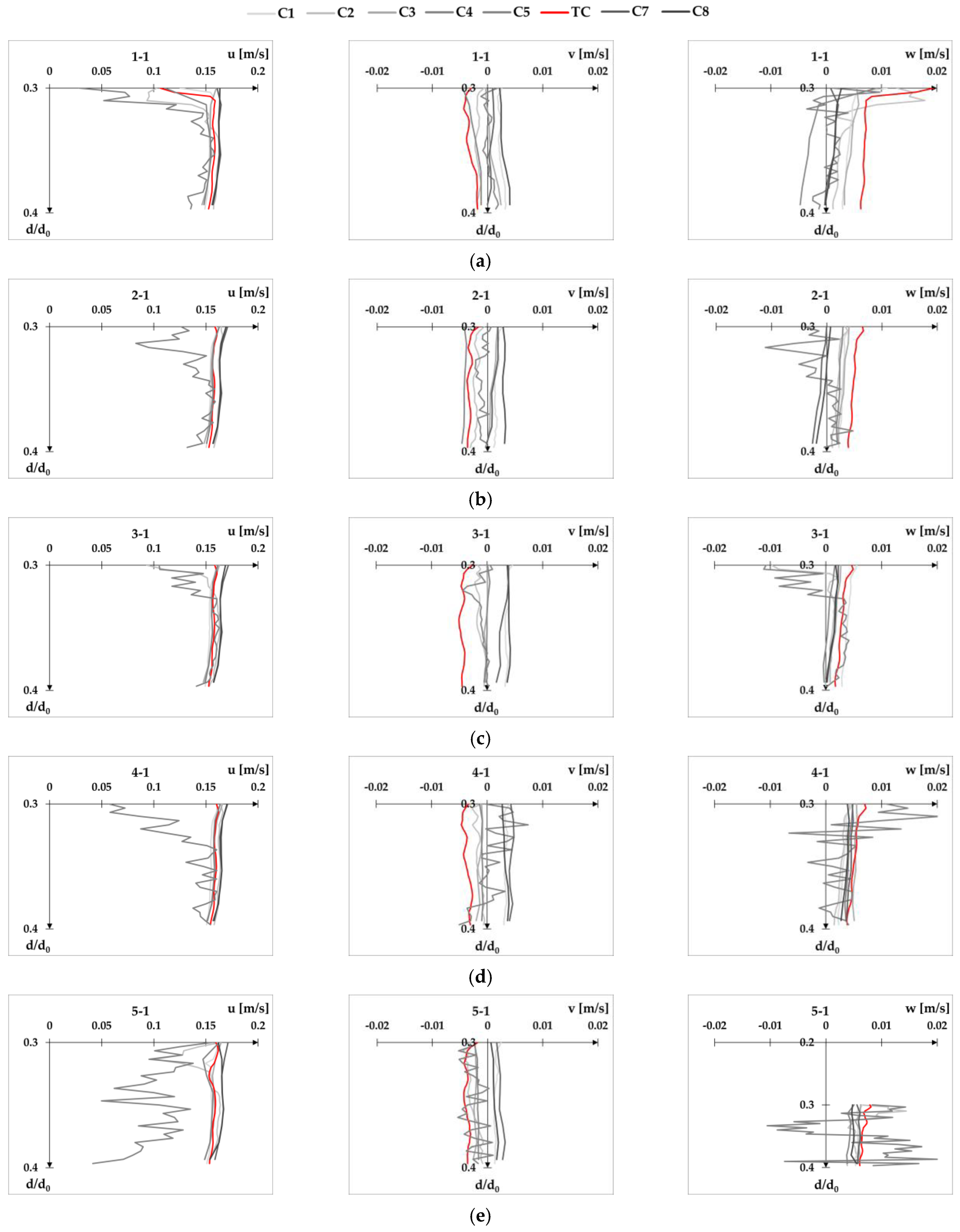
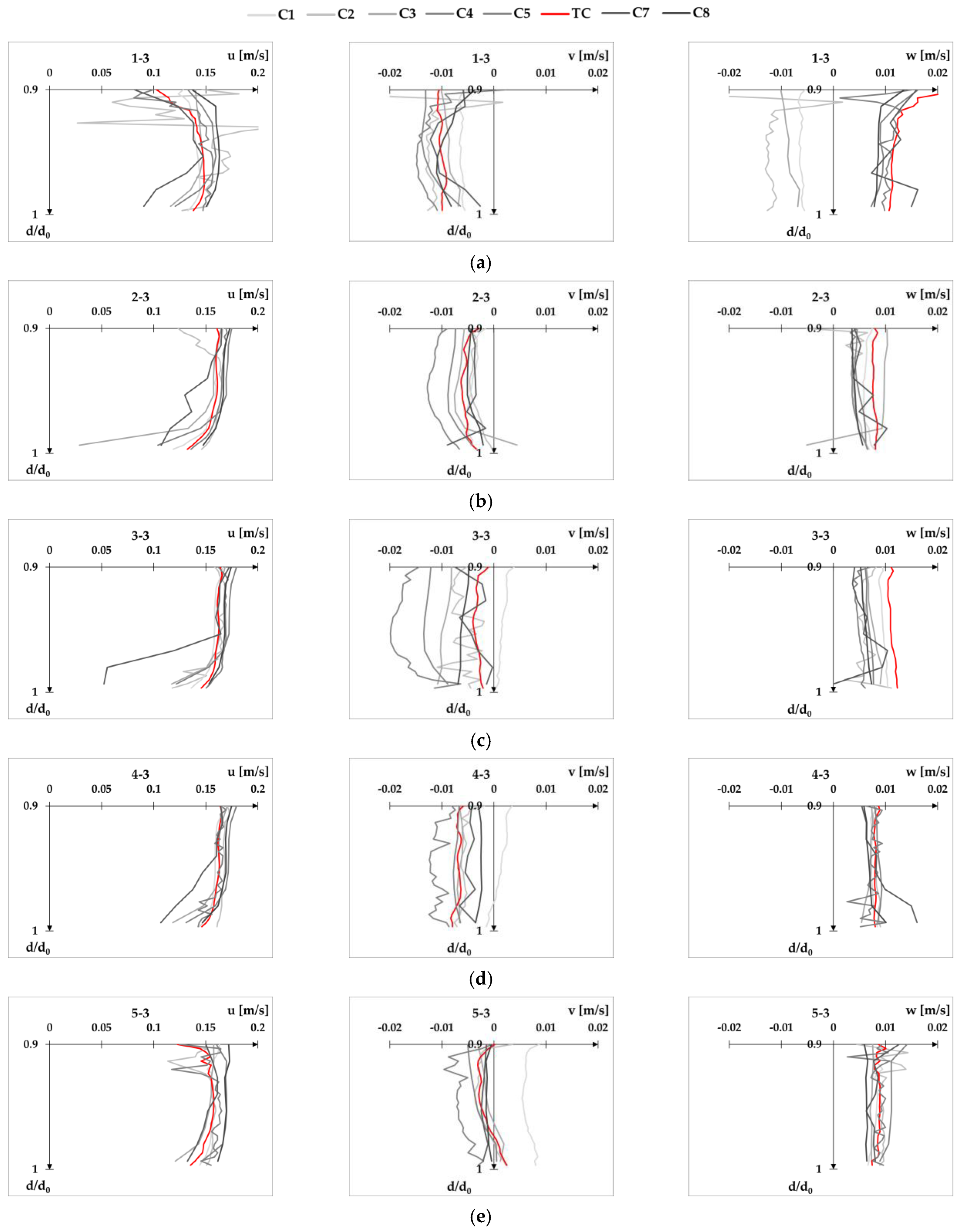
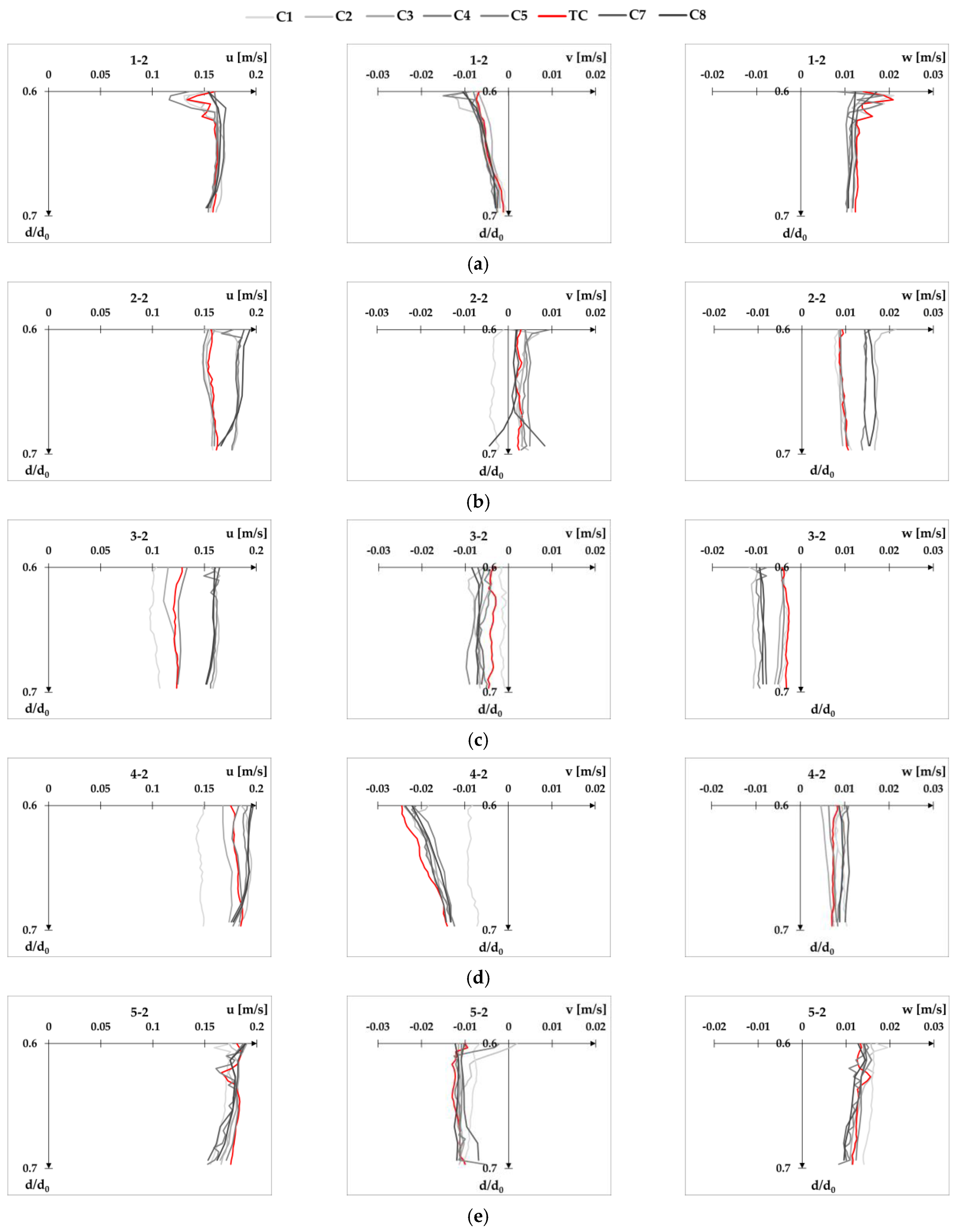
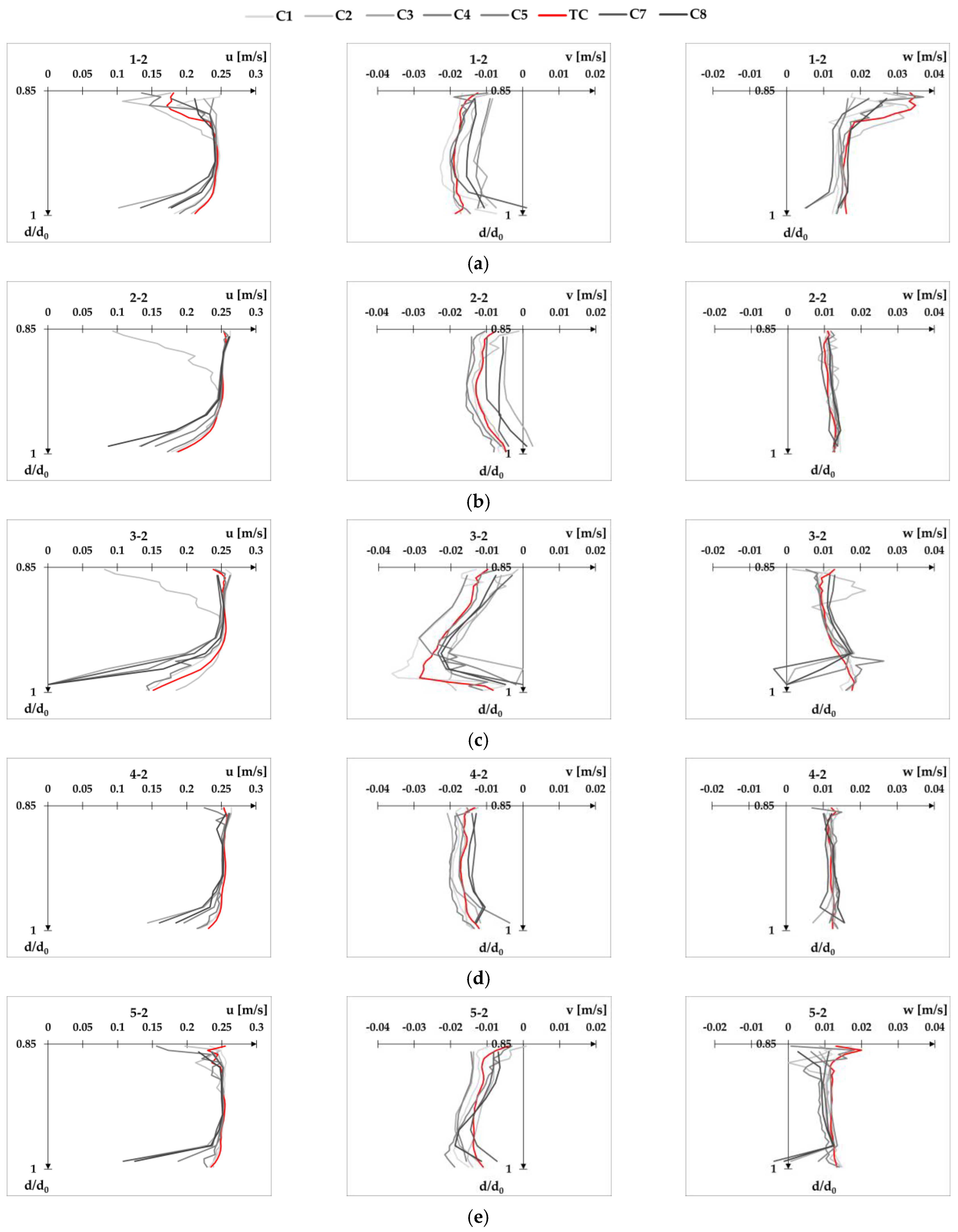
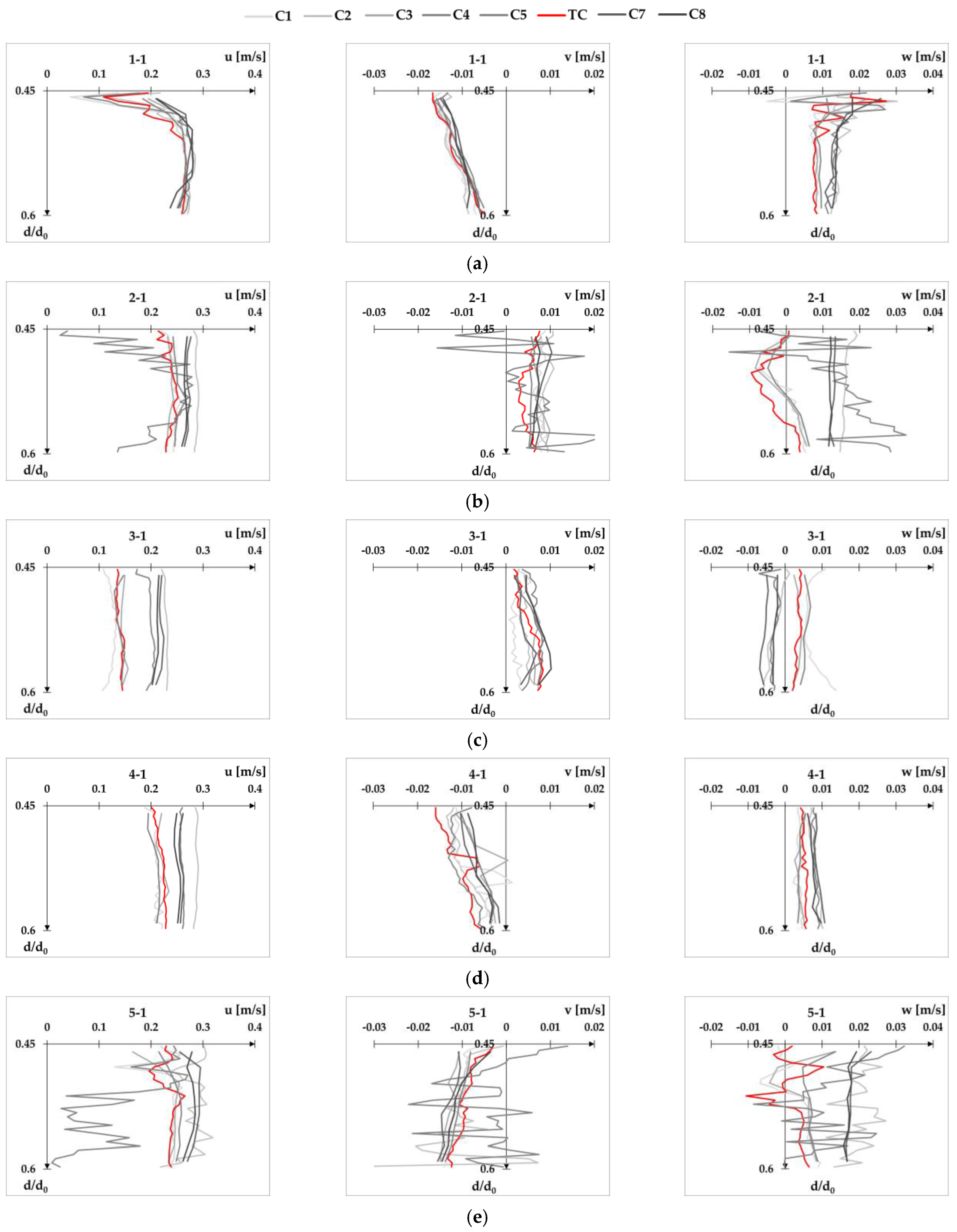
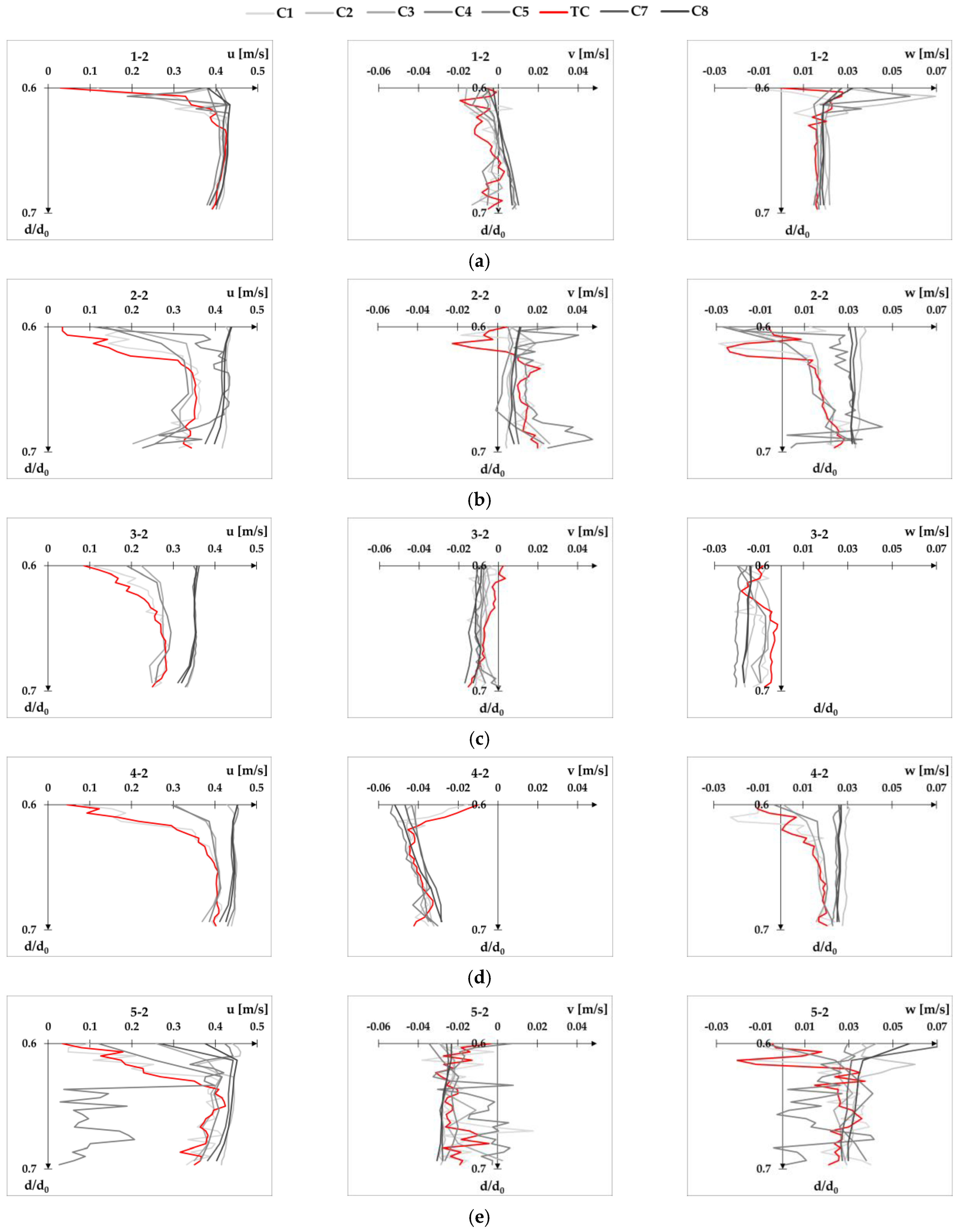
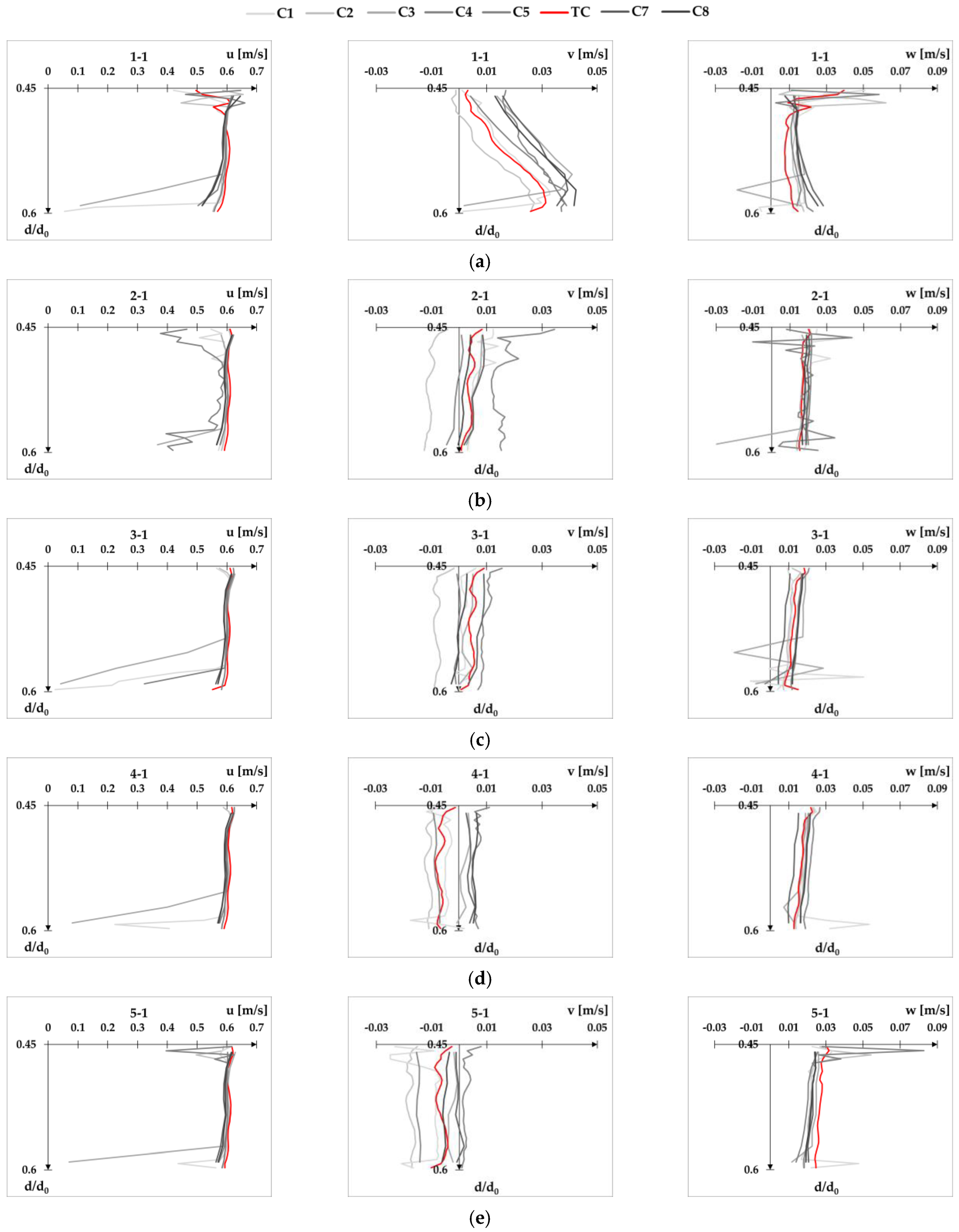
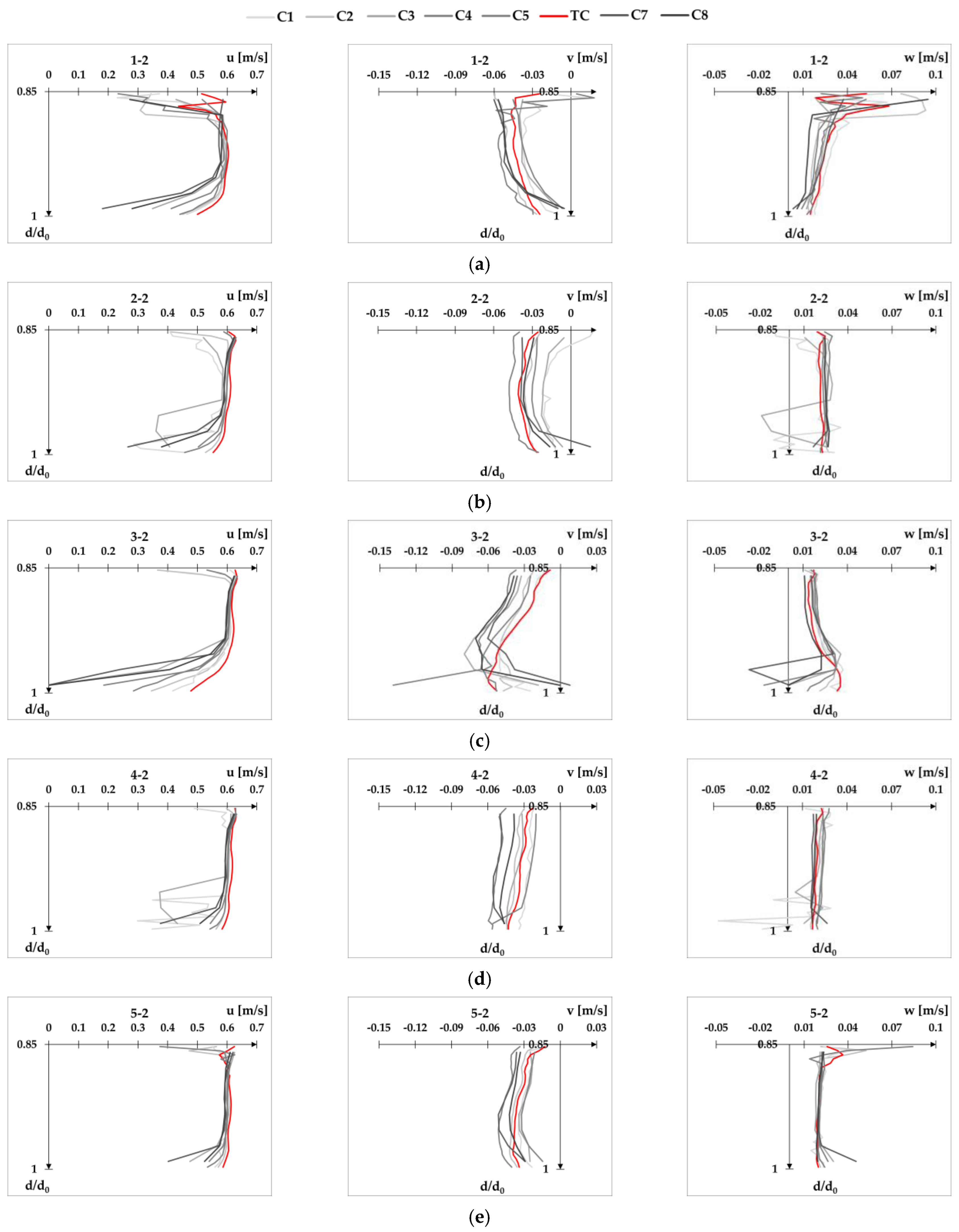
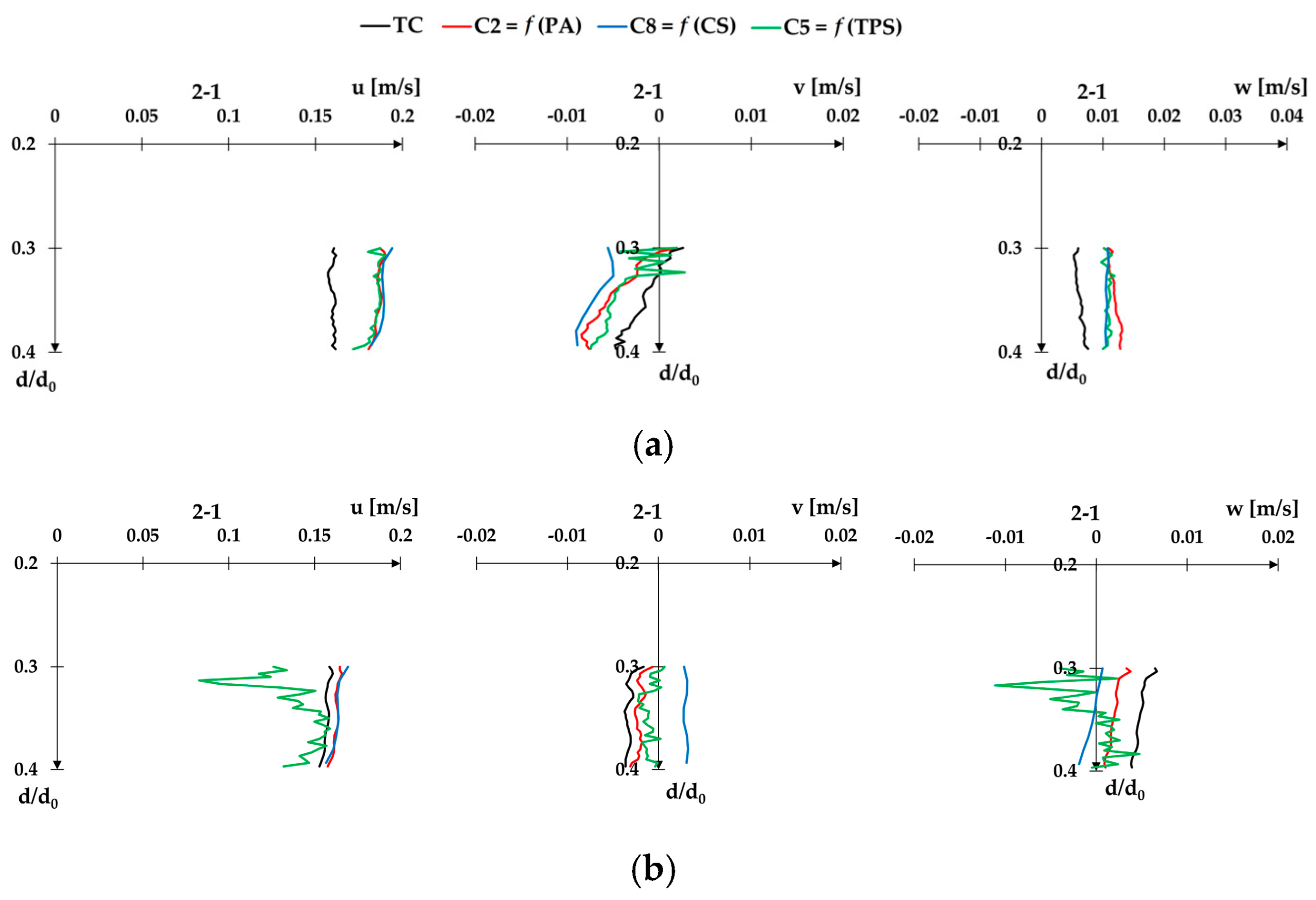
Configuration C5 provides the most scattered results for both cross-sections, resulting in the largest overall RMSE values. This can be seen in the following excerpt from Appendix A (Figure 9), which shows a characteristic vertical velocity profile for both cross-sections and all velocity components.

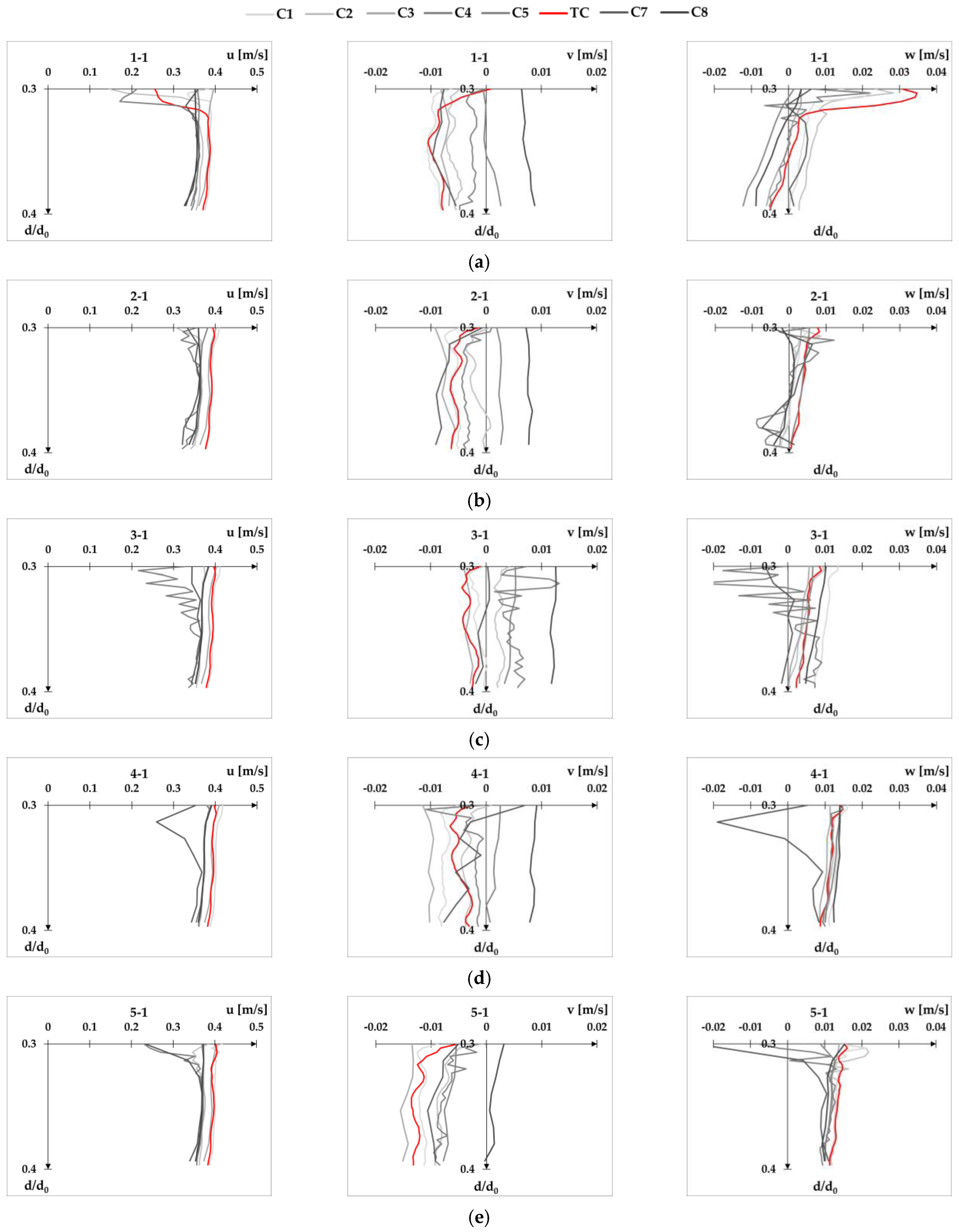
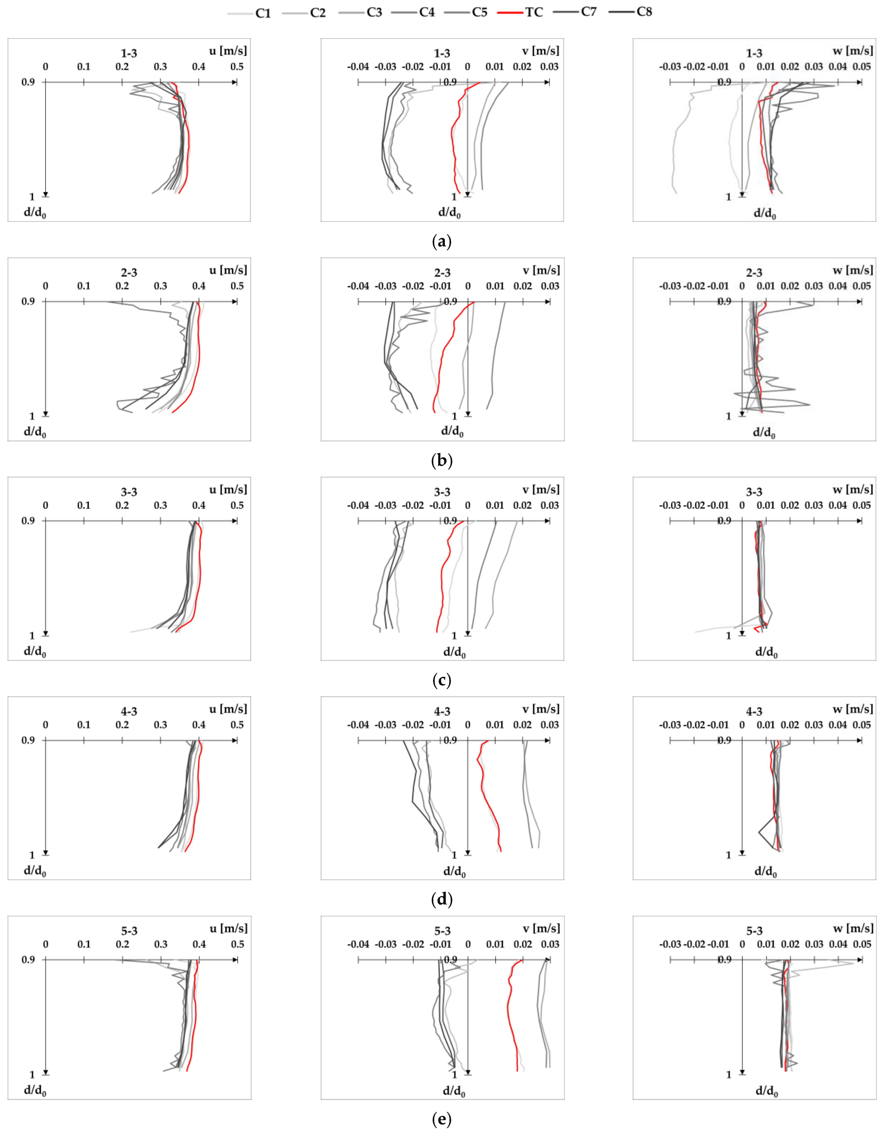
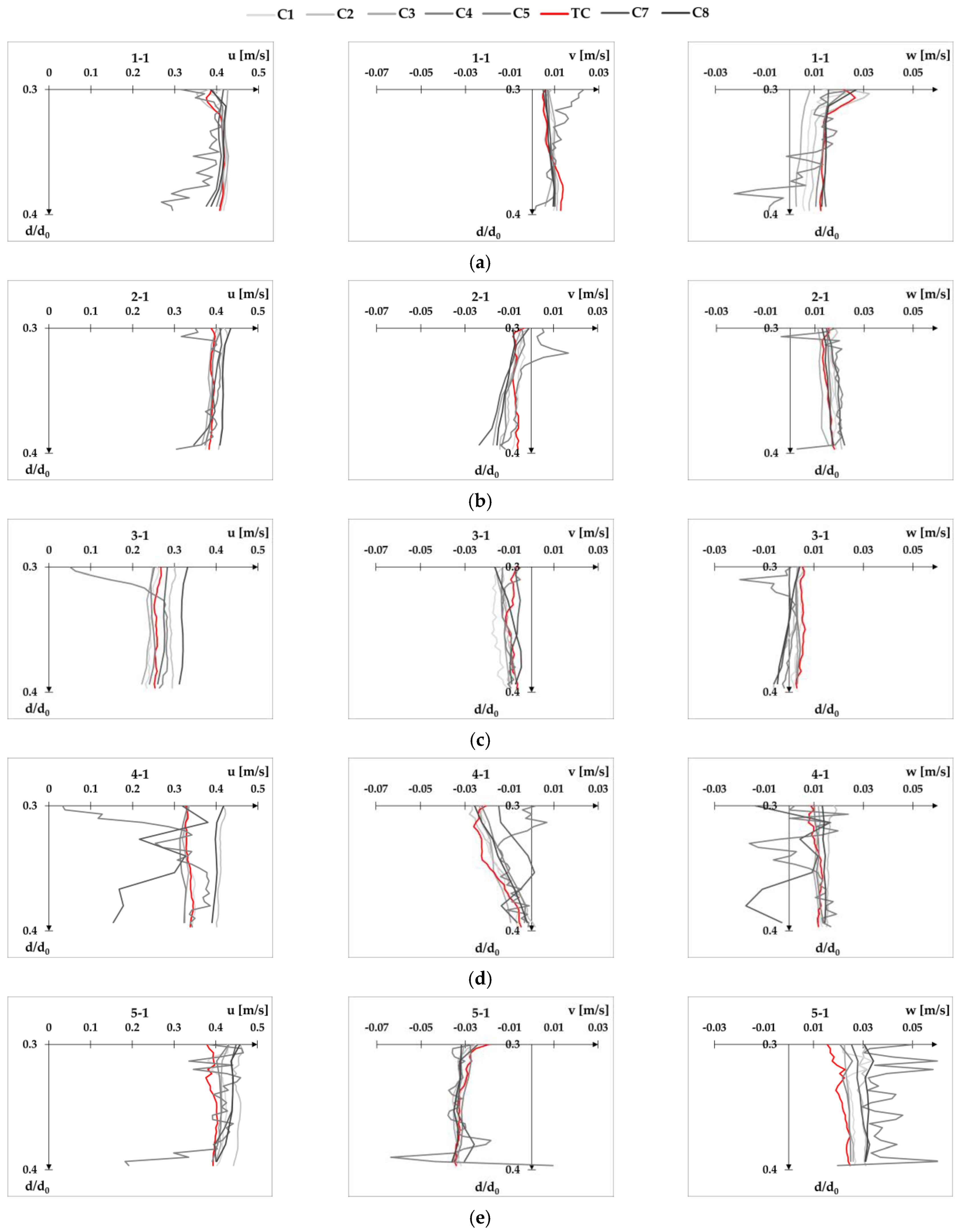
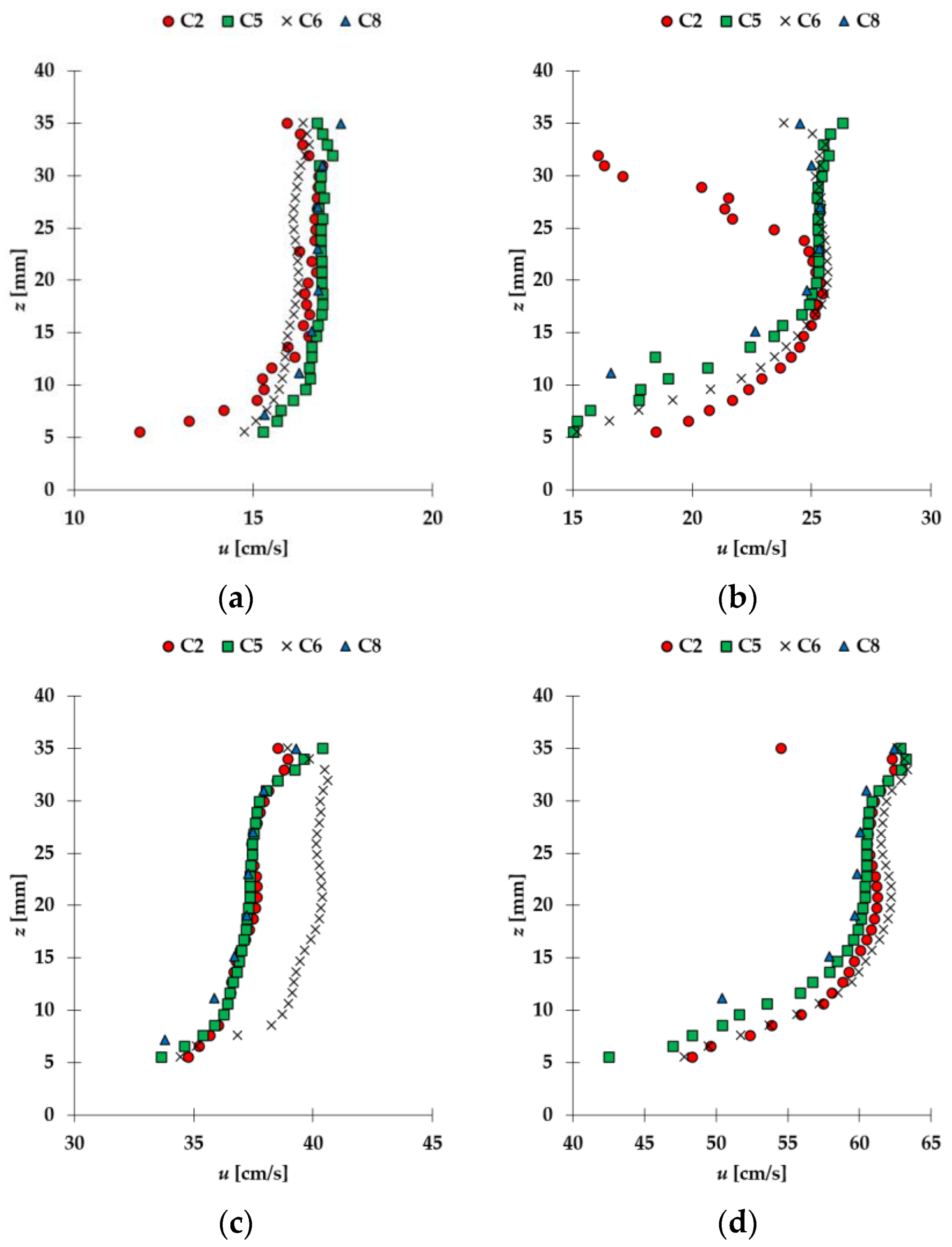
The velocity profiles for all eight configurations of the ADVP’s operational parameters are given as the appendices to this paper. For completing the velocity profiles, composite figure for velocity profile XS-US is presented as Appendix E. Figure A21 presents a comparison of detailed velocity profile in the near bed region for the flume mid-section for each probe configuration, consisting of four subplots (one for each flow condition). Velocity profile in this section follows log law, as reported by Pandey et al. [53] for similar flume setup. Appendices are structured to present each velocity component across the measurement points under both cross-sections. Appendix A contains velocity profiles for flow condition Q1d1, Appendix B velocity profiles for Q1d2, Appendix C velocity profiles for Q2d1, Appendix D velocity profiles for Q2d2, Appendix E velocity profiles for XS-US mid-section, and Appendix F contains profiles of cumulative average of TKE for Q1d1 and Q2d2.

4. Discussion

The values of the RMSE for the velocity component u show a strong dependence on the flow conditions: higher flow rate and lower flow depth (Figure 10 and Figure 11). On the other hand, the measured values of the velocity components v and w are also more sensitive to the higher flow rate than to the flow depth.

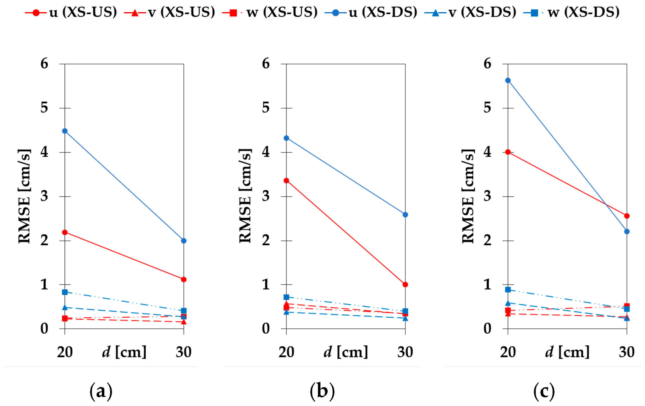
Changes in flow depth at a constant flow rate do not produce consistent results. Reducing the flow depth for the lower flow rate Q₁ leads to higher RMSE values in all velocity components for all three configurations (Figure 12). The RMSE values for all configurations give a high scatter for the higher flow rate Q₂ (Figure 13). RMSE values for the velocity component u are higher with increasing flow depth at XS-US under the configuration C2, while the RMSE values are lower with increasing flow depth under configuration C8 and become higher upstream and lower downstream under configuration C5 with increasing flow depth. For the velocity component v, the RMSE values under configurations C2 and C5 increase with increasing flow depth, while under configuration C8, they increase at XS-US and decrease at XS-DS. For the velocity component w, there is no significant change in RMSE with the change in flow depth.

The results show that each parameter change has a significant effect on the measured values of each velocity component when compared to TC. There is also an apparent trend where RMSE increases with the flow rate under the same flow depth. If the flow rate is constant at lower Q₁, an increase in flow depth reduces RMSE for both cross-sections and all velocity components. For larger flow rate Q₂, an increase in flow depth generally increases RMSE, but only for w, while the trend for u and v velocities varies. Differences in the RMSE values for the different ADVP parameters (Figure 5, Figure 6 and Figure 7) show that changing PA has the least effect on the velocity measurements while changing TPS has the greatest effect and causes the greatest errors in the data. The change in the PA from Adaptive to Max interval shows that there are fewer errors in the steady part of the flow but more in the turbulent flow.

Adaptive PA provided better overall results than the Max interval for the same CS and TPS, with also higher SNR and Correlation values, similar to the findings reported by Liu et al. [54] who state that Max interval PA always made the SNR and Correlation lower. If the velocimeter data are limited in their quality because of the seeding of the flow, the SNR and Correlation will be low. In that case, the PA may better be changed to Max interval, as shown in [54]. Our case was well seeded, so adaptive PA was sufficient to get the good quality data which also satisfied the visual check of velocity profiles (see Appendix A–D). In the study by Liu et al. [54], it is pointed out that the Max interval was the more appropriate PA based on visual evaluation of the velocity profiles, regardless of the lower SNC and Correlation values associated with the results. In the setup used for this paper, flow is disrupted by complex hydraulic structure (model pier and riprap), standard logarithmic velocity profile characteristic for the unobstructed flow is not expected, and velocity profiles are “random” which limits the applicability of visual evaluation of the velocity profile for XS-DS. However, the difference between Adaptive and Max interval PA is not significant, as demonstrated by Liu et al. (Table 3 from [54]), and as also stated in Part I of this research where differences between configurations C2 and TC are small for all metrics (see Table 3 from [29]). Liu et al. [54] also pointed out that CS and TPS should be treated with caution, which agrees well with the results of this study as discussed earlier, showing that TPS has the largest effect on the results, while CS has a larger effect than PA but not as large as TPS (Figure 5, Figure 6, Figure 7 and Figure 8).

The change in probe angle studied by Peltier et al. [55] resulted in smaller errors for the mean longitudinal velocity than the change in probe parameters. In the worst case scenario, changing the probe angle resulted in errors of up to 5% [55], while changing the parameters resulted in errors of up to 25% for the mean longitudinal velocity. The same trend can be seen comparing the change in sampling rate with the change in parameters. As Ruonan et al. [24] have shown, the change in sampling rate has a negligible effect on the time-averaged velocity, but it has a larger effect on the turbulent kinetic energy and the Reynolds stress, which can also be assumed for the change in parameters, as it already has a large effect on the time-averaged velocity.

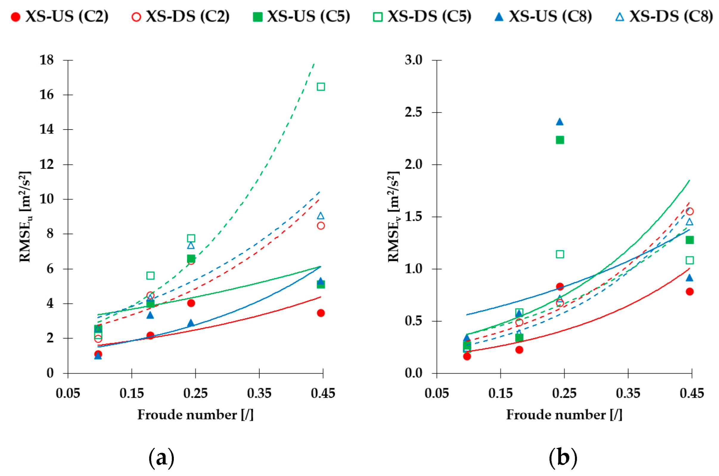
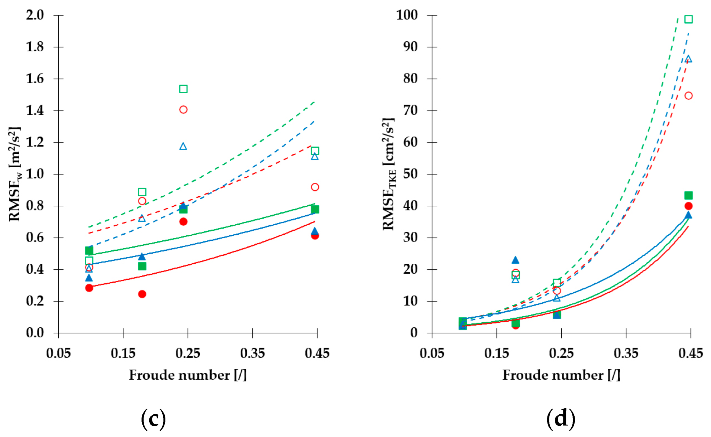
Since it is evident from both RMSE data and visual evaluation of velocity profiles that selection of ADVP’s operational parameters result with different error for XS-US and XS-DS, as well as for different flow conditions (Figure 5, Figure 6, Figure 7 and Figure 8, Table 2, Table 3 and Table 4), investigation was further expanded to evaluate dependence of the error as a function of dimensionless flow parameter, namely Froude number (Fr) used as reference for model scale. The following figure (Figure 14) shows change in RMSE for velocity components u (Figure 14a), v (Figure 14b), w (Figure 14c), and TKE (Figure 14d) as function of Fr. Since the flume has rectangular cross-section, Froude number increases with the mean flow velocity (V_Q1d1 < V_Q1d2 < V_Q2d1 < V_Q2d2) and its corresponding values are 0.10, 0.18, 0.24, and 0.45, respectively. General trend of error increase with larger Fr can be observed for all velocity components, as well as TKE and on both XS. For all three velocity components, it can be observed that flow condition Q2d1 (Fr = 0.24) RMSE deviates from trend, where RMSE is peaking for v and w velocity component on both XS and all configurations. For all three velocity components, RMSE values are higher than for Q2d2 (Fr = 0.45), except for RMSE_u change in CS (configuration C8). Correlation with TKE exhibits consistent increase in RMSE with increase in Fr, and correlation is overall stronger than for any velocity component (

Table 5. Calculated R² for correlation between Fr and RMSE for AC configurations.

Cross-Section	AC Configuration	R2 (u)	R2 (v)	R2 (w)	R2 (TKE)
XS-US	C2	0.39	0.48	0.41	0.99
	C5	0.26	0.13	0.51	0.99
	C8	0.80	0.03	0.30	0.68
XS-DS	C2	0.79	0.99	0.13	0.97
	C5	0.96	0.48	0.24	0.99
	C8	0.78	0.97	0.50	0.97

).

When correlation is evaluated using the coefficient of determination (R²), it can be seen that error in TKE shows a strong correlation (R² > 0.68) with increase in Fr, while the R² with velocity components is lower. When correlation with velocity components is analyzed, only consistent trend that can be observed is that R² for u and v velocity components is always higher for XS-DS than for XS-US, for all configurations. This confirms previous discussion about velocity profiles where it was observed that velocity profiles influenced by the pier and riprap are too random to be evaluated through visual observation. R² values for correlation between the Froude number and RMSE for all velocity components and TKE are given in the table below (Table 5).

5. Conclusions

Reliable turbulence data during flume experiments can be collected only if data collection instruments are properly configured. Otherwise, the error introduced into measurement will inevitably be propagated further into the analysis. This paper presents the differences in flow velocity profiles measured with eight different configurations of ADVPs’ operation parameters through the sensitivity analysis quantified via RMSE. The optimal configuration against which all others were evaluated was configuration C6, defined as the most accurate for flow measurement around the bridge pier in Part I of this research that was configured according to the following parameters: PA set to Adaptive, TPS equal to 4 mm, and CS of 1 mm. Whereas in Part I of this research, the goal was to identify the optimal probe configuration for downstream measurement of the complex hydraulic structure (pier protected with riprap) based on a match of the flow rate with measurements from other instruments, in this paper, the effect of distinct probe configuration on velocity profile and TKE is demonstrated.

When velocities measured using the AC configurations are compared with TC, the largest RMSE is observed when TPS is changed, followed by CS and PA. Absolute RMSE calculated for TPS change from 4 mm to 1 mm is, on average, 6.30 cm/s, 0.90 cm/s, and 0.82 cm/s for velocity components u, v and w, respectively. Absolute RMSE calculated for CS change from 1 mm to 4 mm is, on average, 4.49 cm/s, 0.88 cm/s, and 0.71 cm/s for velocity components u, v and w, respectively. Absolute RMSE calculated for PA change from Adaptive to Max interval is, on average, 4.04 cm/s, 0.63 cm/s, and 0.68 cm/s for velocity components u, v and w, respectively. For a change in all parameters, RMSE is greater for XS-DS than XS-US: on average, 90%, 57% and 54% for a change in PA, TPS, and CS, respectively. This is to be expected since XS-DS is positioned in a turbulent flow downstream of the bridge pier, which may cause a higher sensitivity of the ADVP, while XS-US is positioned in the approach section of the flow. In general, it can be expected that error increases with increase in flow severity, as shown through correlation with Froude number.

RMSE increase is also observed when the flow rate increases from Q₁ to Q₂ while retaining the same flow depth. RMSE increase at both cross-sections is similar for a change in PA. For flow depth d₁, RMSE is increased on average at 256% and 218% for XS-US and XS-DS, respectively, and 83% and 89% for flow depth d₂ at XS-US and XS-DS, respectively. For a change in CS, RMSE is increased on average by 187% and 260% for XS-US and XS-DS, respectively, and 50% and 164% for flow depth d₂ at XS-US and XS-DS, respectively. For a change in TPS, RMSE is increased on average by 262% and 186% for XS-US and XS-DS, respectively, and 56% and 114% for flow depth d₂ at XS-US and XS-DS, respectively. There is also an apparent trend where RMSE increases with the flow rate under the same flow depth. For the lower flow rate, as the flow depth increases, the RMSE value decreases for both cross-sections and all velocity components. However, for the higher flow rate, the RMSE value generally increases with increasing flow depth, except for the varying trend for u and v velocities. RMSE trend of TKE resembles the one of the velocity components in a way that general increase in RMSE with increased mean flow velocity is present. However, the value and differences of RMSE below the largest flow velocity (Q2d2) are not significant. Similarity of TKE with velocity is evident through RMSE increasing for configurations from C2 to C5, confirming that measurements are most sensitive to change in TPS, and least sensitive to change in PA.

Differences in the RMSE values for the different ADVP operation parameters show that changing PA has the least effect on both the velocity and TKE measurements while changing TPS has the greatest effect on them and causes the greatest errors in the data. Additionally, detailed velocity profiles show that changes in parameters can also distort the entire velocity profile. Therefore, the selection of optimal ADVP operational parameters should be considered and tested for desired application to ensure maximum data quality.