Article

Investigation of Recirculating Marangoni Flow in Three-Dimensional Geometry of Aqueous Micro-Foams

Department of Mechanical and Product Design Engineering, Swinburne University of Technology, John St., Hawthorn, VIC 3122, Australia
*
Author to whom correspondence should be addressed.
Fluids 2023, 8(4), 113; https://doi.org/10.3390/fluids8040113
Submission received: 14 February 2023 / Revised: 7 March 2023 / Accepted: 21 March 2023 / Published: 28 March 2023

Abstract

:
Experimental investigations of Marangoni flow in micro-foams have faced challenges due to the inherent difficulties in detecting and measuring this flow. The Marangoni flow manifests as small spots within the lamellae films, which makes it hard to accurately analyze. Hence, to elucidate Marangoni flow characteristics, this study introduces and investigates comprehensive three-dimensional models of flow in microscale foams. The geometric models contained Plateau Borders (PB), nodes, and films. The recirculating Marangoni flow was simulated and studied for different interfacial mobilities. Inside the foams, the Marangoni flow velocities were at the same scale with the PB flow velocity for mobile interfaces. However, for a more rigid interface, the magnitude of the Marangoni flow was considerably less than that of the PB owing to the combined effect of high surface hydraulic resistance on the Marangoni flows and nature of the Marangoni flow as a surface-only flow type. Furthermore, the effect of the film thickness on the Marangoni flow was analyzed. Thicker films have a stronger effect in reducing the Marangoni flow than PB flow. This is due to the higher ratio of gravity body force to the Marangoni-driven surface force for thicker films. Finally, the combined effect of the liquid–air interfacial mobility and film thickness on the Marangoni velocity was studied.

Graphical Abstract

1. Introduction

Aqueous foams have attracted the attention of several scientists and researchers. They are widely used in different industries, such as cosmetics, oil recovery, and natural gas deliquification [1,2,3,4]. They are equally useful in washing basins, spraying crop (agriculture), dampening explosions, removing radioactive dust, and collecting proteins in the food industry and desirable elements in the mineral industry [1,2].
Aqueous foams comprise gas and a limited liquid volume fraction, which are categorized into two types: wet and dry aqueous foams. Wet foams have a volume fraction of 10–20% liquid and bubbles with spherical shapes, while dry foams have less than 5% liquid [5], and their bubbles have a polyhedral-like shape. The faces of the polyhedral bubbles are called lamellae and comprise thin liquid films. The conjunction of these lamellae films makes a channel known as the Plateau Border (PB), while those of the four PBs make a node [6,7].
Several factors can affect the dynamics and behavior of the foam and flow inside the foams, respectively, such as the drainage, surfactant materials, surfactant concentration, and Marangoni effect [8,9,10]. The Marangoni effect is named after Carlo Giuseppe Matteo Marangoni, who discovered this phenomenon when writing his doctorate thesis in 1865 [11]. The main factor in this phenomenon is the existence of surface surfactant concentration gradients [12]. Surfactants are water-soluble chemical components [13,14]. The complex shape of the surfactants is key to creating surface tension. The surfactants have hydrophilic heads and hydrophobic tails located at the free surface, which effectively decrease the surface tension [15]. Surface tension gradients and Marangoni flows in aqueous foams can occur in different processes and systems, such as foam fractionation [16,17,18,19], UV photo-surfactants [20], and foam recirculation [5,21]. Foam fractionation uses the rising columns of foam to remove hydrophobic molecules from liquid solutions [16]. This process is also known as protein skimming; it is used in industries to remove surface-active contaminants from wastewater. Robert Lemlich characterized a model for foam fractionation in 1960 and demonstrated how foam fractionation columns could be operated in the presence of external refluxes which induced the Marangoni flow [17,18,19].
Exposing photo-surfactants to ultraviolet (UV) light is another method that can cause the Marangoni flow. Chevallier et al. [20] studied this phenomenon and the effects of UV rays and photo-surfactants’ concentration on the drainage flow in thin aqueous films as well as real-size foam in containers. They discovered that UV rays caused a difference in surface tension in the films and PB, thereby inducing the Marangoni flow.
Surface surfactant concentration gradient, which is caused by the influence of PB branching in the nodes, is another system method that causes the Marangoni flow. When bulk flow branches to three PBs, each surface flow branches to two surfaces. Hence, the entering bulk liquid with the flow rate of q and surface surfactant of Γ e q will have three q/3 flow rates and six surfaces surfactant of 2 / 3 Γ e q . This branching changes the bulk and surface flow balance and creates a surface tension gradient between two nodes, thereby causing a Marangoni flow. This system was introduced by Pitois et al. [21], who demonstrated that the hydrodynamic resistance and permeability of PBs depended on the dimensionless Boussinesq number (Bo) and upward velocity of the Marangoni flow. They investigated the Marangoni effect in the transitional regions for conventional Tetradecyl Trimethyl Ammonium Bromide (TTAB) with a constant Gibbs elasticity of 0.01 N / m [21]. Gibbs elasticity for different surfactants was studied in detail by Mondy and Lucassen [22,23].
It is noteworthy that despite the significant experimental [5,21] and theoretical research [7] on the Marangoni flow, limitations in this area still exist. As regards experimental studies, the limitations are primarily owing to measurement problems. Pitois et al. [21] reported in their study, “We were not able to measure the liquid velocities over such small lengths. Instead, we followed the upward motions of surface irregularities (thin spots) in the films near the channel/film transition region”. In theoretical studies, these limitations were owing to the lack of a precise three-dimensional model that captured the flow characteristics of nodes, PBs, and films. Anazadehsayed et al. [7] modeled a system containing a PB and node to investigate the effect of Bo on the flow in the PB’s interior and exterior foams (the exterior foams are the external part of the foam where the bubbles connect to the container wall, while with the interior foams, the bubbles are inside the net).
Using their groundbreaking research, we have developed a novel three-dimensional geometry and model that includes a PB, node, film, and transition region for our study. This advanced three-dimensional configuration has allowed us to investigate the effects of branching on surface flow, which is closely linked to bulk flow (as introduced by Pitois, Figure 1 of recirculation model for liquid flow in foam channels [21]). Our model also takes into account the crucial role of nodes, as previous research has shown that the velocity of bulk flow decreases significantly after being trapped by a node [24,25,26]. Therefore, using a 2D system or neglecting the presence of nodes would significantly impact our results. Furthermore, we validated our model using previous experimental and analytical studies [8,21,27]. We investigated the influence of interfacial mobility (different Bo numbers) on the Marangoni flow. The flow behavior in the exterior film and PB was compared to that in the interior film for different Bo numbers. Finally, a master curve was developed for Marangoni flow velocities for dimensionless interfacial mobility and film thickness.

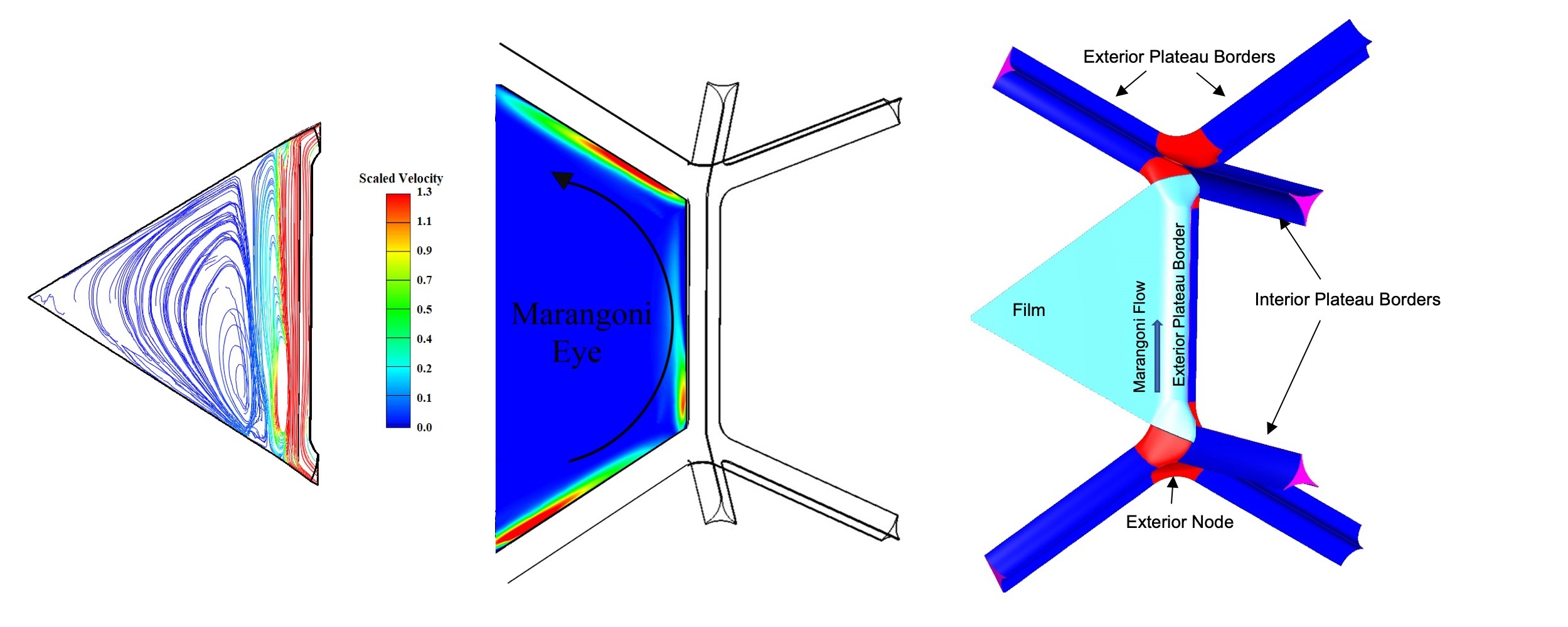
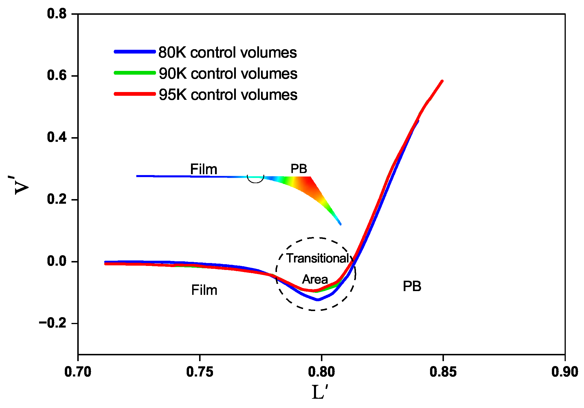
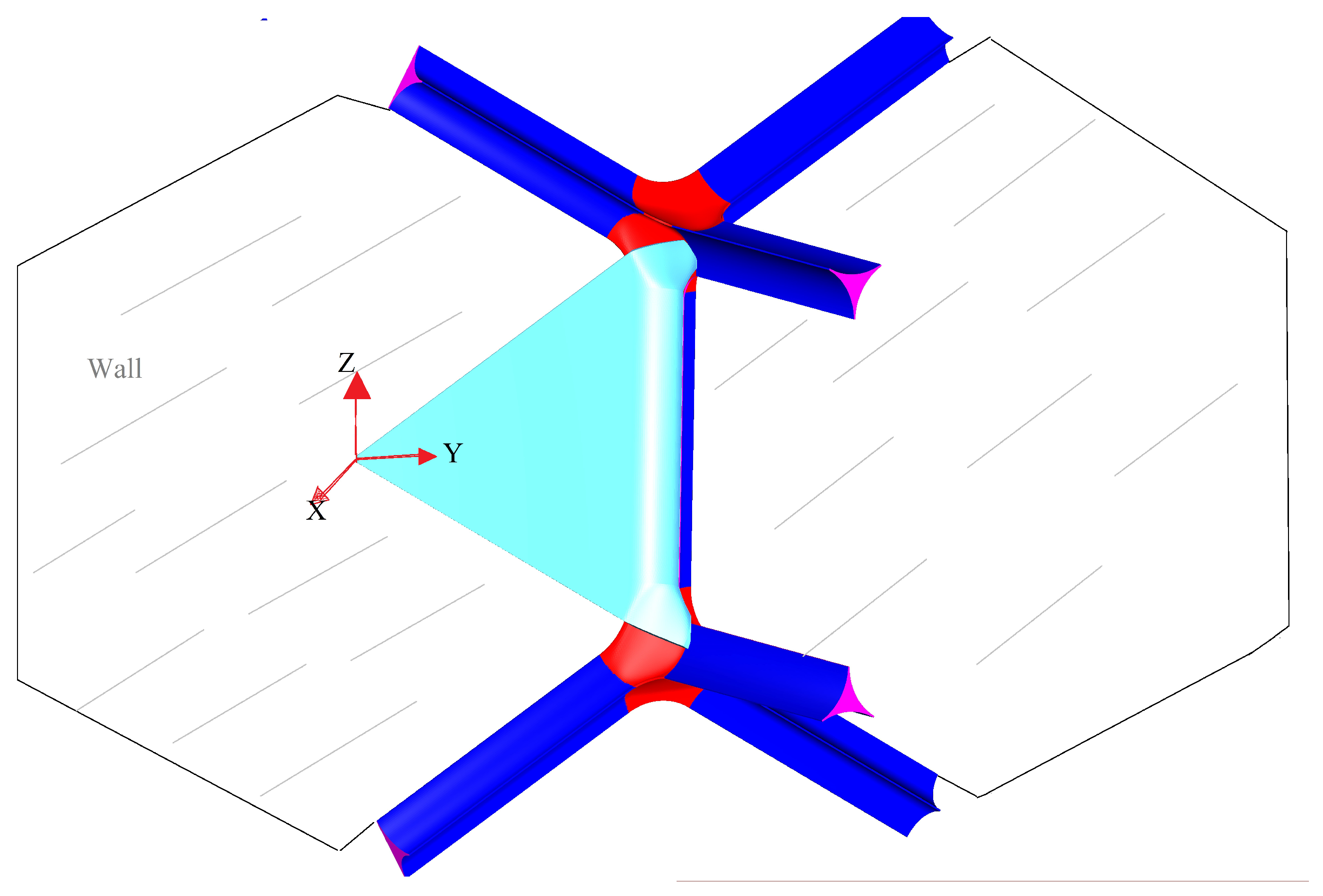
2. Geometrical Model

In this study, both the interior and exterior foams were considered for studying the Marangoni flow behavior. Interior foams are formed in the interstitial region between the three neighboring bubbles, while exterior foams are formed in the region between the two neighboring bubbles and a rigid container wall. However, the interior foams were not connected to any container wall. The conjunction with the exterior wall led to a change in the geometry for the PBs, films, and nodes. This change in the exterior geometry led to a distinct difference between the flow behaviors in the interior and exterior foam models, owing to their different boundary conditions, such as the zero-velocity boundary condition (the zero-velocity area is at the intersection of the PB and film with the container wall).
The exterior nodes were constructed together with three exterior PBs with an angle of 120 , wherein two PBs were attached to the wall and one was perpendicular to the wall. Note that the interior and exterior PBs have a similar transverse radius of curvature R. The film thickness ( α ) for exterior geometry is the distance from the wall and conjunction of PB to the film, while for interior geometries, this distance is the interior film thickness. The details of the geometry measurements and simulation parameters are presented in Table 1.
In this study, both the interior and exterior geometries of the foam network were constructed in three dimensions. Each of them comprised Plateau Borders, nodes, and films. The geometry of the interior foam is shown in Figure 1a; The six-fold symmetrical area (colored in sky blue) contained 1/6 of the inlet, outlet, nodes, PB, and film (for more information about the mesh and its specific details, please refer to Figure A1). The flow entered from the top of the three PB inlets and exited from the three interior outlets at the bottom. The geometry of the exterior foam is shown in Figure 1. The governing equations were solved for the geometry as shown in Figure 1a,b.
In Figure 1b, the flow enters from the top of the three PB inlets and exits from the other two exterior PBs and a single interior PB. It is noteworthy that the bubbles that formed the foam network were assumed in a tetrakaidecahedral shape, and the foam was considered to be a dry foam with a low liquid volume fraction, ε 0.05 , wherein the channels were long and slender [5] (radius of curvature of the PB and PB length are listed in Table 1).
For the current exterior geometries (Figure 1b), the symmetry boundary condition on the cut surface of the geometry and zero-velocity boundary condition was used in conjunction with the vessel walls. It is noteworthy that the container wall was assumed to be a nonslip (solid) wall to which the current exterior node–PB film system was attached. In Figure 1b (and for better clarification, please refer to Figure A2), the exterior inlets/outlets, nodes, and PBs were attached to the container wall.

3. Governing Equations

In this study, the numerical simulations were performed using AVLfire 2017 and 2020, which is a commercial software that is widely used for simulating complex fluid dynamics phenomena. The governing equations, which are based on the steady three-dimensional Navier–Stokes equations, were discretized using the Eulerian frame of reference cell-centered finite volume approach. The finite volume method is a numerical technique for solving partial differential equations that involves discretizing the domain into small control volumes, calculating the fluxes at the boundaries of each control volume, and then using these fluxes to update the solution values inside each control volume. The cell-centered approach used in this study means that the solution values are located at the center of each control volume, which is a common approach in fluid dynamics simulations. The SIMPLE (Semi-Implicit Method for Pressure-Linked Equations) method was used to couple the velocity and pressure fields in the Navier–Stokes equations. This method is a popular algorithm for solving the pressure–velocity coupling problem in incompressible fluid flow simulations, and it is known for its stability and robustness. It is worth noting that the Marangoni flow in microscale foams is typically laminar and steady, making the Eulerian approach with finite volume method a suitable option for simulating these flows. The assumption of incompressible fluid flow is also appropriate for the simulation of microscale foams, as compressibility effects are insignificant at these scales. The conservation of mass, momentum, and surface surfactant concentration were controlled by the corresponding equations.
Mass conservation:
· U = 0
Momentum conservation:
ρ ( U · ) U μ 2 U = p + ρ g
Passive scalar surface surfactant conservation:
s · ( Γ u s ) = 0
U and μ are the velocity (velocity vector) of the fluid and bulk viscosity, respectively. In the second equation, ρ ( U · ) U represents the convection and μ 2 U shear stress. The p represents the pressure gradient and ρ g (the buoyancy term) represents the gravitational body force. In the simulation, the second-order accuracy of the central differencing scheme was used for the momentum and mass conservations.
Equation (3) is the conservation law of surface surfactant concentration ( Γ ), where u s represents the velocity in the surface [29,30,31,32]. The comprehensive format of the conservation law of the surfactant mass is Γ t + s · ( Γ u s ) = S [29,30]. However, in this study, the S term containing the adsorption, desorption, and diffusion of surfactants were omitted for the simplicity of our model, which enabled us to particularly focus on the Marangoni flow. In Equation (3), Γ t (where t refers to time) was removed because of the steady state of the model, which is discussed in the next section. Further, due to the definition of Γ , which is only defined in the surface, the gradient operator was the surface gradient operator.

Boundary Conditions

In addition to the six-fold symmetries for interior and exterior geometries and applied static pressure in the inlet and outlet of the geometries (which are located at the top and bottom), the following boundary conditions were used:
Liquid–air interface of PBs and nodes
μ s 2 u s s 2 μ U n = 0
Equation (4) is based on the Leonard and Durand methods [33,34] while using Newtonian surface viscosity and small Reynolds number assumption. μ and μ s are the bulk and surface viscosities, respectively. n and s are the normal and tangential coordinate of the air–liquid interface, respectively. u s denotes the surface velocity in the tangential direction.
Equation (4) represents the decoupling of the surface and bulk layers. Decoupling is best described using the Boussinesq number ( B o ), which is a dimensionless value that shows the surface mobility. B o is proportional to the ratio of surface viscosity ( μ s ) to the bulk viscosity ( μ ) and is defined as B o = μ s μ R , where R is the radius of curvature of the channel and is assumed to be 100 μ m . Hence, B o is critical in the behavior of the flow on the liquid–air interface. In this study, B o numbers with the highest values (∼10 4 ) are considered as rigid walls, while B o numbers with low values (∼10 4 ) are considered as slip walls.
Liquid–air interface of the films:
μ s 2 u s s 2 μ U n γ Γ s Γ = 0
Equation (5) is the advanced version of Equation (4), which contains the surface surfactant concentration gradient [5,19]. The third term, τ = μ u s n = γ Γ s Γ , defines the Marangoni stress. s Γ is the tangential surface surfactant concentration gradient and γ Γ is related to Gibbs elasticity [14,34].
In this study, Equation (5) was applied to the surface of the film, where the direction of the Marangoni velocity was assumed in the z-axis of the Cartesian coordinates and in the opposite direction of the gravity force. However, Equation (4) was applied to the liquid–air interface of the PBs because the Marangoni flow was experimentally detected on the surface of the film [21] close to the conjunction of the PB and film (known as the transitional area).
Based on the methodology of Pitois et al. [21], the surface surfactant concentration or Γ change along the transitional area, and the associated surface tension gradient created a Marangoni flow from a higher Γ (or lower surface tension) to a lower Γ (or higher surface tension) [21,35,36]. This gradient can be attributed to the branching of a PB into three PBs in the node. Thus, Pitois et al. [21] introduced the q s u p as an upper surface flow rate, which was on the surface of the PB and moved toward the lower node, and q s d o w n as a lower surface flow that passed through the lower node and flowed on the surface of a new branch of the previous PB. Hence, as Pitois explained, q s u p had a higher rate than the downstream surface flow rate:
q s u p R u Γ e q
q s d o w n R ( 2 u / 3 ) Γ e q
where u, Γ e q , and R are the surface velocity of the PB, surface concentration of the surfactant further from node, and radius of curvature of the channel, respectively. Hence, there was a constant readjustment of the surfactant concentration from the lower stream to the upper stream.
According to Pitois et al. [21], the surface surfactant concentration for the geometry’s upper and lower stream are: Γ = Γ e q 0.1 Γ e q and Γ + = Γ e q + 0.1 Γ e q [21], respectively. Here, the characteristic length of R, Gibbs elasticity, and Γ e q are assumed as 100 μ m, 0.01 N/m and 10 6 kg/m 2 (Table 1), respectively, [22,23].
In our method, the governing equations of this study together with the aforementioned boundary conditions were applied to the simulations for the steady-state geometry. This is because of our assumptions were based on Pitois’s work, where Γ + and Γ on the upper and lower nodes forced the Marangoni flow at the interface of the film. This Marangoni flow had a higher value (maximum Marangoni velocity) at the beginning of the simulations before the surfactant concentration reached the equilibrium value (owing to a higher surfactant concentration gradient). Furthermore, this study focused on investigating the maximum Marangoni velocity (not the lifetime of a foam nor the duration to reach the equilibrium point) in different mobilities with different geometries and thicknesses. It is noteworthy that in this study, all the parameters were scaled based on Table 2.

4. Results and Discussion

In this study, the influence of the interfacial mobility on the Marangoni flow behavior in foam was studied. Our new three-dimensional models demonstrates fewer limitations than the two-dimensional models, which covered the entire geometry, including the films, PBs and nodes Figure 1a,b. To validate the accuracy of our newly developed three-dimensional models, we first verified that our results were independent of the simulation setup, particularly the number of grids. Furthermore, we compared our model results to previous experimental and analytical results. Finally, we predicted the Marangoni behavior for a wide range of B o values (from slip to rigid interfaces) and film thicknesses for both interior and exterior foams.

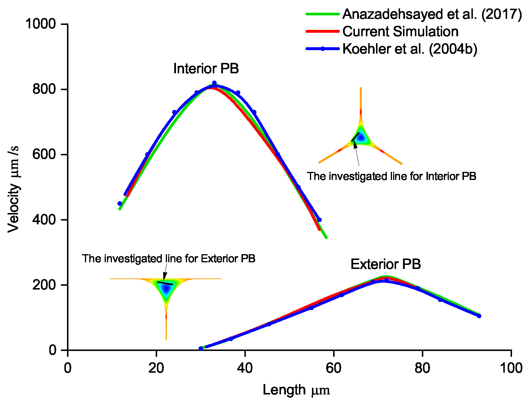
4.1. Models Validation

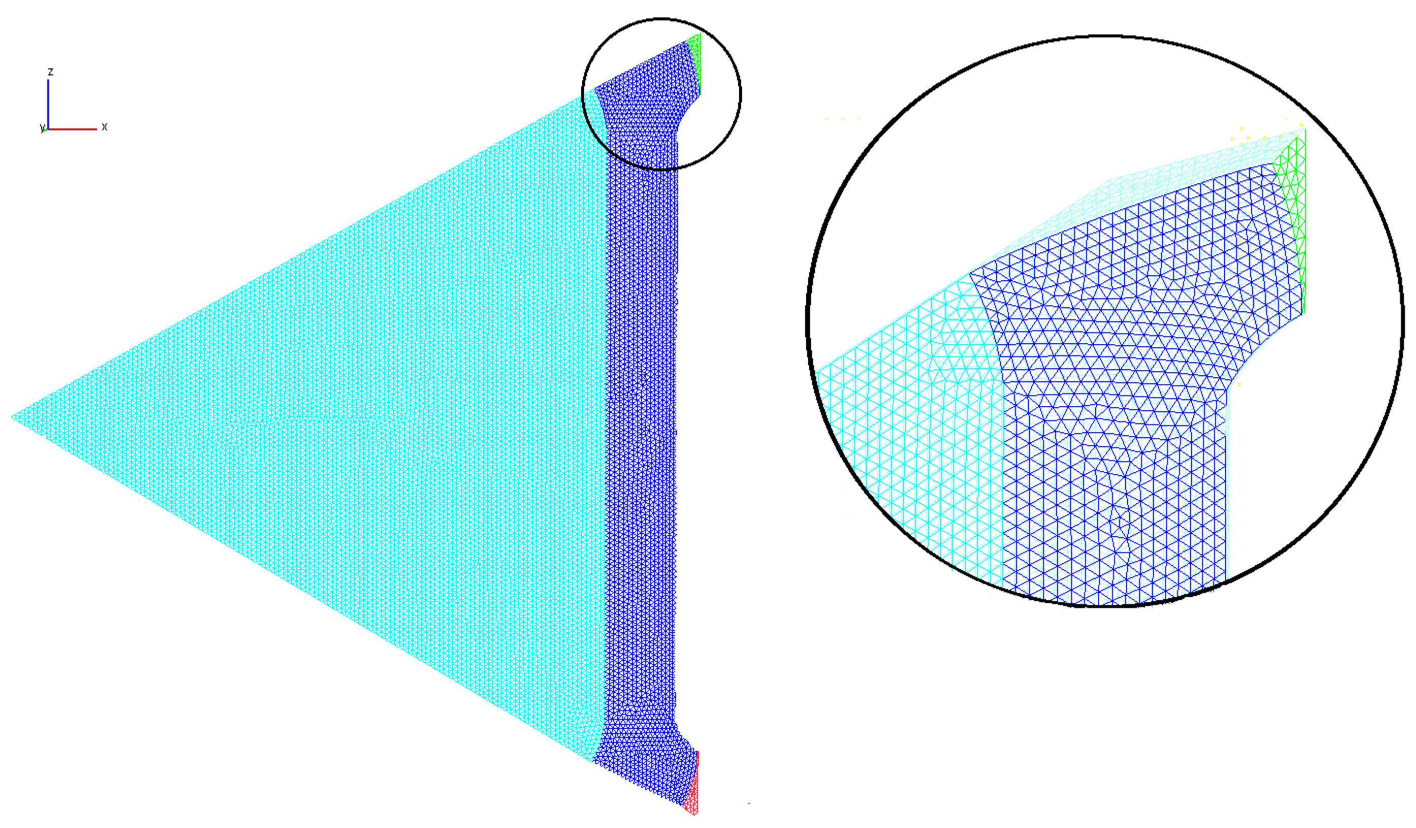
4.1.1. Grid Independency

Grid independency is important for any finite volume approach model to eliminate the influence of the grid cell sizes on the computational results. Figure 2 depicts the velocity profiles of the PB, transitional region, and film for different cell sizes, which are related to 80 k, 90 k and 95 k cells of a fixed volume. The velocity profiles were sketched along the length of the geometry from the edge of the PB to the center of the film (as shown in a cross-section of the geometry Figure 2) for sodium dodecyl sulfate (SDS) material. As shown in Figure 2, the profiles did not change considerably after 90 k cells. Hence, for all the simulations in this study, the geometries with cell sizes related to 90 k cells were used.

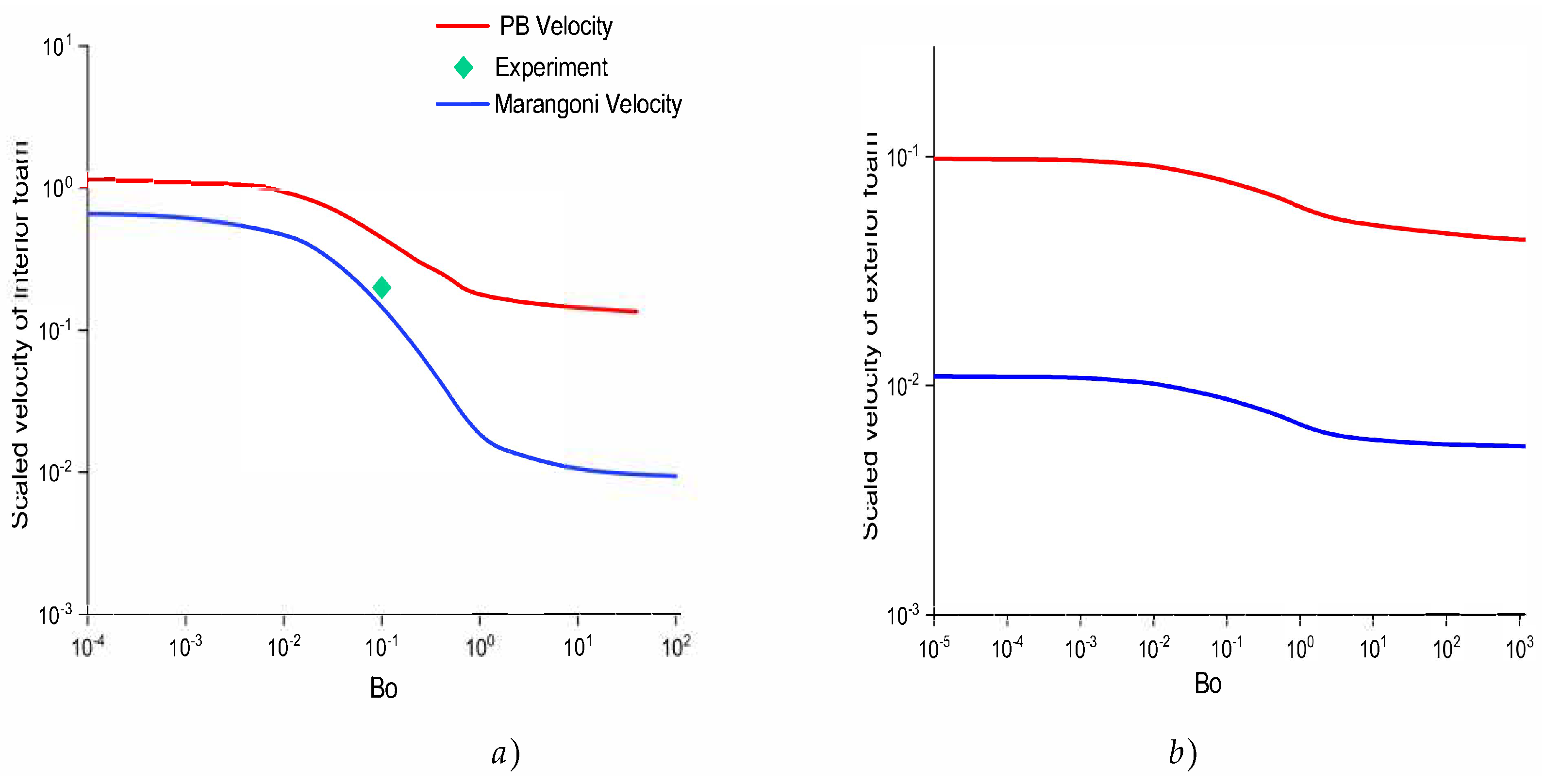
4.1.2. Experimental Validations

The results of this study were validated against the experimental data of Pitois et al. [21], who measured the Marangoni velocity in a film. In their experiment, they used 3 g/L concentration of TTAB in pure water. The results of the experimental data were compared to our simulated model as shown in Figure 3. The Marangoni flow in the film was sketched against the average liquid velocity in PB. The experimental data and current simulation showed consistency.
We also compared the flow in the PBs and nodes of our models using the experimental studies performed by Koehler et al. [37,38] and validation performed by [27]. Figure 4 shows the velocity of the flow inside the PB for the SDS foam. Our models and their experimental results for both the interior and exterior foams were consistent.

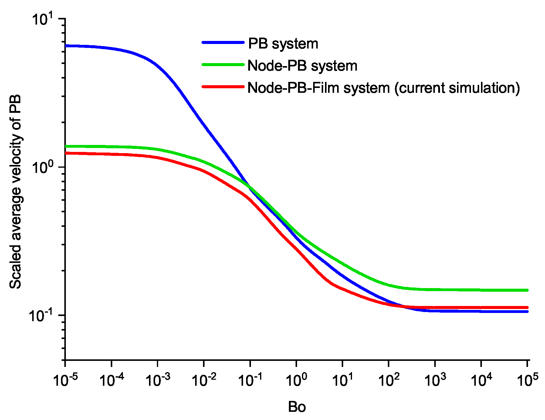
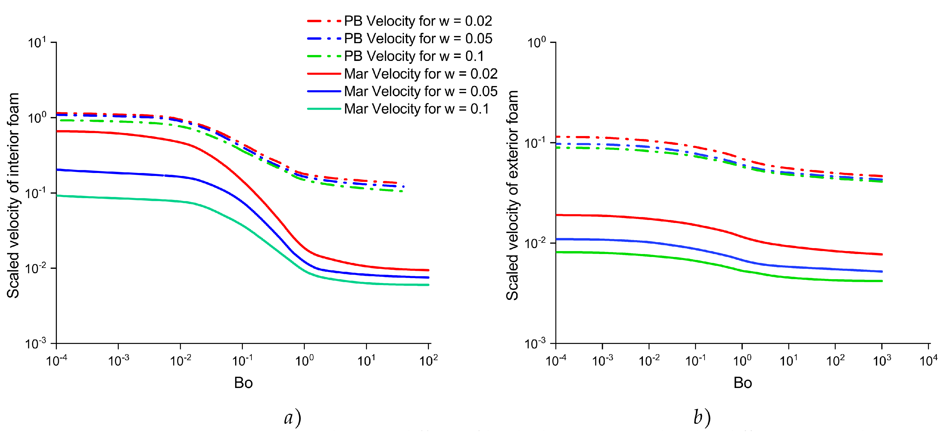
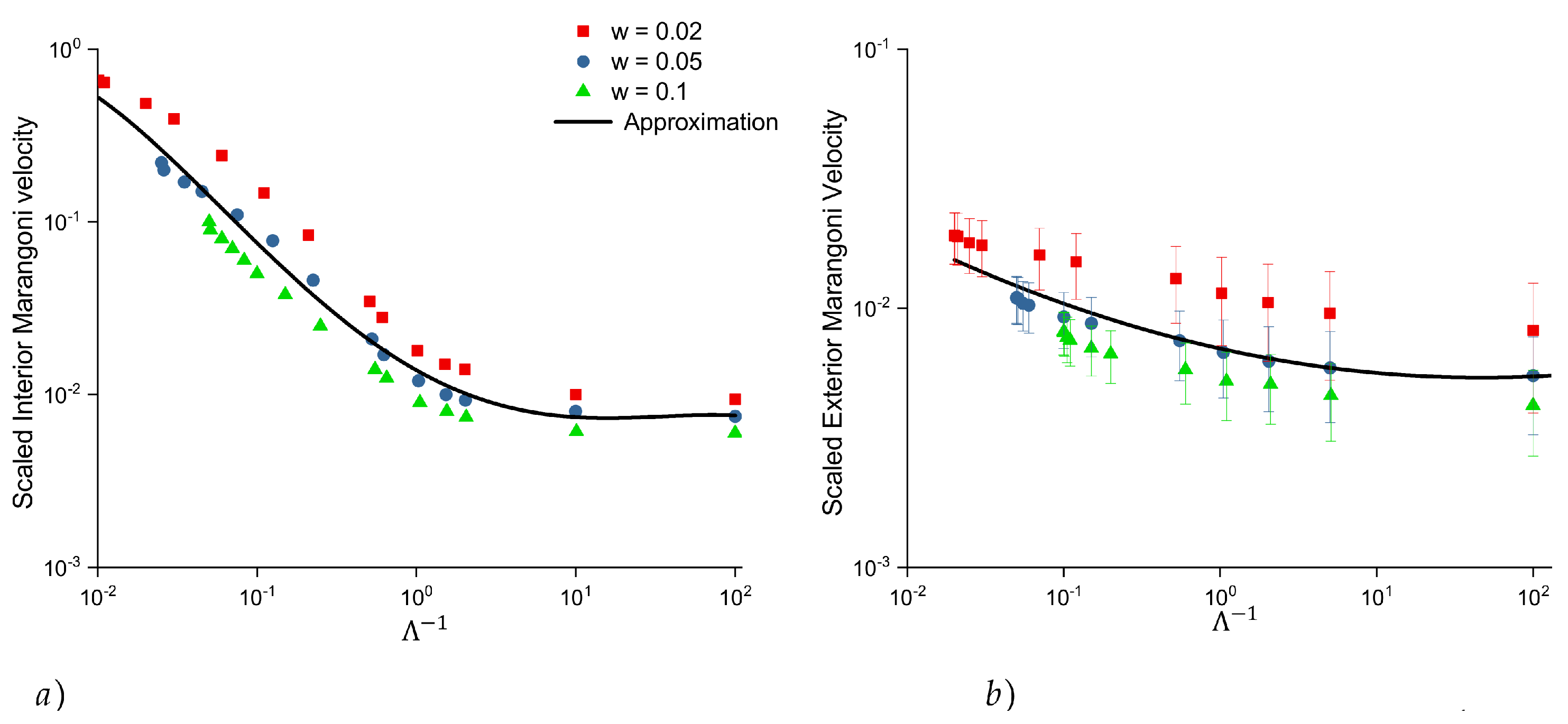
4.1.3. Analytical Validations

For the further validation of our models, we compared the velocity ranges of the node PB of our model to those in studies by Anazadehsayed et al. [27] and Nguyen et al. [8]. Anazadehsayed et al.’s [27] analytical results were based on a node–PB system; Nguyen et al.’s [8] results were based on a single PB system, and our results are based on an entire system containing nodes, PB, and a film. The three velocity ranges scaled by ρ g A μ (Table 2) are shown in Figure 5. The results of our study were similar to those of Anazadehsayed et al. [27]. However, they were different from those of Nguyen et al. [8] for lower Bo values ( 10 5 to 10 2 ). This is owing to the inclusion of dissipation and resistance in each node [27]. Our results corresponded with those of Anazadehsayed et al. [27].
Generally, our validations indicate that our three-dimensional PB–node–film models accurately captured the flow in the interior and exterior PB, node, and film. Additionally, the validations showed that our models were reliable for investigating the accurate contribution of Marangoni flow in interior and exterior foams.

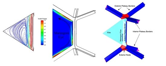
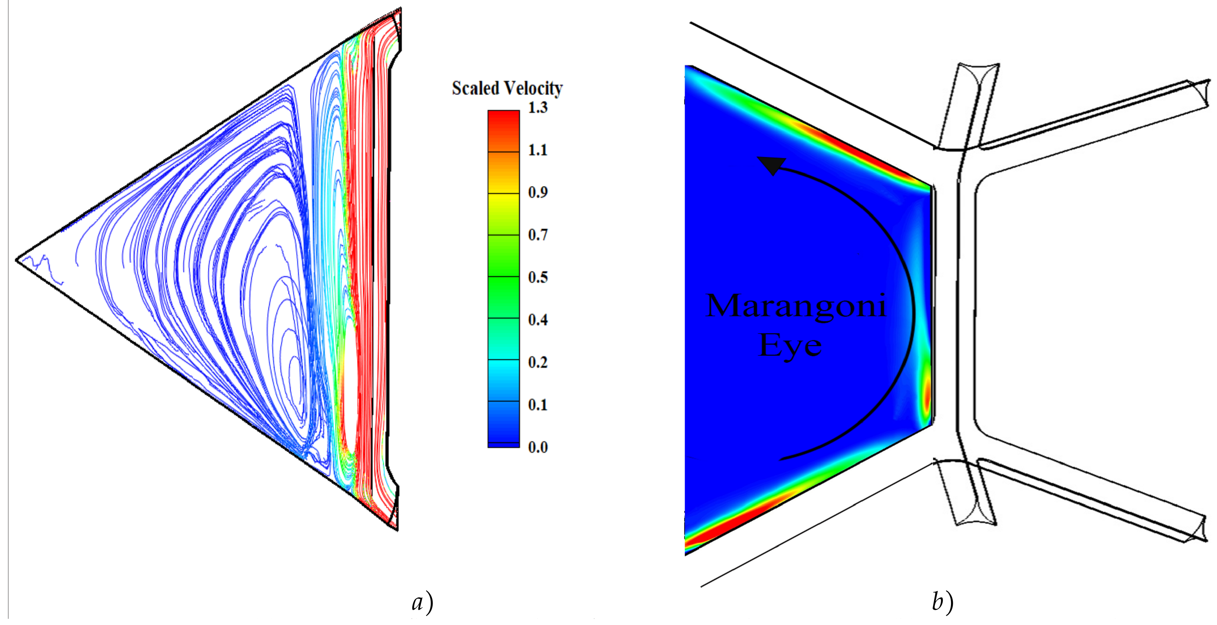
4.2. Recirculation Marangoni Flow

As mentioned above, detecting Marangoni spots in micro-foams is difficult. Hence, only a few experiments have been conducted to study this flow for different surfactants. This is even more complicated in exterior foams, where solid walls decrease the Marangoni velocity values considerably, thereby making the measurements more difficult. To solve this experimental limitation, this study developed models based on experimental and analytical validations. Marangoni flows were calculated in the transitional region. In Figure 6, the Marangoni flow for half of the film of an interior foam with R = 100 μ m is illustrated. As shown in Figure 6a, the flow caused by the Marangoni stress created a circulation pattern in the film between the upper and lower nodes [35]. This phenomenon is known as the Marangoni eye phenomenon in the film [35], as sketched in Figure 6b by combining three different simulations with the boundary conditions in different directions.
Notably, the Marangoni flow spots in the film appeared stronger near the bottom of the PBs [21] where the surface surfactant gradient was at its highest value.
As expected, when the liquid–air interface mobility increased, low Bo numbers occurred, which is similar to the scaled velocity of the node–PB. This was similar to the Marangoni velocity. However, the behavior of the Marangoni flow was different for interior and exterior foams. Figure 7a,b show the velocity profiles of the node–PB and Marangoni flow for the interior and exterior foams. The mutual characteristics of the node–PB and Marangoni flow in both the interior and exterior foams is the increase in velocities with a B o number decrease (more mobile interfaces).
However, in the exterior foams, the velocity ratio (Marangoni velocity to PB velocity) was almost constant for both the rigid and mobile foams (Figure 7b), whereas in the interior foams, this ratio was noticeable in rigid foams but less noticeable in mobile foams. This is revealed by the gap between both curves shown in Figure 7a. The gap was large for high B o numbers and small for low B o numbers. This behavior can be explained using the concept of hydraulic resistance.
As mentioned above, the Marangoni flow is a surface flow that is extremely dependent on surface mobility. In the interior foam, for mobile liquid–air interfaces, the node–PB and Marangoni velocities had similar values, particularly because both flows experienced a very low hydraulic resistance. However, in the same interior foam with rigid liquid–air interfaces, the surface-only flow of the Marangoni experienced more hydraulic resistance than the bulk flow of the node–PB. This change in velocity difference did not exist in the exterior foams owing to the presence of a solid wall. The solid wall dominated the behavior of the node–PB and Marangoni flow by maintaining low velocities for different interface mobilities. Hence, in mobile liquid–air interfaces, contrarily to the interior foams, the flow values of the node–PB and Marangoni remained at different magnitudes.
The experimental results obtained by Pitois et al. [21] are shown in Figure 7a, along with our Marangoni velocity model, which shows that our results corresponded with their experiment [21].

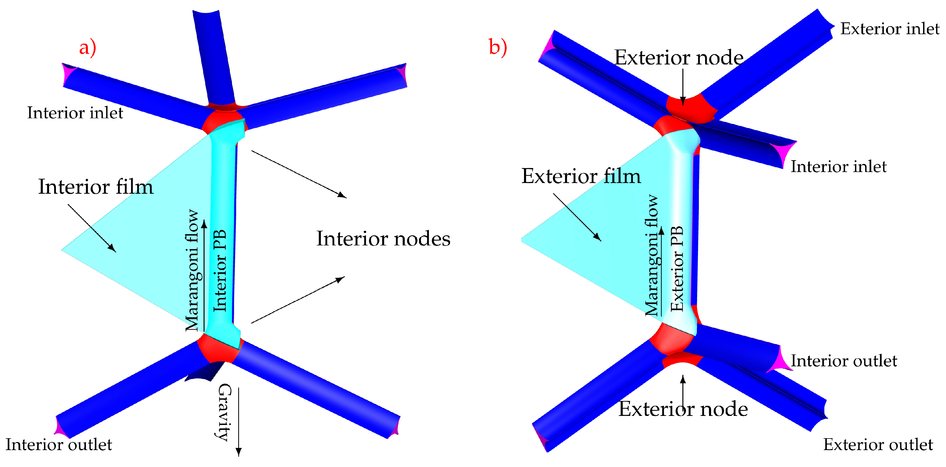
4.3. Effect of Film Thickness on Marangoni Flow

The influence of the film thickness and surface mobility on the liquid velocity of the film was previously studied by Koehler et al. [5] However, they ignored the effect of the Marangoni flow in their calculation for the sake of simplicity. In this research, the Marangoni flow was considered in the surface flow of the film and investigated for different film thicknesses and interface mobilities. The results are presented in Figure 8a,b for interior and exterior foams, respectively.
As discussed by Anazadehsayed et al. [39] and shown in Figure 8, the node–PB velocity decreased slightly with increasing film thickness. This is owing to the slight increase in the zero-velocity conjunction of the PB with the film. However, this was not the case for Marangoni flows, particularly for interior foams. The Marangoni flow in mobile liquid–air interfaces decreased considerably in thicker films. This is again owing to the characteristics of the Marangoni flow as a surface-only flow. For the Marangoni flow, the surface force derived from the surface surfactant gradient must overcome the body force of the film ( ρ g ). The body force increased as the film thickness increased, thereby resulting in a weaker Marangoni flow. In exterior foams, as mentioned previously, the presence of a wall is a dominant factor in Marangoni flows, which reduces the effect of film thicknesses.
Following the works of Koehler et al. [5] and Anazadesayed et al. [39], both B o numbers and film thicknesses scaled by the inverse radius of curvature of the PB (Table 2) were combined with the new parameter Λ 1 = B o + w , where w is the dimensionless thickness. Using this dimensionless value, which represents both the interfacial mobility and film thickness, a master curve was developed to determine the scaled Marangoni velocity for any given B o number and film thickness. As shown in Figure 9, the Marangoni velocity in the master curves decreased by Λ 1 increment. However, when the Bo number increased regardless of the film thickness, the Marangoni flow decreased. The scaled velocities of Marangoni flows in Figure 9 are sketched for both interior and exterior foams. However, the scaled Marangoni velocities for a range of Λ 1 collapsed well into master curves in the interior foam (Figure 9a). The master curves for the exterior foams (Figure 9b) had a larger gap between the Marangoni velocity profiles for different thicknesses. This velocity difference in the master curve was visible between the fitted line and lowest thickness. This may be attributed to the presence of a wall in the exterior geometry and surface-only feature of the Marangoni flow, as explained above. Hence, for the exterior foam (based on the results shown in Figure 9b), the gap should be considered for the prediction of Marangoni velocities, particularly for thinner films.

5. Conclusions

The validated model successfully reproduced the Marangoni eye phenomenon. Additionally, the scaled velocities of the Marangoni flows together with those of node–PBs were investigated for interior and exterior foams. This study acknowledges that the Marangoni flow velocities increased when the mobility of the liquid–air interfaces increased for the interior and exterior. Furthermore, a difference between the Marangoni flow trends of the interior and exterior foam was observed. The ratio of Marangoni to PB velocity in the exterior foam was almost constant for both rigid and mobile foams. For the interior foams, however, the ratio was higher in mobile foams than in rigid foams. This is owing to the nature of the Marangoni flow in being a surface-only flow compared to the node–PB, which is a surface-bulk flow. In the mobile interfaces of the interior foams, the Marangoni flow and node–PB flow were on a similar scale as both faced low hydraulic resistances, whereas in more rigid interfaces, the hydraulic resistance of the Marangoni flow was greater than that of the node PB. The effect of the film thickness on the Marangoni flow was also investigated, which showed that the Marangoni flow is more affected by the film thickness compared to the node–PB (this is again owing to the nature of Marangoni flow as an surface-only flow). For thicker films, the Marangoni flow decreased considerably owing to the higher ratio of the body force to the surface-driven flow. Finally, master curves were developed to show the combined effect of the interfacial mobility and film thickness on the Marangoni flow velocity. This curve enabled the calculation of the Marangoni flow velocity for any given interfacial mobility and film thickness.
In conclusion, the results of this study provide valuable insights into the behavior of Marangoni flows in both interior and exterior foams, and the implications of these findings are significant for various industries. Based on these findings, it is recommended that future research investigate how Marangoni flow can act as a controller for manipulating soft particles and producing controlled collisions between them, particularly in the development of microfluidic devices [40,41]. Additionally, exploring the behavior of Marangoni flow in different systems, such as foam fractionation [17] or UV exposure [20], could lead to the development of new methods for controlling foam stability and improving industrial processes. Overall, this research opens up exciting possibilities for further investigation and innovation in the field of foam behavior and control.

Author Contributions

Conceptualization, N.R. and J.A.; methodology, N.R.; software, N.R. and J.A.; validation, N.R.; formal analysis, N.R.; investigation, N.R.; writing—original draft preparation, N.R.; writing—review and editing, N.R., J.A. and J.N.; visualization, N.R.; supervision, J.A. and J.N. All authors have read and agreed to the published version of the manuscript.

Funding

The publication fee for this research received funding from Swinburne University Technology Scholarship (Australian Government RTP Scholarship).

Data Availability Statement

Not applicable.

Conflicts of Interest

We declare there is no conflict of interest. We confirm that there is no role of the funders in the design of the study; in the collection, analyses or interpretation of data; in the writing of the manuscript; or in the decision to publish the results.

Appendix A

Figure A1. Mesh used for numerical simulation of the interior of the foam with film thickness of 5 μ m. The image shows a 3D view of the computational mesh used for the simulation, consisting of 90k number of elements. To generate the mesh, the GAMBIT software was used to create a tetrahedral mesh, which was then imported into AVL FIRE for simulation.
Fluids 08 00113 g0a1
Figure A2. The exterior foam is in contact with the wall, as indicated by the bubbles touching the wall in the ZX plane.
Fluids 08 00113 g0a2

References

  1. Hill, C.; Eastoe, J. Foams: From nature to industry. Adv. Colloid Interface Sci. 2017, 247, 496–513. [Google Scholar] [CrossRef] [PubMed] [Green Version]
  2. Li, R.; Yang, W.; Li, S.; Han, G.; Ma, C. Foam Mobility Control for Surfactant Enhanced Oil Recovery. SPE J. 2008, 15, 928–942. [Google Scholar] [CrossRef] [Green Version]
  3. Simjoo, M.; Dong, Y.; Andrianov, A.; Talanana, M.; Zitha, P.L.J. CT Scan Study of Immiscible Foam Flow in Porous Media for Enhancing Oil Recovery. Ind. Eng. Chem. Res. 2013, 52, 6221–6233. [Google Scholar] [CrossRef]
  4. Yang, J.; Jovancicevic, V.; Ramachandran, S. Foam for gas well deliquification. Colloids Surf. A 2007, 309, 177–181. [Google Scholar] [CrossRef]
  5. Koehler, S.; Hilgenfeldt, S.; Stone, H. Foam drainage on the microscale. J. Colloid Interface Sci. 2004, 276, 420–438. [Google Scholar] [CrossRef]
  6. McKeon, B.J.; Durbin, P.A. The drainage of a foam lamella. J. Fluid Mech. 2002, 458, 379–406. [Google Scholar]
  7. Anazadehsayed, A.; Naser, J. A combined CFD simulation of Plateau borders including films and transitional areas of liquid foams. Chem. Eng. Sci. 2017, 166, 11–18. [Google Scholar] [CrossRef]
  8. Nguyen, A. Liquid Drainage in Single Plateau Borders of Foam. J. Colloid Interface Sci. 2002, 249, 194–199. [Google Scholar] [CrossRef]
  9. Vitasari, D.; Grassia, P.; Martin, P. Surfactant transport onto a foam lamella. Chem. Eng. Sci. 2013, 102, 405–423. [Google Scholar] [CrossRef]
  10. Wang, Z.; Narsimhan, G. Model for Plateau border drainage of power-law fluid with mobile interface and its application to foam drainage. J. Colloid Interface Sci. 2006, 300, 327–337. [Google Scholar] [CrossRef]
  11. Fournier, J.; Cazabat, A. Tear of a Disjoining Marangoni Film. EPL (Europhys. Lett.) 1992, 20, 517. [Google Scholar] [CrossRef]
  12. Myers, T.G. Thin Films with High Surface Tension. SIAM Rev. 1998, 40, 441–462. [Google Scholar] [CrossRef] [Green Version]
  13. Schick, C. A Mathematical Analysis of Foam Films; Shaker Verlag GmbH: Duren, Germany, 2004; Volume 1, Chapter 1. [Google Scholar]
  14. Ghosh, P. Colloid and Interface Science; Prentice-Hall Of India Pvt. Limited: Kolkata, India, 2009; Volume 1, Chapter 2. [Google Scholar]
  15. Bureiko, A.; Trybala, A.; Kovalchuk, N.; Starov, V. Current applications of foams formed from mixed surfactant-polymer solutions. Adv. Colloid Interface Sci. 2015, 222, 670–677. [Google Scholar] [CrossRef] [PubMed]
  16. Leonard, R.A.; Lemlich, R. A study of interstitial liquid flow in foam. Part II. Experimental verification and observations. AIChE J. 1965, 11, 25–29. [Google Scholar] [CrossRef]
  17. Martin, P.; Dutton, H.; Winterburn, J.; Baker, S.; Russell, A. Foam fractionation with reflux. Chem. Eng. Sci. 2010, 65, 3825–3835. [Google Scholar] [CrossRef]
  18. Stevenson, P.; Jameson, G.J. Modelling continuous foam fractionation with reflux. Chem. Eng. Process 2007, 46, 1286–1291. [Google Scholar] [CrossRef]
  19. Grassia, P.; Ubal, S.; Giavedoni, M.D.; Vitasari, D.; Martin, P.J. Surfactant flow between a Plateau border and a film during foam fractionation. Chem. Eng. Sci. 2016, 143, 139–165. [Google Scholar] [CrossRef] [Green Version]
  20. Chevallier, E.; Saint-Jalmes, A.; Cantat, I.; Lequeux, F.; Monteux, C. Light induced flows opposing drainage in foams and thin-films using photosurfactants. Soft Matter 2013, 9, 7054–7060. [Google Scholar] [CrossRef] [Green Version]
  21. Pitois, O.; Louvet, N.; Rouyer, F. Recirculation model for liquid flow in foam channels. Eur. Phys. J. E 2009, 30, 27. [Google Scholar] [CrossRef]
  22. McMillan, L.; Brown, C.; Garcia, A.; Hughes, M.; Kuhlman, T.; Matsui, Y.; Moya, R.; Lujan, W.; Rader, C.; Coker, J. Sandia National Laboratories. 2010; pp. 1–135. Available online: http://prod.sandia.gov/techlib/access-control.cgi/2010/107501.pdf (accessed on 13 February 2023).
  23. Lucassen-Reynders, E.; Cagna, A.; Lucassen, J. Gibbs elasticity, surface dilational modulus and diffusional relaxation in nonionic surfactant monolayers. Colloids Surf. A 2001, 186, 63–72. [Google Scholar] [CrossRef]
  24. Weaire, D.; Hutzler, S. The Physics of Foams; Oxford University Press: Oxford, UK, 1999. [Google Scholar]
  25. Zhu, Y.; Aref, H. Dynamics of two-dimensional foam structures. J. Fluid Mech. 2002, 467, 289–311. [Google Scholar]
  26. Durian, D. Foam mechanics at the bubble scale. Phys. Rev. Lett. 1995, 75, 4780–4783. [Google Scholar] [CrossRef] [PubMed] [Green Version]
  27. Anazadehsayed, A.; Rezaee, N.; Naser, J. Numerical modelling of flow through foam’s node. J. Colloid Interface Sci. 2017, 504, 485–491. [Google Scholar] [CrossRef]
  28. Stevenson, P.; Li, X. A viscous-inertial model of foam drainage. Chem. Eng. Res. Des. 2010, 88, 928–935. [Google Scholar] [CrossRef]
  29. Kallendorf, C.; Cheviakov, A.F.; Oberlack, M.; Wang, Y. Conservation laws of surfactant transport equations. Phys. Fluids 2012, 24, 102105. [Google Scholar] [CrossRef] [Green Version]
  30. Stone, H.A. Convective-diffusion equation for surfactant transport along a deforming interface. Phys. Fluids Fluid Dyn. 1990, 2, 111–112. [Google Scholar] [CrossRef]
  31. Slattery, J.C.; Sagis, L.; Oh, E.-S. Interfacial Transport Phenomena; Springer: New York, NY, USA, 2013. [Google Scholar]
  32. Wong, H.; Rumschitzki, D.; Maldarelli, C. On the surfactant mass balance at a deforming fluid interface. Phys. Fluids 1996, 8, 3203–3204. [Google Scholar] [CrossRef] [Green Version]
  33. Leonard, R.A.; Lemlich, R. A study of interstitial liquid flow in foam. Part I. Theoretical model and application to foam fractionation. AIChE J. 1965, 11, 18–25. [Google Scholar] [CrossRef]
  34. Durand, M.; Langevin, D. Physicochemical approach to the theory of foam drainage. Eur. Phys. J. E 2002, 7, 35–44. [Google Scholar] [CrossRef]
  35. Carrier, V.; Destouesse, S.; Colin, A. Foam drainage: A film contribution? Phys. Rev. E 2002, 65, 061404. [Google Scholar] [CrossRef]
  36. Cohen-Addad, S.; Hohler, R.; Pitois, O. Flow in Foams and Flowing Foams. Annu. Rev. Fluid Mech. 2013, 45, 241–267. [Google Scholar] [CrossRef]
  37. Koehler, S.; Hilgenfeldt, S.; Weeks, E.; Stone, H. Foam drainage on the microscale II. Imaging flow through single Plateau borders. J. Colloid Interface Sci. 2004, 276, 439–449. [Google Scholar] [CrossRef] [PubMed]
  38. Koehler, S.A.; Hilgenfeldt, S.; Weeks, E.R.; Stone, H.A. Drainage of single Plateau borders: Direct observation of rigid and mobile interfaces. Phys. Rev. E 2002, 66, 040601. [Google Scholar] [CrossRef] [PubMed] [Green Version]
  39. Anazadehsayed, A.; Rezaee, N.; Naser, J. Exterior foam drainage and flow regime switch in the foams. J. Colloid Interface Sci. 2018, 511, 440–446. [Google Scholar] [CrossRef] [PubMed]
  40. Kumar, D. A Microfluidic Device for Producing Controlled Collisions between Two Soft Particles. Ph.D. Thesis, University of Toronto, Toronto, ON, Canada, 2016. [Google Scholar]
  41. Motagamwala, A.H. A Microfluidic, Extensional Flow Device for Manipulating Soft Particles. Ph.D. Thesis, University of Toronto, Toronto, ON, Canada, 2013. [Google Scholar]
Figure 1. Geometry of the (a) Interior foam, (b) Exterior foam including two red-colored nodes and one blue-colored interior PB, and an interior film. Inlets/outlets are represented by the pink colors. The exterior nodes are made up of a conjunction of three exterior PBs with an angle of 120 , where two PBs are attached to the wall, with one being perpendicular to the wall. In both geometries, the flow enters from the top of three PB inlets and exits from the three outlets at the bottom. In both geometries, the direction of the gravity force (in the z direction of a coordinate system) is assumed in the opposite direction of the Marangoni flow, which is shown in the interior geometry (a).
Fluids 08 00113 g001
Figure 2. Scaled velocity profiles of different grid densities are shown for 80 k, 90 k and 95 k cells along a line from the PB to the center of the film, which contained three different regions for the PB, transitional area (where Marangoni flow appears), and film. The velocity in the transitional area in the film was dominated by the Marangoni effect and had the highest value in the opposite direction of the gravity force. The color scale shown in the sketched cross-section represents the velocity value where the positive direction is assumed along the gravitation direction. By comparing the velocities to different grids, no significant difference between the results of 90 k and 95 k was seen. Hence, the flow behavior in the net was independent of the grid densities for grids 90 k and higher.
Fluids 08 00113 g002
Figure 3. The velocity of the Marangoni flow versus the average velocity of the flow in the channel (PB) [21]. The blue line represents the fitted line for different experimental velocities, which are measured for different film thickness (different flow rates) by Pitois et al. [21]. As shown, our simulation and experiments for the thinner films corresponded.
Fluids 08 00113 g003
Figure 4. PB velocity validations in the interior and exterior of the foam. The bold line in both the exterior and interior cross-sections represent the specific lengths of the PB (perpendicular to gravitation), where the flow velocities were calculated by Koehler et. al [37,38]. The velocities were compared to those in previous studies and they corresponded.
Fluids 08 00113 g004
Figure 5. Validation of the average velocity dependence of Bo numbers for PB [8], PB-node [27], and node–PB–node systems.
Fluids 08 00113 g005
Figure 6. (a) Marangoni flow stream lines for an interior thin geometry (b) Marangoni eye, wherein red spots represent the maximum velocity of the Marangoni flow in transitional areas.
Fluids 08 00113 g006
Figure 7. (a) Influence of Bo numbers on both the Marangoni and PB velocities for interior foam. The resulting curve corresponded with the experiments [21]. (b). Influence of Bo numbers on the Marangoni and PB velocities in the exterior foam.
Fluids 08 00113 g007
Figure 8. PB and Marangoni velocity in different film thickness are simulated in different Bo number for (a) interior films and (b) exterior films.
Fluids 08 00113 g008
Figure 9. Dimensionless Marangoni velocities for different film thicknesses and Bo number ( Λ 1 ) for (a) interior (b) exterior foams. The velocity values for the different film thicknesses are represented by symbols, and the approximation (fitted line) is represented by the solid curve. In the exterior of the foam (b), the simulated data points with different thickness have quite different Λ 1 , and the fitted line is estimated for all simulated data points. Therefore, it is possible to observe some deviations from the fitted line for some of the data points, particularly for those with different thickness. Therefore, to accurately reflect the uncertainties in the data, error bars have been added.
Fluids 08 00113 g009
Table 1. Geometry and Simulation Parameters. The approximate Reynolds number of the flow for the chosen radius of curvature and thin films is less than 1 [28]. Hence, in most numerical studies of very dry foams, the Stokes equation is solved using the governing equation. * It is noteworthy that A is the cross-section area which varies in the interior and exterior of the foam for different thicknesses.
ParametersSymbolsValuesUnit
Film thickness α 1, 2.5, 5 μ m
Film length L film 800 μ m
PB length L PB 1000 μ m
Liquid viscosity μ 0.001 Pa   s
Surface areaA* m 2
Gibbs parameterG0.01 N m 1
Fluid density ρ 1000 kg / m 3
Radius of curvature of the Plateau BorderR100 μ m
Initial surfactant surface concentration of the upper stream Γ + 1.1 × 10 6 mol m 2
Initial surfactant surface concentration of the lower stream Γ 0.9 × 10 6 mol m 2
Table 2. Dimensionless parameters [7,9].
ParametersSymbolFormula
Scaled velocity V V / ( ρ A g μ )
Scaled length L L / L f i l m
Bo numberBo μ s / μ R
Scaled surfactant surface concentration Γ Γ / Γ e q
Scaled film thicknessw α / R
Composite parameter Λ 1 B o + w
Disclaimer/Publisher’s Note: The statements, opinions and data contained in all publications are solely those of the individual author(s) and contributor(s) and not of MDPI and/or the editor(s). MDPI and/or the editor(s) disclaim responsibility for any injury to people or property resulting from any ideas, methods, instructions or products referred to in the content.

