Article

Adjoint-Based High-Fidelity Concurrent Aerodynamic Design Optimization of Wind Turbine

1
Department of Mechanical & Aerospace Engineering, School of Engineering and Digital Sciences, Nazarbayev University, Astana 010000, Kazakhstan
2
Department of Mathematics, School of Humanities and Sciences, Nazarbayev University, Astana 010000, Kazakhstan
3
Department of Civil, Environmental and Mining Engineering, The University of Western Australia, 35 Stirling Highway, Crawley, WA 6009, Australia
4
Key Laboratory of Ocean Energy Utilization and Energy Conversion of Ministry of Education, Dalian University of Technology, Dalian 116024, China
*
Author to whom correspondence should be addressed.
Fluids 2023, 8(3), 85; https://doi.org/10.3390/fluids8030085
Submission received: 3 January 2023 / Revised: 6 February 2023 / Accepted: 13 February 2023 / Published: 28 February 2023

Abstract

:
To evaluate novel turbine designs, the wind energy sector extensively depends on computational fluid dynamics (CFD). To use CFD in the design optimization process, where lower-fidelity approaches such as blade element momentum (BEM) are more popular, new tools to increase the accuracy must be developed as the latest wind turbines are larger and the aerodynamics and structural dynamics become more complex. In the present study, a new concurrent aerodynamic shape optimization approach towards multidisciplinary design optimization (MDO) that uses a Reynolds-averaged Navier–Stokes solver in conjunction with a numerical optimization methodology is introduced. A multidisciplinary design optimization tool called DAFoam is used for the NREL phase VI turbine as a baseline geometry. Aerodynamic design optimizations in terms of five different schemes, namely, cross-sectional shape, pitch angle, twist, chord length, and dihedral optimization are conducted. Pointwise, a commercial mesh generator is used to create the numerical meshes. As the adjoint approach is strongly reliant on the mesh quality, up to 17.8 million mesh cells were employed during the mesh convergence and result validation processes, whereas 2.65 million mesh cells were used throughout the design optimization due to the computational cost. The Sparse Nonlinear OPTimizer (SNOPT) is used for the optimization process in the adjoint solver. The torque in the tangential direction is the optimization’s merit function and excellent results are achieved, which shows the promising prospect of applying this approach for transient MDO. This work represents the first attempt to implement DAFoam for wind turbine aerodynamic design optimization.

1. Introduction

Due to the potential for wind energy to be accessible worldwide and its sustainability, it is one of the most prominent alternatives to conventional fossil energy. To improve the aerodynamic and mechanical performance of wind energy, as well as increase the amount of energy collected by wind turbines, optimizing the blade design is critical. Though, due to the sophisticated nature of the aerodynamics and the interaction of the air with the blade structure, optimizing the blade design is a highly challenging aspect of wind turbine optimization. As a result, advanced numerical simulation techniques must be used. Currently, wind turbine design optimization software, such as Ansys [1], OpenFOAM [2], Fast [3], Open Fast [4], QBlade [5], PreComp and BModes [6], Flex 5, and Matlab [7] are utilized, while in certain studies XFoil [8] and AirfoilPrep are used to simulate the aerodynamics of the blades. To attain the desired lift and drag coefficients necessary to generate maximum power, determining the optimal angle of attack at each span section is critical, as are the shape of the airfoil, twist in the blade, and thickness of the airfoil throughout the span. One of the most effective methods of optimization is to divide the blades into multiple portions along their span and examine their overall aerodynamic qualities using numerical simulation techniques. Because the primary goal of the current wind turbine blade design is to minimize the cost and weight and simultaneously increase the energy collection efficiency by the wind turbine with deformation constraints, multidisciplinary concurrent optimization of aerodynamic and structural components and the fluid–structure interaction should be used [9].
As one of the most critical components of a wind turbine, the turbine blade is critical for improving power production which is also exposed to complex external aerodynamic stresses [10]. The optimization of the blade is divided into two branches: structural optimization and aerodynamic optimization [11]. Aerodynamic optimization is concerned with the optimal aerodynamic design, loads, and noise levels, as well as the produced power efficiency, while structural optimization is concerned with weight, mechanical performance such as bending rigidity/strengths and fatigue life span, and so on.
An ideal optimization procedure would include both branches as an optimization goal when numerous objectives are considered. However, intricate research settings and processes make it difficult for researchers to choose these branches rather than simplifying the procedure and optimizing two branches sequentially. While the majority of studies investigate either structural or aerodynamic optimization, others explore the combination of the two [12,13,14,15,16]. In terms of aerodynamic optimization, most of the work has been carried out using BEM rather than CFD (see below for more details). As a result, high-fidelity aerodynamic design optimization is critical for optimizing wind turbines. The current study performed concurrent high-fidelity full shape optimization, planform design optimization, and pitch angle optimization, and produced and described the optimal solutions in detail.

2. Literature Review

2.1. Low-Fidelity Aerodynamic Design Optimization

The aerodynamic design of a wind turbine rotor, as a highly critical aspect in wind turbine design, entails determining the rotor shape and forecasting the rotor’s aerodynamic performance. Numerous computational methodologies, such as blade element momentum (BEM) theory, vortex wake method, and computational fluid dynamics (CFD) have been used to analyze wind turbines’ aerodynamics and their performance. Due to its simplicity and accuracy, the BEM theory is frequently utilized in the aerodynamic design of wind turbines [17]. The BEM theory is based on Glauert’s propeller theory [18]. Robustness, on the other hand, has been a concern with BEM codes, since they do not always converge [19]. Robustness is crucial, even more so when the analysis is performed as part of an optimization process. In the best-case scenario, a lack of resilience will cause the convergence to be slowed down, while in the worst-case scenario, the optimization will be terminated entirely. Ning [20] addressed this problem by re-parameterizing the BEM equations with a single local inflow angle, ensuring convergence. Overall, BEM-based optimization approaches provide excellent results at a low computational cost [21] for certain flow conditions.
Numerous studies on wind turbine blade shape optimization have been conducted. Chehouri et al. [22] conducted an in-depth examination of wind turbine optimization strategies. Ceyhan [23] optimized the aerodynamic performance of horizontal axis wind turbine blades using BEM theory and a genetic algorithm (GA). The distribution of chords and twist angles are treated as design factors and adjusted for maximum power generation.
In the BEM, the blade is assumed to be composed of multiple separate spanwise parts, where the induced velocity at each element is calculated by maintaining a momentum balance on an annular control volume encompassing the blade element. While this model is simple and straightforward to use, it is not accurate enough for many flow conditions since it cannot precisely assess the influence of the wake and sophisticated three-dimensional flows due to its simplistic assumptions.

2.2. High-Fidelity Gradient-Based Aerodynamic Design Optimization

Aerodynamic shape optimization based on high-fidelity CFD simulations has been essential in the field of design optimization during the last two decades. However, it continues to face difficulties related to high computational costs, which may be prohibitively costly when doing a large number of computationally expensive CFD simulations. As a result, it is critical to develop more efficient aerodynamic shape optimization algorithms that can achieve an ideal design with the fewest feasible high-fidelity and costly CFD simulations.
The well-known approaches for optimizing aerodynamic shapes are classed as gradient-based, gradient-free heuristic, and surrogate-based optimization (SBO). Gradient-based methods are very efficient when the gradients are calculated using Jameson’s adjoint technique [24]. The disadvantage is that the optimality of the solution might be very dependent on the initial predictions, and it can get caught in a local minimum [25]. When an efficient gradient assessment is available, gradient-based approaches are preferred. Gradient-based optimization was pioneered in the 1970s with gradients generated using finite-difference approximations [26]. With an increasing number of design variables, the cost of this calculation becomes too expensive. To overcome this problem, adjoint techniques were proposed which enable the evaluation of gradients at a cost that is independent of the number of design variables. Peter and Dwight [27] discussed these and more techniques for calculating aerodynamic shape derivatives. Martins and Hwang [28] expanded the adjoint approach and studied its relationship with various methods of derivative assessment.
As an alternative to the gradient-free heuristic technique, metaheuristic optimization algorithms such as GA, simulated annealing, or particle swarm algorithm have strong global optimization capabilities. When used for aerodynamic shape optimization, however, this sort of technique often takes thousands of CFD simulations or perhaps more, and the whole computing cost may quickly surpass the allotted computational budget. As a result, their applications have often been limited to two-dimensional aerodynamic configurations or three-dimensional configurations employing low-fidelity and quick CFD modeling techniques [13,29,30,31,32]. Surrogate-based optimization (SBO) [33] is a class of optimization methods that use low-cost surrogate models to mimic costly objective and constraint functions, directing the addition and assessment of fresh sample points toward the global optimum. Nonetheless, when the number of design variables increases, the computing cost of optimization increases fast and quickly becomes prohibitively expensive.
Gradient-based algorithms are the only option for design optimization with a large number of variables if one intends to achieve convergence to an optimum in a reasonable length of time [34]. The performance of this method is highly reliant on the cost and precision of calculating the gradients. While finite differences are easy-to-implement methods for computing gradients, they are prone to numerical errors and scale poorly with the number of design variables [35]. Since high-fidelity aerodynamic shape optimization models are driven by a system of non-linear partial differential equations (PDEs), performing an accurate differentiation of the system of PDEs is quite difficult. This is one of the reasons for the scarcity of results from high-fidelity gradient-based aerodynamic shape optimization.
Pironneau [36] proposes an adjoint technique in fluid mechanics, and Jameson [24] expanded it for aerodynamic shape optimization. Since then, the adjoint approach has been extensively employed in gradient-based optimization for aerodynamics applications [37]. There are two distinct techniques to construct the adjoint equations for a primal solver based on the partial differential equations (PDEs): continuous and discrete techniques [38]. The continuous technique uses the adjoint formulation of the governing equations from the original ones and then discretizes them for the numerical solution. The early work of Anderson and Venkatakrishnan [39], as well as the earliest adjoint implementations in OpenFOAM [40], all used this method. Continuous adjoints are more efficient and need less memory than the discrete adjoints. However, the accuracy of the continuous adjoint method degrades on coarse meshes [41].
At the moment, there are few studies on the high-fidelity aerodynamic shape optimization of wind turbine blades. However, one effort has been made to solve the NREL VI wind turbine blade using a RANS solver and a continuous adjoint technique [42]. Dhert et al. [43] and Madsen et al. [44] have recently published exceptional work on this topic. Dhert et al. [43] employed a discrete adjoint solver to perform multipoint optimization on a two-bladed rotor with a 2.6 million cell mesh, maximizing the torque coefficient while restricting the pitch, twist, and local shape design factors. Madsen et al. [44] employed a discrete adjoint solver to perform multipoint optimization on a three-bladed rotor with a 14.16 million cells mesh, optimizing pitch, twist, local shape, and chord as design variables while restricting thickness, thrust, and flap-wise bending momentum. While the same method was used in both situations, Madsen et al. used a more memory-efficient reverse automatic differentiation.
By varying the sweeping curve of NREL phase VI, Dias Marcelo et al. [45] produced more current work that outlines an optimization technique. In this study, the validation and optimization were carried out at wind speeds between 5 and 15 m/s and between 10 and 15 m/s, respectively, using the turbulence model k–ω SST. Compared with our study which mainly concentrates on optimization at the speeds of 7 m/s and 10 m/s with torque as an objective function, it is obvious that it is a great example of multipoint optimization with Cp as the objective function.
While the blade shape of the NREL phase VI is optimized in another study by Kaya, M. et al. [46,47] by altering the taper distribution while leaving the blade planform area constant. The root, mid-span, and tip of a cubic spline are fitted in the spanwise direction to produce the taper distribution. The study found that the mid-span chord grows larger than the root chord and the torque rises as the tip chord shrinks. In contrast, to get the greatest torque in our work, the chord length grows from the root to the tip.
Many researchers have employed surrogate models to reduce the computing time required during the design phase of a wind turbine problem since the current trend in aerodynamic optimization is based on neural networks. These models considerably simplify and solve design challenges, including optimization. Common surrogate models include neural networks and the response surface methodology (RSM). In one such study, Kaya, M. et al. [47] adjusted the stacking axes for taper and twist while leaving the taper ratio and twist distribution over the span the same. This transformed the baseline NREL VI rotor blade planform. A 3D RANS CFD solver is used to create different samples and solve them. In comparison with the torque and thrust values of the estimated samples, a surrogate model based on NN is derived. For maximum torque, both restricted and unconstrained optimization techniques are used once the NN model has been established. It is less computationally intensive and more competitive due to its neural network foundation.
Vorspel et al. [48] recently conducted an unconstrained optimization of the NREL Phase VI rotor by altering up to nine twist design factors using the steepest descent optimization technique. They highlighted their concerns over the convergence, which is not surprising given that the turbine is stall-regulated and exhibits split flow at certain intake speeds. Vortices at the tip and root exacerbated the problem of convergence, resulting in poor gradient quality. They solved this problem by restricting the deformable region to the outside 50% of the blade length, hence limiting shape optimization. Our current research builds on the previously described work and implements new improvements. The primary enhancement is the addition of dihedral as a design variable for optimization, which was not previously considered in wind turbine research. The DAFoam software [49,50] is implemented and utilized in this investigation, and it is based on the open-source CFD solver OpenFOAM. To the best of our knowledge, this study represents the first-ever work on wind turbine optimization implementing and using the DAFoam to date based on adjoint and RANS solvers with the reverse reverse-mode automatic differentiation (AD) technique [50].

3. Methodology and Mathematical Modeling

As described above, the entire high-fidelity aerodynamic design optimization is performed using the open-source program DAFoam [49]. The package is built on the Mach-aero framework [49,51], which includes pyOptSparse [52] and pyGeo [53] for optimization, as well as OpenFOAM as a fluid solver. The tool is based on the adjoint technique, a fast method for generating derivatives that enables gradient-based optimization to be applied to the systems with a high number of design variables. Given the large number of design variables and the complexity of the design process, the Sparse Nonlinear OPTimizer (SNOPT) is used [54]. This section details the geometry, mesh generation method, CFD, verification, and validation, as well as the formulation for design optimization.

3.1. RANS Formulations and CFD Methods

3.1.1. Baseline Geometry

The optimization is based on the NREL Phase VI geometry, which was created for applied CFD validation tests. The NREL Phase VI test is a full-scale Unsteady Aerodynamic Experiment (UAE) conducted in the NASA Ames wind tunnel on the two-bladed 10.058 m diameter NREL Phase VI Rotor based on the S809 airfoil [55]. Figure 1 illustrates the baseline geometry of the airfoil, which is re-plotted based on Hand et al. [55].
The design process included rigorous trade-off analyses that examined nonlinear taper and twist distributions, as well as the incorporation of additional airfoils. The outcome is a blade with linear taper and a nonlinear twist distribution that utilizes the S809 airfoil from root to tip. This baseline geometry offers a suitable starting point for optimization while providing the potential for further performance gains.
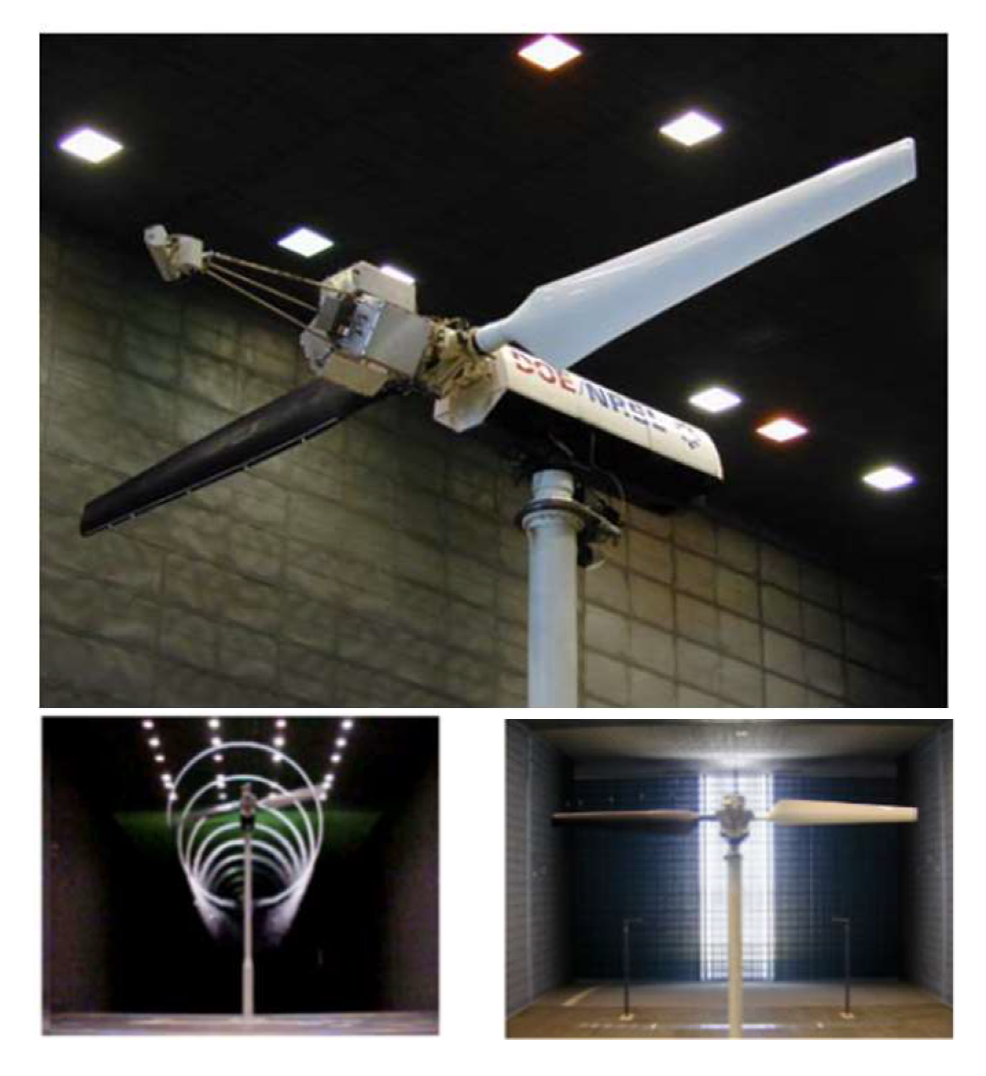
NREL quantified the knowledge on the 3D aerodynamic behavior of full-scale, horizontal-axis wind turbines (HAWT) utilizing the Phase VI wind turbine [55,56]. The NREL Phase VI wind turbine has full-span pitch control and a 20 kW rating. The wind tunnel tests, conducted in 1999 at NASA’s Ames Research Center (Figure 2), are widely regarded as a gold standard for evaluating wind turbine aerodynamic simulation.
For wind speeds ranging from 5 to 25 m/s, a variety of experimental observations were made for blade surface pressures, integrated aerodynamic forces, shaft torque and thrust, blade root strain, tip acceleration, and wake characteristics. This turbine has 2 blades, a 12.2 m hub height and a 10.058 m rotor diameter. The blade profile, which is linearly tapered and nonlinearly twisted, is based on the S809 airfoil profile [57,58]. The NREL study contains detailed information regarding structural geometries, mechanical and material characteristics, as well as experimental findings and methodology [55,56]. In our paper, the trailing edge of the airfoil has been slightly modified to have a higher mesh quality to prevent severe non-orthogonality during mesh generation.

3.1.2. Governing Equations and Boundary Conditions

Since the velocities are relatively low in comparison with the speed of sound and the density does not vary during the flow, it may be inferred that the flow is incompressible. For a three-dimensional steady incompressible flow, the Navier–Stokes equations for mass and momentum conservation are applied as in Equations (1) and (2):
. u = 0 .
u t + . u u = 1 ρ p ¯ + μ . u .
where u is the fluid velocity, p is the pressure, ρ is the density, μ is the fluid dynamic viscosity, and body force does not appear explicitly.
As for the turbulence model used, the one-equation Spalart–Allmaras model [51] is chosen due to its robustness, cheapness, good convergence, and fast implementation, and its boundary conditions are as shown in Table 1. The initial values for k, ε, νt, ω, and ṽ are 0.8375 m2/s2, 0.2 m2/s3, 5 × 10⁻⁵ m2/s, 12.24 s−1 and 5 × 10⁻⁵ m2/s, respectively. The inlet velocity is 7 m / s and the rotational velocity of the blade is 72 rpm.

3.1.3. Mesh Generation and Mesh Convergence Studies

The mesh domain is made up of blades and a fluid domain around them. A meshing program, Pointwise, was utilized to build hybrid meshes across the domain, including completely structural meshes around the blade and non-structural meshes in the farfield domain.
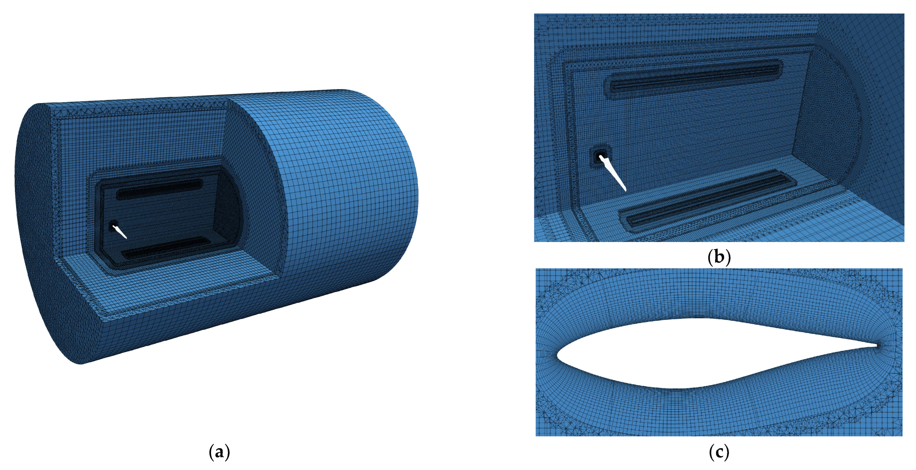
To evaluate the mesh convergence and resolve the wake vortices with sufficient details and improve the accuracy of the CFD results, three levels of grids with varying grid densities are created while maintaining all other parameters constant. These grids are called L0, L1, and L2, respectively. L0 has the finest mesh, L1 a medium mesh, and L2 a coarse mesh. The wind turbine’s medium-sized mesh is seen in Figure 3a,b. To better capture the vortices at the blade’s tip and root, the mesh around these areas were fine-tuned. There are sixty-five layers of boundary layer cells extruded from the turbine surface, as shown in Figure 3c. The growth ratio is 1.2 and the initial cell height away from the turbine surface is set at 0.0005 m to keep the y+ value below 10, where y+ is a non-dimensional distance from the wall to the first mesh node and the superscript cross indicates normalization with the axis that used to be the distance. To be confident in applying a wall function technique to a given turbulence model, y+ values must be guaranteed to fall within a specified range. The blade pressure distribution was examined and converted to sectional aerodynamic force coefficients. To simulate realistic turbulent flow around the blades and to validate the findings, wind tunnel test data are required. Although Reynolds-averaged Navier–Stokes equations (RANS) CFD analysis is more computationally expensive and CFD has limitations, it may be preferable to simulate a wind tunnel test for examining surface pressure distribution. For the whole CFD analysis and optimization, an HPC with 72 processors and 503 GB RAM is utilized.
Multi Reference Frame (MRF) is a steady-state technique used in CFD to describe issues with rotating components. Therefore, disregarding the tower and nacelle should have a minimal impact on the simulation results. As mentioned above, three meshes are used for the mesh convergence study. Table 2 shows the details of the meshes used and the comparison of torque with that obtained from experiments. Although the mesh L0 is the most preferable and accurate one among three sets of mesh levels, due to the computational cost, L2 is chosen for the optimization.
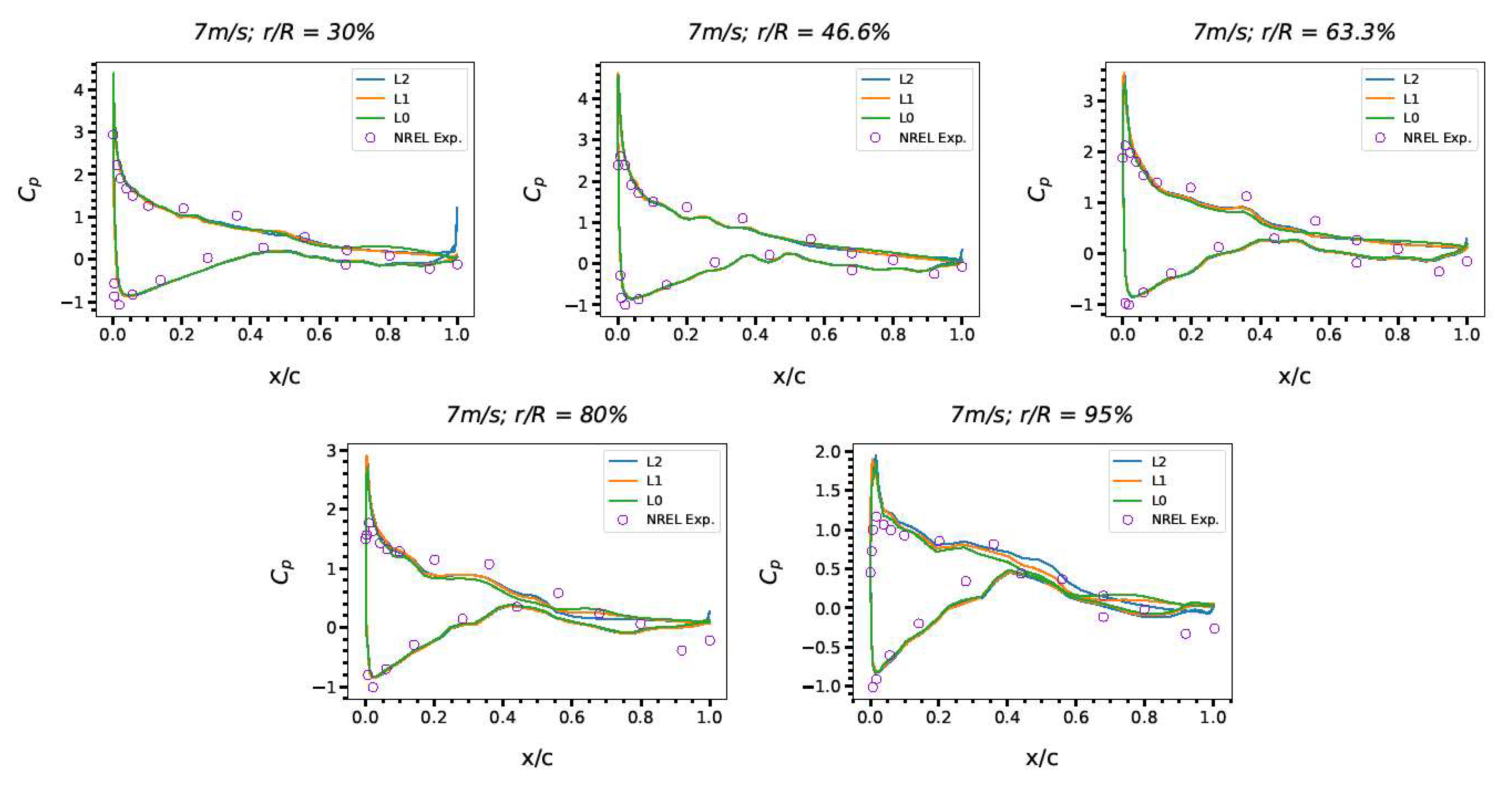
Pressure coefficients (Cp) at various locations along the blade can be computed with Equation (3), where p is the local pressure on the blade surface and p is the atmospheric pressure, and u is the free-stream velocity and ω is the angular velocity. The results of Cp versus x/c for a wind speed of 7 m/s are shown in Figure 4 to validate our CFD analysis against the experimental results reported by NREL [56]. The predicted Cp values agree quite well with the experimental data, especially with the increase in the cell numbers.
C p = p p 0.5 ρ u 2   + ω r 2  
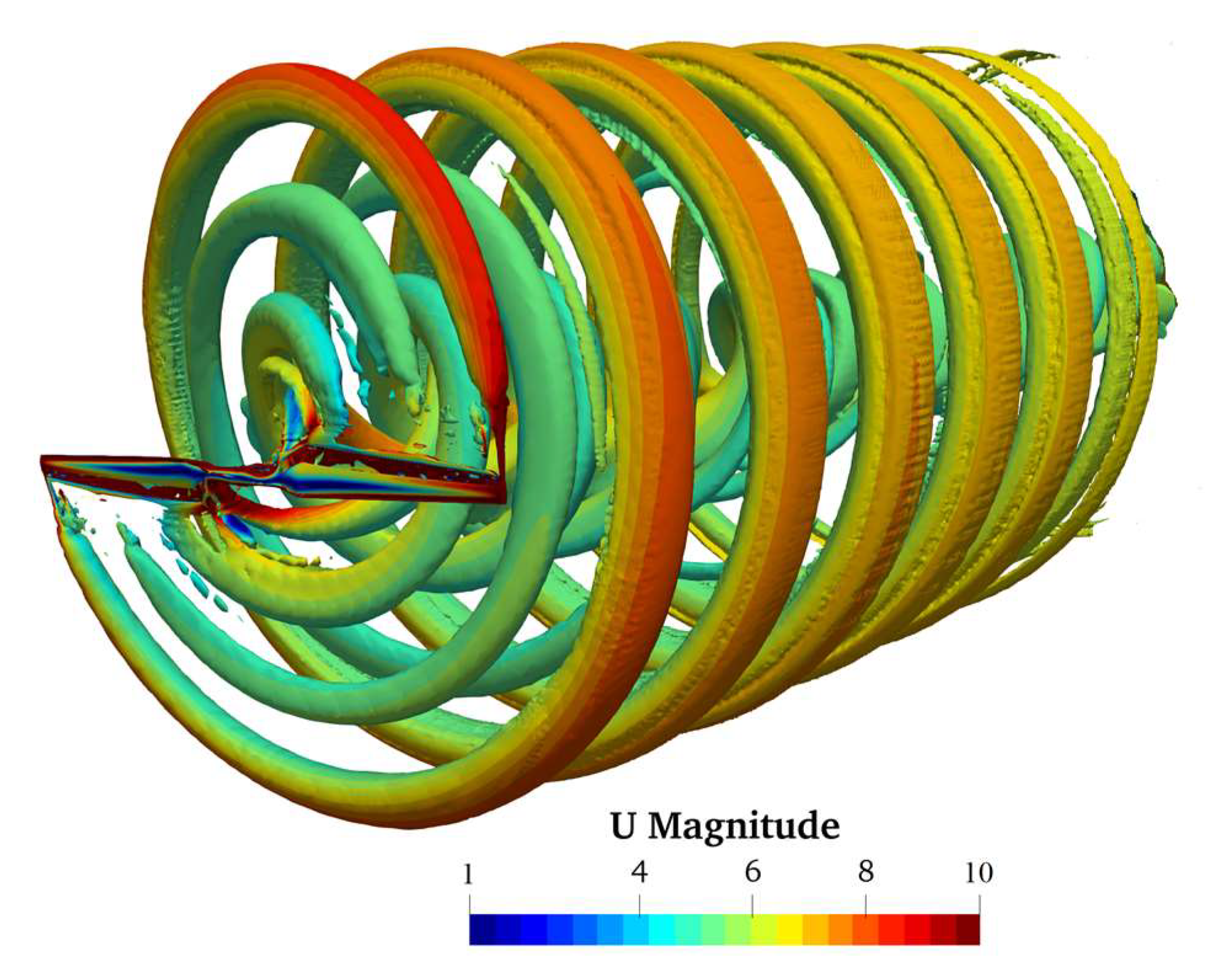
To further verify the mesh quality in the wake region, Figure 5 depicts the helical structure developed by the tip vortices with the fine mesh L0, which shows a uniform distribution and persists for a relatively far distance downwind from the wind turbine rotor.

3.2. Adjoint Equations and Optimization Frameworks Formulation

DAFoam implements the discrete adjoint solver using the FD Jacobian technique [59], which computes all partial derivatives using the coloring-accelerated finite difference method and solves the adjoint equations using the Krylov method. Below, we describe the adjoint equations briefly while most of the processes were explained thoroughly in some works [34,60]. The adjoint approach is used to quickly calculate the total derivatives d f / d x , where f denotes the objective function, which is the torque in our case, and x is the vector of design variables. In the discrete method, it is assumed that the primal solver is capable of generating a discretized version of the governing equations and that the design variable vector x n x and the state variable vector ω n ω meet the discrete residual equations R ω ,   x = 0, where R n ω is the residual vector.
The relevant functions are thus functions of both the design and the state variables: f = R ω ,   x . While there are many functions of interest, in the following derivations, f is treated as a scalar to maintain generality. As will become clear later, each new function necessitates the solution of another adjoint system. The chain rule is used to derive the total derivative d f / d x :
d f d x 1 × n x =   f x 1 × n x   + f ω 1 × n ω d ω d x n ω × n x
where the partial derivatives f / x and f / ω are reasonably straightforward to estimate due to the absence of implicit calculations. On the other hand, the total derivative matrix d ω / d x is costly since it is implicitly defined by the residual equations R ω ,   x = 0.
Using the chain rule for R, we can get d ω / d x . Because the governing equations should always hold, we can then leverage this knowledge to our advantage. As a result, the sum of the derivatives d R / d x must be zero:
d R d x = R x + R ω d ω d x = 0 d ω d x n ω × n x = R ω 1 n ω × n ω R x   n ω × n x
In Equation (5), substituting d ω / d x from Equation (4) yields:
d f d x 1 × n x = f x 1 × n x f ω 1 × n ω R ω 1 n ω × n ω ψ T R x   n ω × n x
Using f / ω T as the right-hand side, we may solve the adjoint equation by transposing the state Jacobian matrix R / ω .
R ω T n ω × n ω ψ n ω × 1   = f ω T n ω × 1
The ψ is the adjoint vector. After solving this equation, we can obtain the total derivative by substituting the adjoint vector into Equation (6), which results in:
d f d x = f x ψ T R ω
For each function of interest, we need to solve the adjoint equations only once because the design variable is not explicitly present in Equation (7). Therefore, its computational cost is independent of the number of design variables, but it is proportional to the number of functions of interest. This approach is known as the adjoint method and has advantages for many aerospace engineering design problems in which there are only a few functions of interest but several hundred design variables may be used.
A discrete adjoint implementation entails calculating the partial derivatives and solving the adjoint equations, and consists of the following four key procedures:
(1) Calculating partial derivatives f / ω T and R / ω T .
(2) Solution of the linear Equation (5) for the adjoint vector ψ .
(3) Computation process of the partial derivatives f / x and R / x .
(4) Using Equation (6) to calculate the total derivative d f / d x .
The aforementioned four procedures can be applied to any set of discrete PDEs since they do not presuppose a particular residual function R ω ,   x .
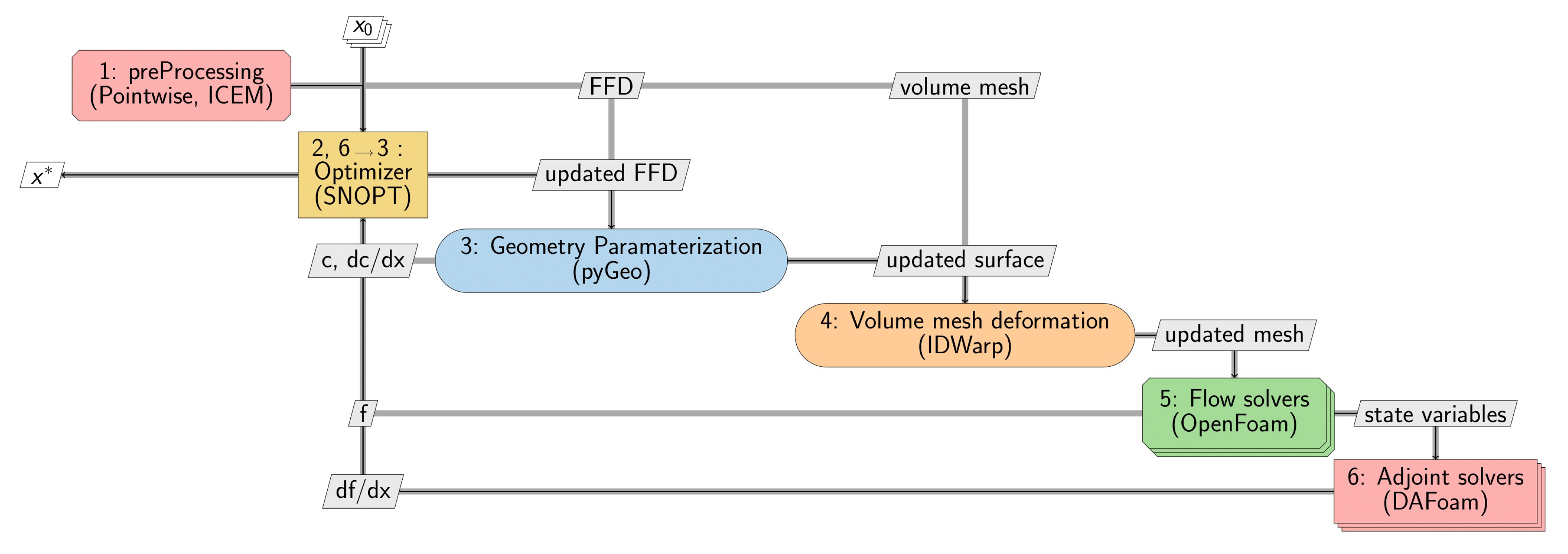
Figure 6 represents the optimization framework created by using the tool extend design structure matrix (XDSM) [61], where the sequence in which components are performed is established by sequentially numbering them beginning with one. Numeric order is used to represent the sequence of execution. The thick gray lines indicate data connections, while the thin black lines indicate process connections. The modules are represented by the diagonal nodes, whereas the data are represented by the off-diagonal nodes. The stacked modules demonstrate parallel operation. The order in each node indicates the sequence of execution:
  • In step 1 (preProcessing), a volume mesh is produced for the baseline geometry using Pointwise, which will be utilized later, as well as free-form deformation (FFD) points using ICEM, which will be used later in step 3 to morph the design surface (geometric parametrization).
  • In step 2, the optimizer (SNOPT) is provided with a collection of baseline design variables. The design variables will be updated and passed along to the geometry parameterization module (pyGeo).
  • Step 3 accepts the updated design variables and FFD points created in the pre-processing phase, executes the deformation for the design surface, and then sends it to the mesh deformation module (IDWarp) for mesh deformation. In addition, pyGeo computes the values of geometric constraints and their derivatives with respect to the design variables.
  • In step 4, IDWarp deforms the volume mesh in accordance with the modified design surface and delivers the deformed volume mesh to the flow simulation module.
  • In step 5, CFD tools (OpenFoam) are used in the flow simulation module to calculate the state variables in process 5 and send them to the adjoint solver.
  • In step 6, the total derivatives of the objective function of the design variables are computed and sent to the optimizer.
  • In the end, SNOPT obtains the values and derivatives of the objective functions and constraints, executes the SQP computation, and returns a collection of updated design variables to pyGeo.
  • The above procedures are repeated until convergence is obtained.

3.3. Geometric Parameterization and Mesh Deformation

The FFD control points are produced using ICEM and then parameterized using pyGeo. As such, FFD embeds the object’s geometry into a volume that may be changed by moving FFD points on the surface. The initial FFD box is constructed with volumetric control points. The design surface is embedded inside the FFD box, and the mapping between the design surface’s physical coordinates and the FFD’s parameter space is constructed. By repositioning the FFD control points, the design surface is distorted.
The number of FFD control points affects an optimization problem’s design flexibility. Thus, the number of FFD control points utilized influences the final design. Generally, 20 points are used for each airfoil segment while optimizing the design.
As seen in Figure 7, the FFD box in this work is 10 × 2 × 15, with 10 × 2 × 7 for each blade and 10 × 2 × 1 for the origin section. Ten control points are located on both the pressure and suction side of each segment throughout the span of each blade’s seven sections, among which one section is fixed and the rest are free to be used for the optimization process. The spanwise direction is x, chordwise direction is y, while the thickness direction of the blade is z.
FFD points are utilized to optimize the local shape, twist, chord length, dihedral, and pitch angle of the blade. Since the blades must be optimized equally and concurrently, they are compelled to undergo the same amount of change due to symmetrical constraints. Three stations are fixed between two blades. Concerning the remaining geometric constraints, volume and thickness constraints are applied, while leading edge (LE) and trailing edge (TE) constraints are added to fix the leading and trailing edges and allow for simultaneous local shape and twist optimization. The reference axis is specified directly by passing the DVGeometry class with a pySpline curve object at 30% from the leading edge.
Pitch optimization requires that all portions twist the same amount, while twist optimization requires that each segment twist separately. During the chord length optimization process, only the chords of the root and tip parts are optimized, and the areas in between are interpolated. In the case of the dihedral, the displacement in the y direction relative to the reference axis is added to the control points. During the entire shape optimization process, shape optimization in the y direction is performed in conjunction with twist, chord length, and dihedral. Constraints on the leading and trailing edges are imposed to prevent the local shape variables from causing a shearing twist.
The points along the inside of the trailing and leading edge are provided to form two lines that completely lie inside the blade and the points along the inside of the leading edge are contained in the leList while the ones along the inside of the trailing edge are contained in the teList. Therefore, the leList and teList form 2D grid points, which are projected onto the upper and lower surface of a triangulated-surface representation of the blade to establish the volume and thickness constraints. The leList and teList points (10 × 15) are used for each blade from the root to the tip. Namely, 10 constraint points from the leading edge to the trailing edge are used at the 15 sections of the blade spanwise. They lie totally inside the blade and are used for the thickness and volume control points.

3.4. Design Optimization Algorithm

In our study, the merit function to maximize is the torque in the y direction with respect to pitch, planform, and full shape optimization. The freestream velocity u = 7 m/s while the rotational velocity ω = 72 rpm. Table 3 shows the optimization combinations for 5 different schemes.
As shown in Table 3, the optimization algorithms are categorized as follows and the optimization is conducted accordingly.
  • Optimization scheme S1: pitch optimization with pitch angle as a single design variable.
  • Optimization scheme S2: shape and twist optimization with 120 shapes in the y direction and 6 twist angles as design variables (126 in total).
  • Optimization scheme S3: shape and chord optimization with 120 shapes in the y direction and 2 chord lengths as design variables (122 in total).
  • Optimization scheme S4: shape and dihedral optimization with 120 shapes in the y direction and 6 dihedrals in the y direction as design variables (126 in total).
  • Optimization scheme S5: twist, chord, and dihedral optimization with 6 twist angles, 2 chord lengths, and 6 dihedrals in the y direction as design variables (14 in total).

4. Results and Discussion

The optimization with mesh L2 is implemented and the results are presented and discussed below. The optimizations with respect to such optimization schemes as S1 (pitch optimization), S2 (shape and twist optimization), S3 (shape and chord optimization), S4 (shape and dihedral optimization), and S5 (twist, chord, and dihedral optimization) are carried out respectively and compared respecting the pre- and post-optimization results.

4.1. S1: Pitch Optimization

During the pitch angle optimization, the FFD points at the six sections along the blade (six twist angles) are controlled as a single design variable to obtain the result as shown in Figure 8. Figure 8a depicts the improvement in the merit function as well as the change in optimality in terms of S1 (pitch), which was achieved after only four iterations. Despite the fact that the improvement in torque is 5.34%, the optimality is less than 0.0002, while the optimality tolerance is 1 × 10⁻⁷.
Figure 8 depicts the improvement in the merit function as well as the change in optimality in terms of S1 (pitch), which was achieved after only four iterations. Despite the fact that the improvement in torque is 5.34%, the optimality is less than 0.0002, while the optimality tolerance is 1 × 10⁻⁷.
The optimization is achieved by changing the pitch angle from 0° to 4.91°, as illustrated in Figure 8a. As previously noted, the increase in torque ranges from 648 Nm to 683 Nm, which represents a 5.34% increase.
The optimization is performed in the S1 (pitch angle) scheme, which results in a simultaneous change in twist along the blade of the same amount, which can be up to 4.91° as shown in Figure 8b. The improvement takes place between the stations from 1.25 m to the tip. Pitch angle is optimized by changing the twist of all the sections along the blade with the same amount simultaneously, which was mentioned in the methodology section.

4.2. S2: Shape and Twist Optimization

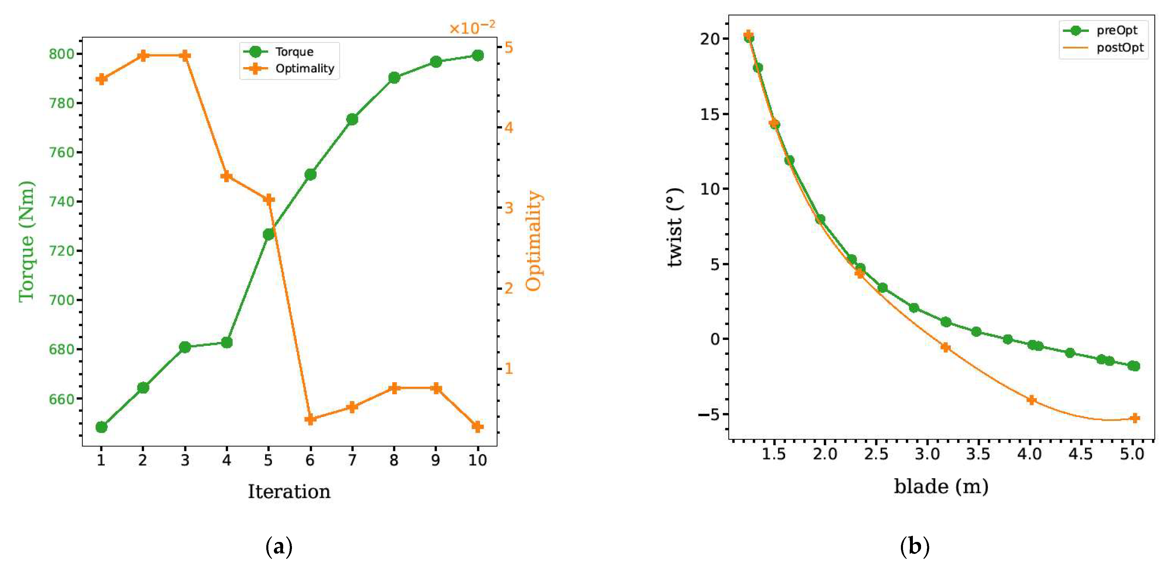
After the pitch angle optimization in S1, the combination of the shape and twist is considered as in S2 for the optimization. In this optimization, 120 (10 × 2 × 6) control points at the 6 stations along each blade for the shape and 6 sections of the FFD points as the design variables along each blade are used. The corresponding results of the optimization are presented in Figure 9a in terms of the objective function (torque), and in Figure 10 the results for Cp before and after the optimization are compared.
Figure 9a presents the merit function improvement as well as the optimality change in terms of S2 (shape and twist), which converged in 10 iterations. The improvement in torque is 23.26% while the optimality reached below 0.01. However, the convergence optimality tolerance for the optimization is 1 × 10⁻⁷, which is much lower than the optimality which occurred for the optimization in our case. As shown in Figure 9b, in optimization scheme S2, both the shape and the twist are improved to lead to the improvement in the merit function and the twist variation along the blade is plotted in orange while the green one presents the twist before the optimization. The twist close to the tip changes substantially compared with the root and the variation is seen by the difference of the twist angle values before and after the optimization in Figure 9b. As sections are optimized in terms of twist along the blade and the sections between them are interpolated accordingly, the location of the six sections is marked in orange on the optimized blade twist profile while the preoptimized twist profile shows twenty marked stations in green along the blade.
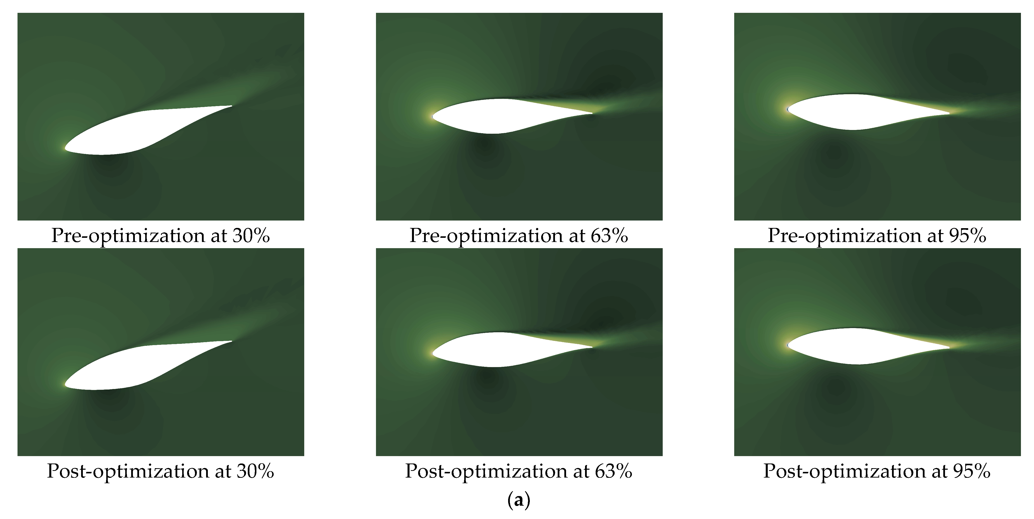
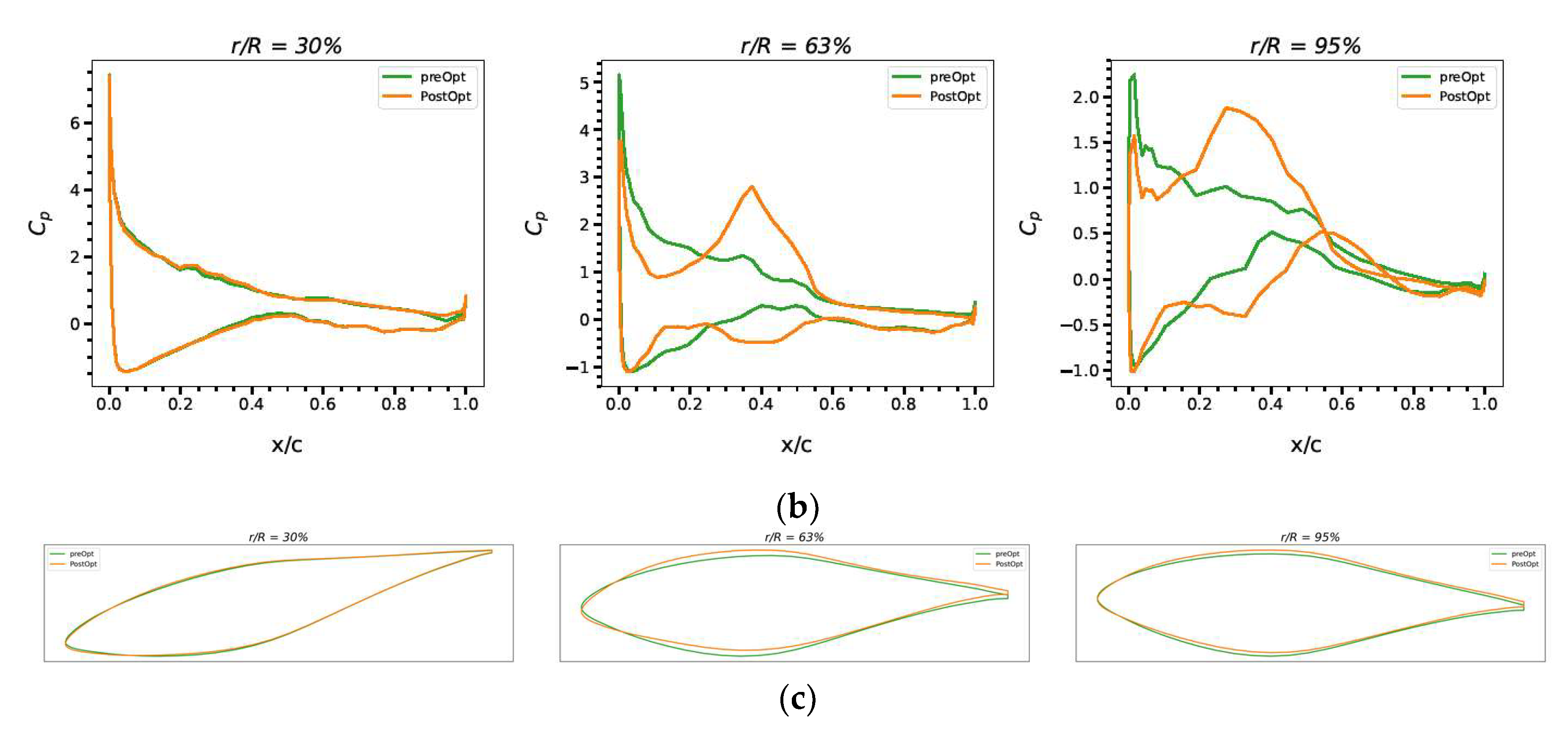
During the optimization, the values of Cp before and after the optimization at 3 stations, i.e., r/R = 30%, 63%, and 95% along the blades are compared in Figure 10b, while the shape profiles of the blade cross section before and after the optimization are presented as well in Figure 10a.
The Cp close to the blade tip (r/R = 95%) is considerable compared with the ones near the root (r/R = 30%) as shown in Figure 10b.

4.3. S3: Shape and Chord Optimization

After the optimizations of S1 (pitch angle) and S2 (shape and twist), the combination of the shape and chord are taken into consideration in S3. During this optimization, 120 (10 × 2 × 6) control points for the shape at the 6 stations along each blade and 2 sections of FFD points as 2 design variables at tip as well as at the root along the blade are utilized.
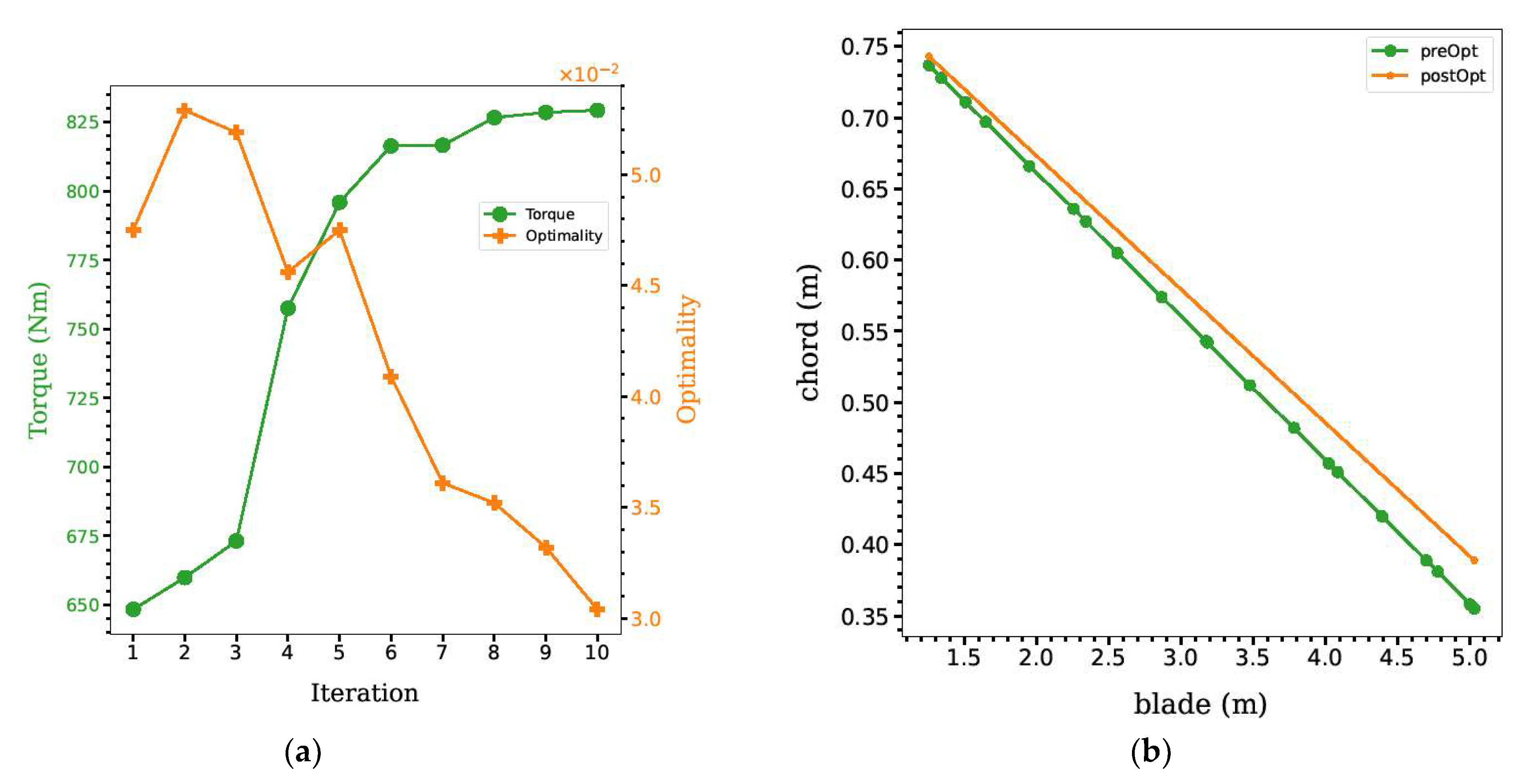
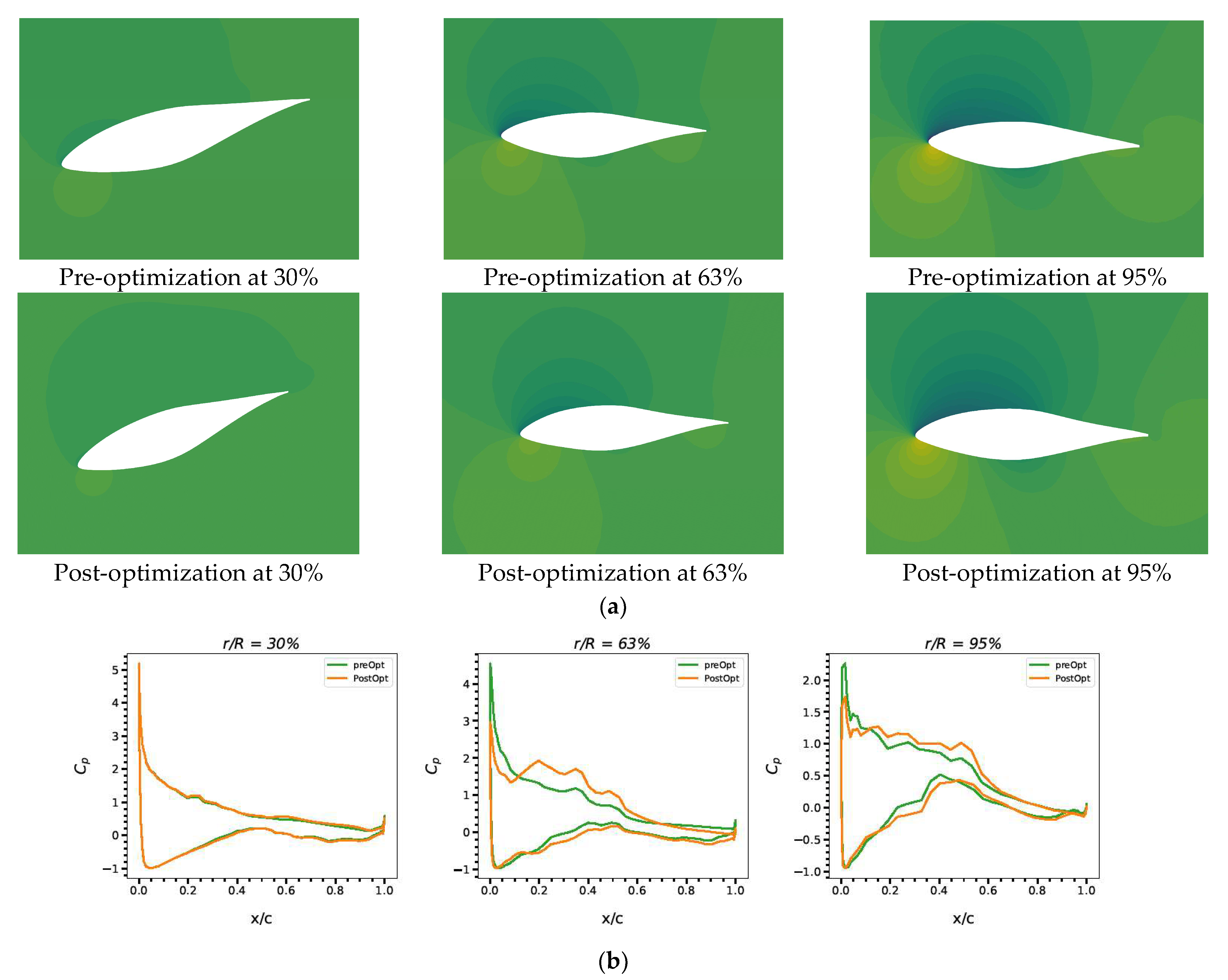
Rather than optimizing shape and twist, in optimization scheme S3 the shape and chord lengths are improved to maximize the objective function torque in the y direction in terms of 120 variables for shape and 2 variables for the chord lengths. Optimization history in terms of the merit function variation and optimality with respect to the iteration sequence is plotted in Figure 11a, while cross-sectional shape profiles as well as the pressure coefficient before and after the improvement at the three sections (i.e., r/R = 30%, 63%, 95%) shown are compared in Figure 12.
It takes 10 iterations to reach the optimization convergence in this case as seen in Figure 11a, where optimality decreases to about 0.02 and the torque increases from 648 Nm to 829 Nm, which is as high as 27.9%. At the end of the third iteration, a sharp growth of approximately 100 Nm in the torque takes place and then it grows gently until the end of the optimization at iteration 10. Observing Figure 11b, the chord length reduces both at the root and the tip as well as at the sections between. The growth in the chord length is around 7.5%.
Comparing Cp values of the pre-optimized and post-optimized blade as presented in Figure 12b, the main changes take place at the regions close to the tip but more or less no changes occur at the root. Considering Figure 12a, the cross-sectional shape profile changes are more obvious at the station r/R = 63%. Furthermore, the change in Cp in the vicinity of the blade tip also accounts for the optimized value of the torque. On the contrary, the changes in the blade root are not as considerable as the ones near the tip. As mentioned earlier, two sections (one at the root and another the tip) are chosen for the chord optimization and thus two design variables for the chord length are varied to obtain the optimum value. The sections between the two sections optimized can be obtained by interpolation.

4.4. S4: Shape and Dihedral Optimization

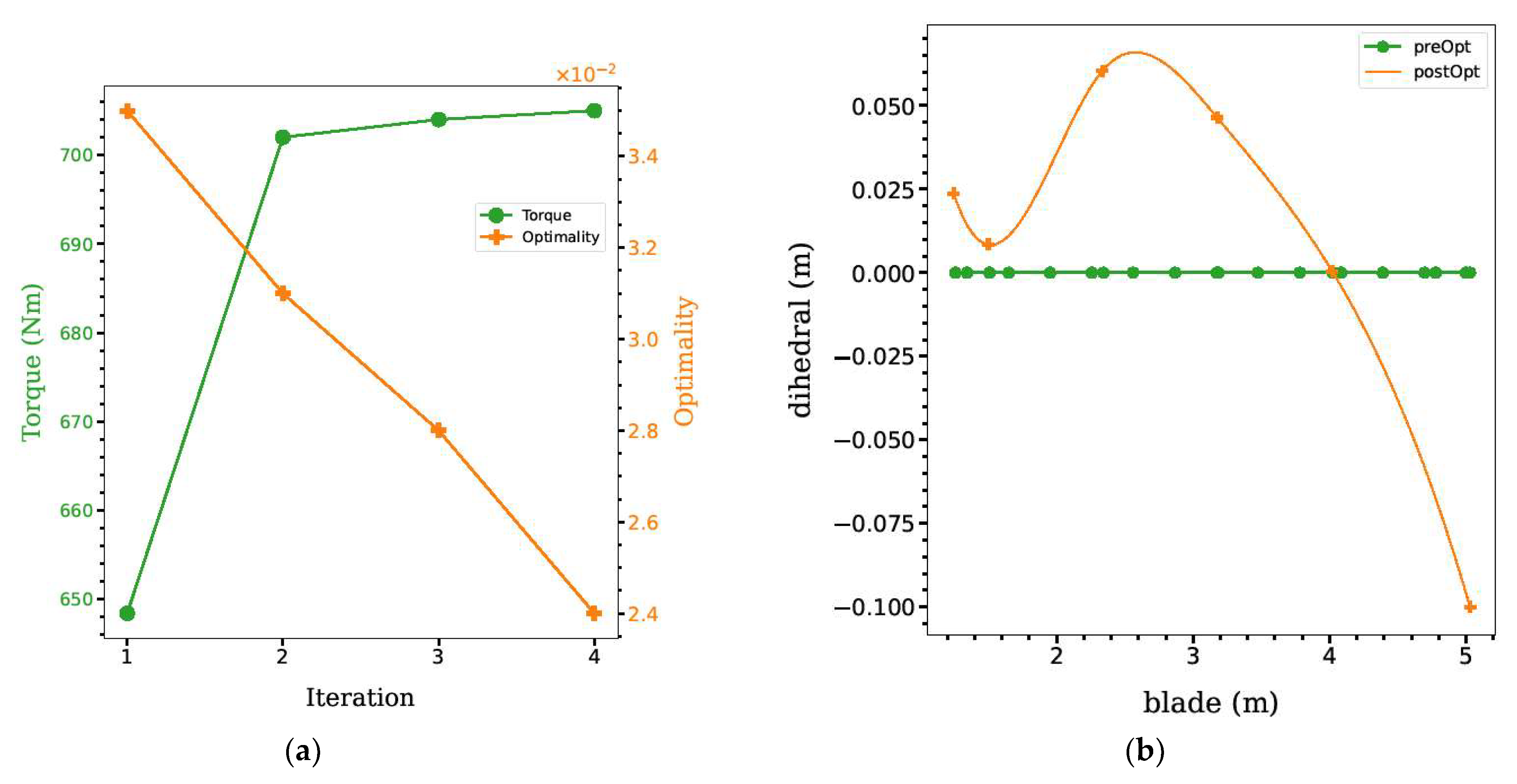
Following the optimization in terms of the combination of shape and twist, and shape and dihedral as in S2 and S3, the combination of shape and dihedral in S4 is examined, and this scheme (S4) consists of 126 design variables in which there are 120 for the shape in the y direction and 6 for the dihedral. The optimization converged with the optimality just below 0.024 and the optimized torque was above 705 Nm (Figure 13a), which represents an increase of 8.7%.
Meanwhile, the dihedral improvement can be found in Figure 13b, where six sections are optimized with corresponding control points marked in orange. Before the optimization, the dihedral value along the blade is zero. The change in the dihedral along the blade is around a few centimeters at the end of the optimization. As only six points are obtained through the dihedral optimization, the rest of the parts are interpolated accordingly. Therefore, a smooth curve is gained as shown in orange in Figure 13b.
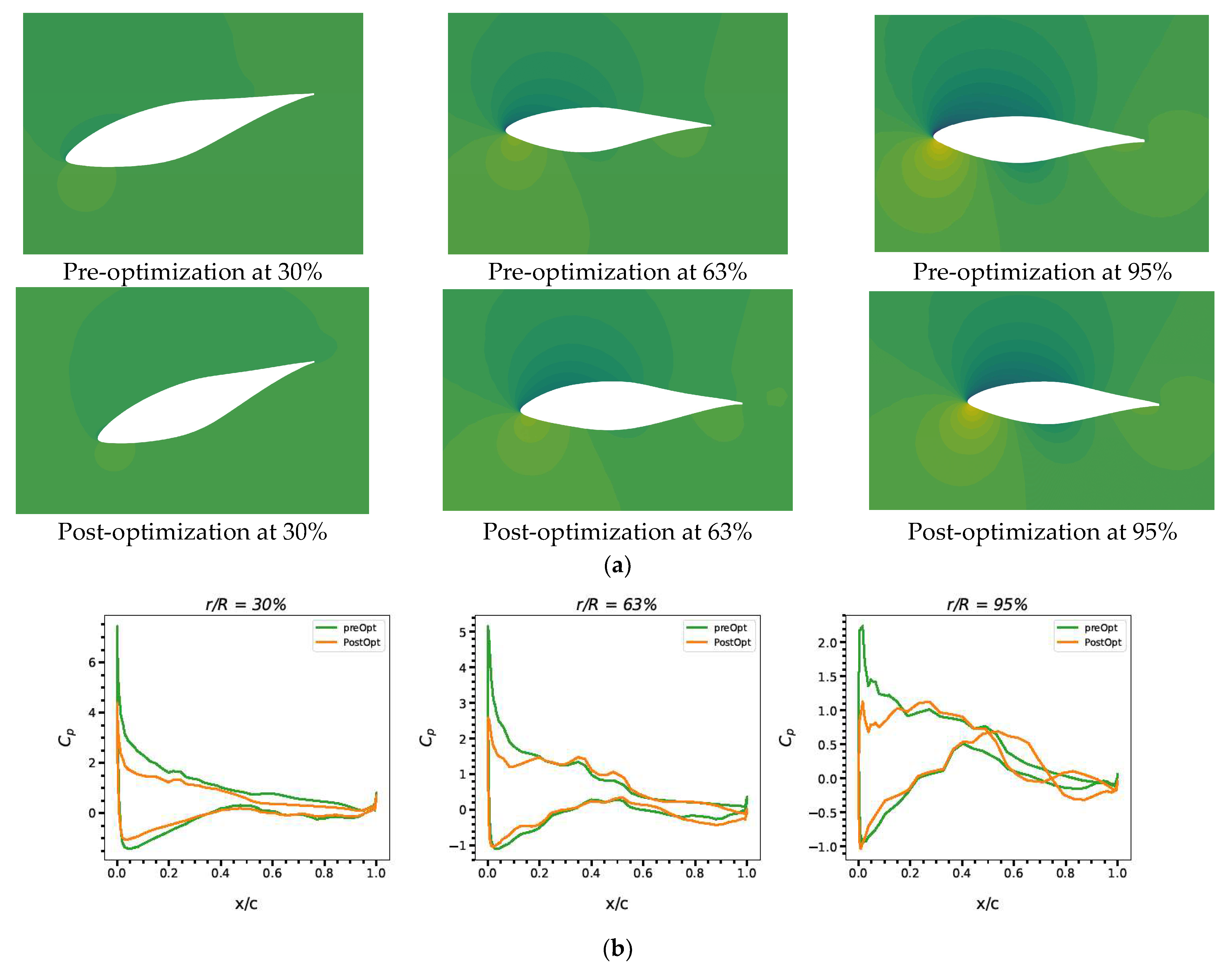
While the optimization in the objective function and dihedral changes are depicted in Figure 13a and in Figure 13b, the Cp at the three stations (i.e., r/R = 30%, 63%, and 95%) are compared with respect to the pre-optimized and post-optimized values as shown Figure 14b.
As shown in Figure 14a, the change in the cross-sectional shape profile of the blade is more obvious at the station r/R = 63%, while the value of Cp varies all over the blade considerably as shown in Figure 14b.

4.5. S5: Twist, Chord, and Dihedral

While in the above sections the combination of the shape and twist, chord length, and dihedral have been taken as the design variables, respectively, in this section the combination of twist, chord lengths, and dihedral are considered for the optimization. At first, we planned to run the full shape optimization which includes local shape and global planform optimization. However, due to the computational cost, we only considered the planform global planform optimization as in this scheme. As for the full shape optimization, we will consider implementing it in the near future.
Usually, twist and chord optimizations are called global planform optimization and the planform optimization for the wind turbine blades was conducted by other researchers without considering dihedral. In this study, dihedral optimization at the six sections is included in the planform optimization apart from the chord length and twist angle optimization, and in this work it is categorized as optimization scheme S5, which has 14 design variables.
In optimization scheme S5, a mere 2.28% increment in torque is achieved (Figure 15a), which is substantially lower in comparison with the optimized values with other schemes discussed above. With this scheme, it takes six iterations to hit the maximum point of the merit function, and the optimality comes to spot slightly above 0.04.
As abovementioned, 14 design variables for the twist angle, chord lengths, as well as the dihedral are taken into account in optimization scheme S5. Examining Figure 15b–d, the crucial change is in the dihedral in contrast to the other factors such as twist and chord lengths which alter marginally to play a part in the optimization of the objective function. Observing Figure 15b,c, the chord and twist undergo a minor difference compared with the baseline, where the change in the twist is around 0.4° and the increase in the chord of the root is 0.0087 m, while the increase in the chord of the tip is around 0.0058 m. As for the little change in the chord and twist compared with the dihedral, the baseline might be close to the optimum value in terms of these two factors by using the low-fidelity methods during the baseline design, which cannot consider 3D effects effectively, such as the dihedral angle. This explains how the optimization mainly happens in the dihedral.
Considering Cp at 3 sections (i.e., r/R = 30%, 63%, and 95%) on the blade prior to, as well as subsequent to, the optimization in Figure 16, the alteration is more significant on the surface nearby both ends while the change is not very obvious in the middle.

5. Concluding Remarks and Further Discussion

The aim of this study is to contribute towards the development of an open source MDO (multidisciplinary design optimization) platform DAFoam in general and develop, implement, and integrate various technologies for wind turbine MDO for the energy community in particular. This work represents the first attempt to implement DAFoam for wind turbine optimization for the wind turbine blades to increase the power output generated.
Three levels of meshes were generated, and verification and validation were performed against the experimental results. Mesh L2 (course mesh/2.6 million) is selected and employed for the optimization due to the high computational cost of finer meshes, while mesh L0 is used for design validation and aerodynamic analysis. The RANS-based high-fidelity concurrent aerodynamic optimization with discrete adjoint method has been successfully demonstrated on the NREL phase VI in terms of five different optimization schemes, namely, S1, S2, S3, S4, and S5, and the results are discussed and compared with the original values.
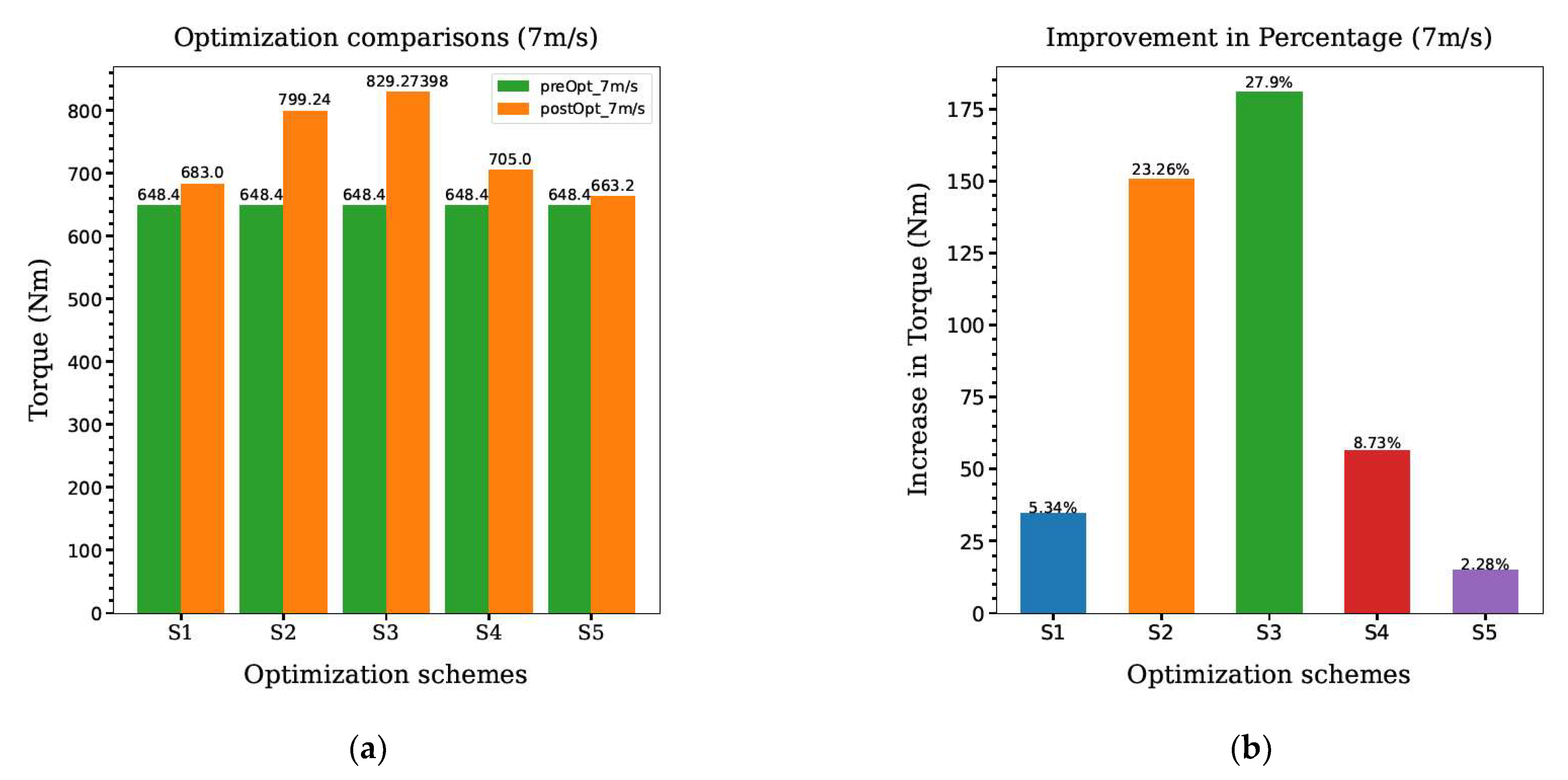
As a conclusion, the merit function values before and after the optimization are compared in Figure 17a with respect to the five optimization methods, where the values prior to the optimization are plotted in orange while the ones after the optimization are plotted in green. The most significant improvement takes place in the optimization schemes S2 and S3, namely, the combination of shape and twist (S2), and shape and chord (S3). Therefore, it can be concluded that the most important aerodynamic parameters to be optimized are the combination of cross-sectional shape, twist, and chord.
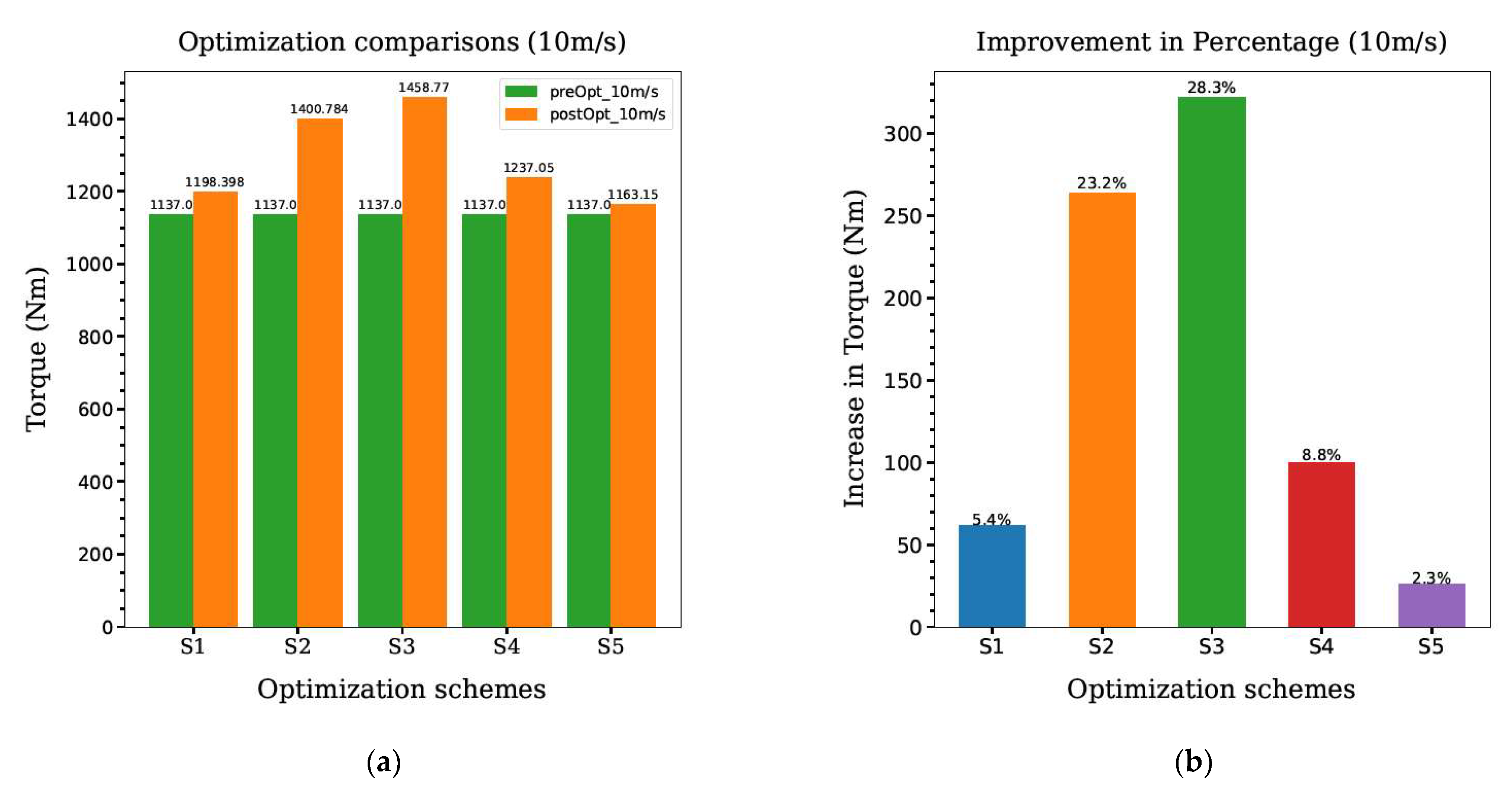
Again, as demonstrated in Figure 17b, the schemes S2 and S3 bring about the most remarkable augmentation in the torque, whereas the insignificant increment takes place with scheme S5. The same optimization schemes for the cases at the inlet velocity of 10 m/s are implemented and the results remain more or less the same as shown in Figure 18. As a part of our future work, multipoint design optimization will be carried out for a range of velocity between 7 m/s and 25 m/s with a certain increment. Since the principal focus of this work is the shape and planform optimization with as many as 135 design variables in all, multidisciplinary (fully aero-structural) design optimization is not taken into account. As a continuation of this work, multidisciplinary design optimization will be pursued with the addition of the solid solver Solid4foam and the TACS VLES (very large eddy simulation) solver.

Author Contributions

Y.Z. oversaw the project and provided the funding as well as the equipment; S.B. developed the geometry, CFD analysis and optimization process, and wrote the manuscript; B.K. and D.Z. assisted with the mesh generation and manuscript; Y.Z., D.W., T.Z. and X.S. reviewed and edited the manuscript. All authors have read and agreed to the published version of the manuscript.

Funding

This study is funded by Nazarbayev University through a FDCR grant No. 240919FD3934 and a FDCR grant No. 20122022FD4126.

Data Availability Statement

Data are available upon request to the first author ([email protected]).

Acknowledgments

The authors would like to thank Nazarbayev University for the financial support for this work through a FDCR grant No. 240919FD3934 and a FDCR grant No. 20122022FD4126.

Conflicts of Interest

The authors declare that they have no conflict of interest.

References

  1. Sagimbayev, S.; Kylyshbek, Y.; Batay, S.; Zhao, Y.; Fok, S.; Soo Lee, T. 3D multidisciplinary automated design optimization toolbox for wind turbine blades. Processes 2021, 9, 581. [Google Scholar] [CrossRef]
  2. Quan, N.N.H.; Van Lam, P. Wind Turbine Blade Design Optimization Using OpenFOAM and DAKOTA Software. Transp. Res. Procedia 2021, 56, 71–78. [Google Scholar] [CrossRef]
  3. Liao, C.; Zhao, X.; Xu, J. Blade layers optimization of wind turbines using FAST and improved PSO Algorithm. Renew. Energy 2012, 42, 227–233. [Google Scholar] [CrossRef]
  4. Chetan, M.; Sakib, M.; Griffith, D.; Gupta, A.; Rotea, M. Design of a 3.4-MW wind turbine with integrated plasma actuator-based load control. Wind. Energy 2022, 25, 517–536. [Google Scholar] [CrossRef]
  5. Altmimi, A.; Alaskari, M.; Abdullah, O.; Alhamadani, A.; Sherza, J. Design and optimization of vertical axis wind turbines using QBlade. Appl. Syst. Innov. 2021, 4, 74. [Google Scholar] [CrossRef]
  6. Sessarego, M.; Ramos-García, N.; Shen, W.Z.; Sørensen, J. Large wind turbine rotor design using an aero-elastic/free-wake panel coupling code. J. Phys. Conf. Ser. 2016, 753, 042017. [Google Scholar] [CrossRef]
  7. Mishnaevsky, L.; Branner, K.; Petersen, H.; Beauson, J.; McGugan, M.; Sørensen, B. Materials for Wind Turbine Blades: An Overview. Materials 2017, 10, 1285. [Google Scholar] [CrossRef] [Green Version]
  8. Akram, M.; Kim, M.-H. CFD analysis and shape optimization of airfoils using class shape transformation and genetic algorithm—Part I. Appl. Sci. 2021, 11, 2211. [Google Scholar] [CrossRef]
  9. Eminoglu, U.; Ayasun, S. Modeling and design optimization of variable-speed wind turbine systems. Energies 2014, 7, 402–419. [Google Scholar] [CrossRef] [Green Version]
  10. Zheng, Y.; Cao, Y.; Zhang, C.; He, Z. Structural Optimization Design of Large Wind Turbine Blade considering Aeroelastic Effect. Math Probl. Eng. 2017, 2017, 1–7. [Google Scholar] [CrossRef] [Green Version]
  11. Burton, T.; Jenkins, N.; Sharpe, D.; Bossanyi, E. Wind Energy Handbook; John Wiley & Sons, Ltd.: Chichester, UK, 2011. [Google Scholar]
  12. Bortolotti, P.; Bottasso, C.; Croce, A.; Sartori, L. Integration of multiple passive load mitigation technologies by automated design optimization—The case study of a medium-size onshore wind turbine. Wind. Energy 2019, 22, 65–79. [Google Scholar] [CrossRef] [Green Version]
  13. Bottasso, C.; Campagnolo, F.; Croce, A. Multi-disciplinary constrained optimization of wind turbines. Multibody Syst. Dyn. 2012, 27, 21–53. [Google Scholar] [CrossRef]
  14. Bottasso, C.; Bortolotti, P.; Croce, A.; Gualdoni, F. Integrated aero-structural optimization of wind turbines. Multibody Syst. Dyn. 2016, 38, 317–344. [Google Scholar] [CrossRef] [Green Version]
  15. Van Kuik, G.; Peinke, J.; Nijssen, R.; Lekou, D.; Mann, J.; Sørensen, J.; Ferreira, C.; van Wingerden, J.; Schlipf, D.; Gebraad, P.; et al. Long-term research challenges in wind energy—A research agenda by the European Academy of Wind Energy. Wind Energy Science 2016, 1, 1–39. [Google Scholar] [CrossRef] [Green Version]
  16. Zhu, J.; Cai, X.; Gu, R. Aerodynamic and structural integrated optimization design of horizontal-axis wind turbine blades. Energies 2016, 9, 66. [Google Scholar] [CrossRef] [Green Version]
  17. Lanzafame, R.; Messina, M. Fluid dynamics wind turbine design: Critical analysis, optimization and application of BEM theory. Renew. Energy 2007, 32, 2291–2305. [Google Scholar] [CrossRef]
  18. Southwell, R.V. The Elements of Aerofoil and Airscrew Theory. By H. Glauert. Pp. 228. 14s. 1926.(Cambridge University Press.). Math. Gaz. 1927, 13, 394–395. [Google Scholar] [CrossRef]
  19. Maniaci, D. An Investigation of WT_Perf Convergence Issues. In Proceedings of the 49th AIAA Aerospace Sciences Meeting Including the New Horizons Forum and Aerospace Exposition, Orlando, FL, USA, 4–7 January 2011; American Institute of Aeronautics and Astronautics: Reston, VA, USA, 2011. [Google Scholar]
  20. Ning, S.A. A simple solution method for the blade element momentum equations with guaranteed convergence. Wind Energy 2013, 17, 1327–1345. [Google Scholar]
  21. Hansen, M. Aerodynamics of Wind Turbines, 2nd ed.; Routledge: London, UK, 2013. [Google Scholar]
  22. Chehouri, A.; Younes, R.; Ilinca, A.; Perron, J. Review of performance optimization techniques applied to wind turbines. Appl. Energy 2015, 142, 361–388. [Google Scholar] [CrossRef]
  23. Ceyhan, Ö. Aerodynamic Design and Optimization of Horizontal Axis Wind Turbines by Using Bem Theory and Genetic Algorithm. Master’s Thesis, Middle East Technical University, Ankara, Turkey, 2008. [Google Scholar]
  24. Jameson, A. Aerodynamic design via control theory. J. Sci. Comput. 1988, 3, 233–260. [Google Scholar] [CrossRef] [Green Version]
  25. Chernukhin, O.; Zingg, D.W. Multimodality and global optimization in aerodynamic design. AIAA J. 2013, 51, 1342–1354. [Google Scholar] [CrossRef] [Green Version]
  26. Hicks, R.; Henne, P. Wing design by numerical optimization. J. Aircr. 1978, 15, 407–412. [Google Scholar] [CrossRef]
  27. Peter, J.; Dwight, R. Numerical sensitivity analysis for aerodynamic optimization: A survey of approaches. Comput. Fluids 2010, 39, 373–391. [Google Scholar] [CrossRef]
  28. Martins, J.R.R.A.; Hwang, J.T. Review and unification of methods for computing derivatives of multidisciplinary computational models. AIAA J. 2013, 51, 2582–2599. [Google Scholar] [CrossRef] [Green Version]
  29. Polat, O.; Tuncer, I. Aerodynamic shape optimization of wind turbine blades using a parallel genetic algorithm. Procedia Eng. 2013, 61, 28–31. [Google Scholar] [CrossRef] [Green Version]
  30. Pourrajabian, A.; Dehghan, M.; Rahgozar, S. Genetic algorithms for the design and optimization of horizontal axis wind turbine (HAWT) blades: A continuous approach or a binary one? Sustain. Energy Technol. Assess. 2021, 44, 101022. [Google Scholar] [CrossRef]
  31. Sun, F.; Xu, Z.; Zhang, D. Optimization Design of Wind Turbine Blade Based on an Improved Particle Swarm Optimization Algorithm Combined with Non-Gaussian Distribution. Adv. Civ. Eng. 2021, 2021, 1–9. [Google Scholar] [CrossRef]
  32. Yang, K. Geometry design optimization of a wind turbine blade considering effects on aerodynamic performance by linearization. Energies 2020, 13, 2320. [Google Scholar] [CrossRef]
  33. Simpson, T.; Poplinski, J.; Koch, P.; Allen, J. Metamodels for computer-based engineering design: Survey and recommendations. Eng. Comput. 2001, 17, 129–150. [Google Scholar] [CrossRef] [Green Version]
  34. Yu, Y.; Lyu, Z.; Xu, Z.; Martins, J.R.R.A. On the influence of optimization algorithm and initial design on wing aerodynamic shape optimization. Aerosp. Sci. Technol. 2018, 75, 183–199. [Google Scholar] [CrossRef]
  35. Martins, J.R.; Sturdza, P.; Alonso, J.J. The complex-step derivative approximation. ACM Trans. Math. Softw. 2003, 29, 245–262. [Google Scholar] [CrossRef] [Green Version]
  36. Pironneau, O. On optimum profiles in Stokes flow. J. Fluid Mech. 1973, 59, 117–128. [Google Scholar] [CrossRef]
  37. ENielsen, J.; Anderson, W. Aerodynamic design optimization on unstructured meshes using the Navier-Stokes equations. AIAA J. 1999, 37, 1411–1419. [Google Scholar] [CrossRef] [Green Version]
  38. Mavriplis, D.J. Discrete adjoint-based approach for optimization problems on three-dimensional unstructured meshes. AIAA J. 2007, 45, 741–750. [Google Scholar] [CrossRef] [Green Version]
  39. Anderson, W.; Venkatakrishnan, V. Aerodynamic design optimization on unstructured grids with a continuous adjoint formulation. Comput. Fluids 1999, 28, 443–480. [Google Scholar] [CrossRef] [Green Version]
  40. Othmer, C. A continuous adjoint formulation for the computation of topological and surface sensitivities of ducted flows. Int. J. Numer. Methods Fluids 2008, 58, 861–877. [Google Scholar] [CrossRef]
  41. Papoutsis-Kiachagias, E.; Giannakoglou, K. Continuous adjoint methods for turbulent flows, applied to shape and topology optimization: Industrial applications. Arch. Comput. Methods Eng. 2016, 23, 255–299. [Google Scholar] [CrossRef]
  42. Economon, T.D.; Palacios, F.; Alonso, J.J. Proceedings of the 21st AIAA Computational Fluid Dynamics Conference, San Diego, CA, USA, 24–27 June 2013; American Institute of Aeronautics and Astronautics: Reston, VA, USA, 2013.
  43. Dhert, T.; Ashuri, T.; Martins, J. Aerodynamic shape optimization of wind turbine blades using a Reynolds-averaged Navier–Stokes model and an adjoint method. Wind. Energy 2017, 20, 909–926. [Google Scholar] [CrossRef]
  44. Madsen, M.H.A.; Zahle, F.; Sørensen, N.N.; Martins, J.R. Multipoint high-fidelity CFD-based aerodynamic shape optimization of a 10 MW wind turbine. Wind. Energy Sci. 2019, 4, 163–192. [Google Scholar] [CrossRef] [Green Version]
  45. Dias, M.M.G.; Ramirez Camacho, R.G. Optimization of NREL phase VI wind turbine by introducing blade sweep, using CFD integrated with genetic algorithms. J. Braz. Soc. Mech. Sci. Eng. 2022, 44, 52. [Google Scholar] [CrossRef]
  46. Kaya, M.; Elfarra, M. Effect of taper distribution on the torque and thrust generated by a wind turbine rotor blade. In Proceedings of the 2019 10th International Renewable Energy Congress (IREC), Sousse, Tunis, 26–28 March 2019; IEEE: Piscataway, NJ, USA; pp. 1–6. [Google Scholar]
  47. Kaya, M.; Elfarra, M. Optimization of the taper/twist stacking axis location of NREL VI wind turbine rotor blade using neural networks based on computational fluid dynamics analyses. J. Sol. Energy Eng. 2019, 141, 011011. [Google Scholar] [CrossRef]
  48. Vorspel, L.; Stoevesandt, B.; Peinke, J. Optimize rotating wind energy rotor blades using the adjoint approach. Appl. Sci. 2018, 8, 1112. [Google Scholar] [CrossRef] [Green Version]
  49. He, P.; Mader, C.A.; Martins, J.R.R.A.; Maki, K.J. An aerodynamic design optimization framework using a discrete adjoint approach with OpenFOAM. Comput. Fluids 2018, 168, 285–303. [Google Scholar] [CrossRef]
  50. He, P.; Mader, C.A.; Martins, J.R.R.A.; Maki, K.J. Dafoam: An open-source adjoint framework for multidisciplinary design optimization with openfoam. AIAA J. 2020, 58, 1304–1319. [Google Scholar] [CrossRef]
  51. Spalart, P.; Allmaras, S. A one-equation turbulence model for aerodynamic flows. In Proceedings of the 30th Aerospace Sciences Meeting and Exhibit, Reno, NV, USA, 6–9 January 1992; American Institute of Aeronautics and Astronautics: Reston, VA, USA, 1992. [Google Scholar]
  52. Wu, N.; Kenway, G.; Mader, C.; Jasa, J.; Martins, J. pyOptSparse: A Python framework for large-scale constrained nonlinear optimization of sparse systems. J. Open Source Softw. 2020, 5, 2564. [Google Scholar] [CrossRef]
  53. Kenway, G.; Kennedy, G.; Martins, J. A CAD-Free Approach to High-Fidelity Aerostructural Optimization. In Proceedings of the 13th AIAA/ISSMO Multidisciplinary Analysis Optimization Conference, Fort Worth, TX, USA, 13–15 September 2010; American Institute of Aeronautics and Astronautics: Reston, VA, USA, 2010. [Google Scholar]
  54. Gill, P.; Murray, W.; Saunders, M. SNOPT: An SQP algorithm for large-scale constrained optimization. SIAM J. Optim. 2002, 12, 979–1006. [Google Scholar] [CrossRef] [Green Version]
  55. Hand, M.; Simms, D.; Fingersh, L.; Jager, D.; Cotrell, J.; Schreck, S.; Larwood, S. Unsteady Aerodynamics Experiment Phase VI: Wind Tunnel Test Configurations and Available Data Campaigns; National Renewable Energy Laboratory: Golden, CO, USA, 2001.
  56. Simms, D.; Schreck, S.; Hand, M.; Fingersh, L. NREL Unsteady Aerodynamics Experiment in the NASA-Ames Wind Tunnel: A Comparison of Predictions to Measurements; NREL: Golden, CO, USA, 2001.
  57. Ramsay, R.; Hoffman, M.; Gregorek, G. Effects of Grit Roughness and Pitch Oscillations on the S809 AirfoilL; NREL: Golden, CO, USA, 1995.
  58. Somers, D.W. Design and Experimental Results for the S809 Airfoil; NREL: Golden, CO, USA, 1997.
  59. Kenway, G.; Mader, C.; He, P.; Martins, J. Effective adjoint approaches for computational fluid dynamics. Prog. Aerosp. Sci. 2019, 110, 100542. [Google Scholar] [CrossRef]
  60. Mader, C.; Martins, J.; Alonso, J.; van der Weide, E. ADjoint: An approach for the rapid development of discrete adjoint solvers. AIAA J. 2008, 46, 863–873. [Google Scholar] [CrossRef]
  61. Lambe, A.B.; Martins, J.R.R.A. Extensions to the design structure matrix for the description of multidisciplinary design, analysis, and optimization processes. Struct. Multidiscip. Optim. 2012, 46, 273–284. [Google Scholar] [CrossRef]
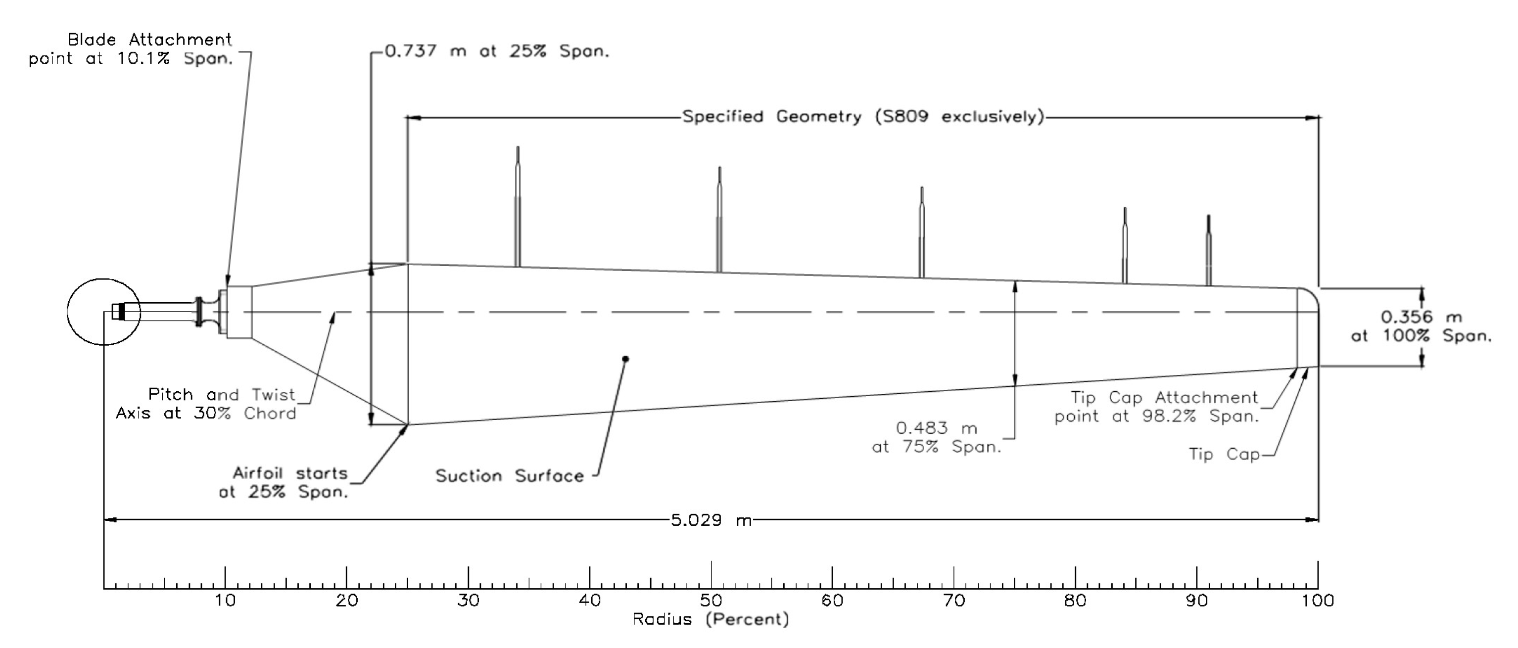
Figure 1. Blade planform dimensions [55].
Fluids 08 00085 g001
Figure 2. NASA’s Ames Research Centre/NREL Phase VI wind turbine [55].
Fluids 08 00085 g002
Figure 3. Mesh formulation: (a) far field mesh layout; (b) mesh cross-section; (c) hyperbolic expansion layer formulation.
Fluids 08 00085 g003
Figure 4. Comparison of the pressure coefficients (Cp) from three levels of mesh (L2, L1, and L0) and NREL Exp.
Fluids 08 00085 g004
Figure 5. Vorticity contour with L0 (fine mesh).
Fluids 08 00085 g005
Figure 6. Optimization framework shown by the extended design structure matrix (XDSM).
Fluids 08 00085 g006
Figure 7. FFD control boxes and points (black) for the optimization.
Fluids 08 00085 g007
Figure 8. (a) Optimization process with respect to S1 (pitch); (b) twist angle variation with respect to S1 (pitch).
Fluids 08 00085 g008
Figure 9. (a) Optimization process with respect to S2 (shape and twist); (b) twist angle variation with respect to S2 (shape and twist).
Fluids 08 00085 g009
Figure 10. (a) Comparison of the cross-sectional shape profile before and after the optimization; (b) comparison of the values for the Cp before and after the optimization in terms of S2 (shape and twist); (c) cross-section change in shape and twist.
Fluids 08 00085 g010aFluids 08 00085 g010b
Figure 11. (a) Optimization process with respect to S3 (shape and chord); (b) chord length variation with respect to S3 (shape and chord).
Fluids 08 00085 g011
Figure 12. (a) Comparison of the cross-sectional shape profile before and after the optimization; (b) comparison of the values for the Cp before and after the optimization in terms of S3 (shape and chord).
Fluids 08 00085 g012
Figure 13. (a) Optimization process with respect to S4 (shape and dihedral); (b) dihedral variation with respect to S4 (shape and dihedral).
Fluids 08 00085 g013
Figure 14. (a) Comparison of the cross-sectional shape profile before and after the optimization; (b) comparison of the values for the Cp before and after the optimization in terms of S4 (shape and dihedral).
Fluids 08 00085 g014
Figure 15. (a) Optimization process with respect to S5 (twist, chord, and dihedral); (b) twist variation with respect to S5 (twist, chord, and dihedral); (c) chord length variation with respect to S5 (twist, chord, and dihedral); and (d) dihedral variation with respect to S5 (twist, chord, and dihedral).
Fluids 08 00085 g015
Figure 16. Comparison of the values for the Cp before and after the optimization in terms of S5 (twist, chord, and dihedral).
Fluids 08 00085 g016
Figure 17. (a) Objective function before and after the optimization for velocity of 7 m/s; (b) improvement in the torque by percentage for the velocity of 7 m/s.
Fluids 08 00085 g017
Figure 18. (a) Objective function before and after the optimization for the velocity of 10 m/s; (b) improvement in the torque by percentage for the velocity of 10 m/s.
Fluids 08 00085 g018
Table 1. Boundary conditions.
Boundary
Conditions
EpsilonNutnuTildakOmegaPU
BladeepsilonWallFunctionnutUSpaldingWallFunctionfixedValuekqRWallFunctionomegaWallFunctionzeroGradientfixedValue
In/outinletOutletfixedValueinletOutletinletOutletinletOutletfixedValueinletOutlet
Table 2. Mesh convergence by comparing the torque result from simulation against experimental value.
Mesh#Mesh TypeCells (106)Torque (Nm)Error (%)
L0Fine mesh17.8577129.2
L1Medium mesh6.31569511.5
L2Course mesh2.657648.417.27
NREL Exp.--785-
Table 3. Optimization algorithms.
Optimization Schemes
Design VariablesNumber of Design VariablesS1S2S3S4S5
Pitch1
Shape120
Twist6
Chord2
Dihedral6
Total 112612212614
Disclaimer/Publisher’s Note: The statements, opinions and data contained in all publications are solely those of the individual author(s) and contributor(s) and not of MDPI and/or the editor(s). MDPI and/or the editor(s) disclaim responsibility for any injury to people or property resulting from any ideas, methods, instructions or products referred to in the content.