Article

Thermal Convection of an Ellis Fluid Saturating a Porous Layer with Constant Heat Flux Boundary Conditions

by
Pedro Vayssière Brandão
1,†,
Michele Celli
1,†,
Antonio Barletta
1,*,† and
Stefano Lazzari
2,†
1
Department of Industrial Engineering, Alma Mater Studiorum Università di Bologna, Viale Risorgimento 2, 40136 Bologna, Italy
2
Department of Architecture and Design, Polytechnic School, University of Genoa, Stradone S. Agostino 37, 16123 Genoa, Italy
*
Author to whom correspondence should be addressed.
These authors contributed equally to this work.
Fluids 2023, 8(2), 54; https://doi.org/10.3390/fluids8020054
Submission received: 19 December 2022 / Revised: 5 January 2023 / Accepted: 31 January 2023 / Published: 2 February 2023

Abstract

:
The present work analyzes the thermal instability of mixed convection in a horizontal porous channel that is saturated by a shear-thinning fluid following Ellis’ rheology. The fluid layer is heated from below by a constant heat flux and cooled from above by the same heat flux. The instability of such a system is investigated by means of a small-disturbances analysis and the resulting eigenvalue problem is solved numerically by means of a shooting method. It is demonstrated that the most unstable modes on the instability threshold are those with infinite wavelength and an analytical expression for such conditions is derived from an asymptotic analysis. Results show that the non-Newtonian character of the fluid has a destabilizing role.

1. Introduction

The study of the Rayleigh–Bénard instability for a fluid-saturated porous layer is a topic of utmost importance for the analysis of convection heat transfer in porous materials. A comprehensive review of this research topic is presented in Nield and Bejan [1]. The literature on this subject is mainly focused on Newtonian fluids. When a non-Newtonian shear-thinning fluid is considered, the Ostwald–De Waele model is frequently employed for the definition of the fluid rheology [2]. Such a model displays a peculiar feature when the shear stress applied to the fluid tends to zero. For this limiting case, the apparent viscosity of the fluid tends to infinity when dealing with pseudoplastic fluids, and to zero for dilatant fluids. This is not always an issue since usually one focuses on non-vanishing mass flow rates of shear-thinning fluids. On the other hand, when dealing with transition to instability, it can be a major problem, as a fluid at rest is a possible basic state for the onset of instability.
In order to fix the singular behavior of the Ostwald–De Waele law, one can employ different rheological models. Nield [3,4] suggested a modified drag force term for Darcy’s law. According to this suggested model, the singularity problem is solved, but only for dilatant fluids. Instead, for pseudoplastic fluids, the problem persists since the apparent viscosity still goes to infinity in the limit of the vanishing shear rate. More recently, Brandao and Ouarzazi [5] and Brandao et al. [6] proposed a modified Darcy’s law based on the Carreau and the Carreau–Yasuda models, respectively. In both cases, the apparent viscosity is reduced to the Newtonian one when the shear stress is negligible. On the other hand, Celli et al. [7] and Brandao et al. [8] proposed the Ellis model as a suitable framework for the description of the rheology of shear-thinning fluids. For the Ellis model, the apparent viscosity is also reduced to the Newtonian one in the absence of shear rate. While the Carreau and Carreau–Yasuda extensions for porous media are recent developments, the Ellis model has been used for a long time in the study of non-Newtonian flow in porous media [9] and is supported by experimental validations.
The pioneering studies on thermal instability in porous media involve Dirichlet boundary conditions for the temperature field, i.e., prescribed temperature at the walls [10,11,12]. Recently, Celli et al. [7] investigated the effect of the shear-thinning characteristics on the thermal instability of an Ellis fluid subject to an unstable temperature gradient due to prescribed temperatures at the walls. It is well-known from the literature that relaxing the Dirichlet boundary conditions for the temperature field leads to a lower critical Rayleigh number for the Newtonian rheology both for clear fluids and for saturated porous media [13,14,15,16]. In addition, such a change in the boundary conditions yields the emergent convective cell to be of larger wavelength (smaller wavenumber). According to Park and Sirovich [14], a smaller value of the Rayleigh number on the instability threshold means a smaller input energy to the fluid and, to accommodate this decrease in the energy, the fluid develops convective cells of infinite wavelength.
The present study aims to investigate the threshold conditions for the onset of thermal convection when a shear-thinning fluid saturates a horizontal porous layer heated from below and cooled from above with the same uniform heat flux. The horizontal boundaries are impermeable and a horizontal throughflow is prescribed. The Ellis model is employed to describe the rheology of the fluid. The stability of a stationary basic state characterized by a uniform flow and a vertical downward temperature gradient is investigated. A linear stability analysis is performed by superposing to the basic state small-amplitude perturbations in the form of normal modes and by solving the eigenvalue problem thus obtained. The aim of this paper is to analyze how the shear-thinning character of the fluid affects the onset of thermal convection.

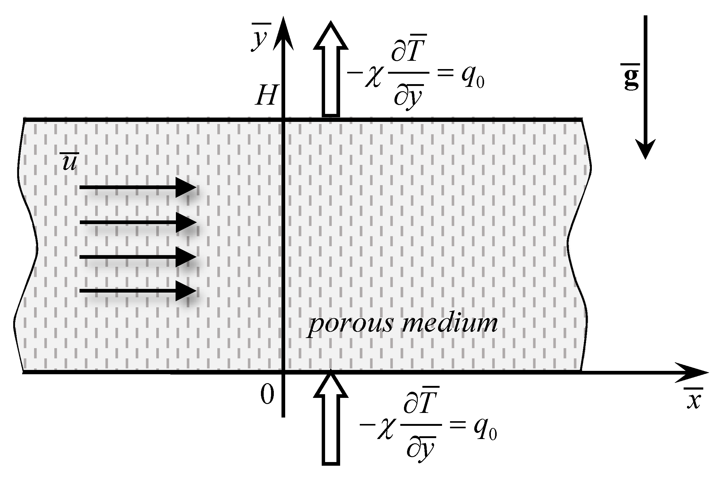
2. Mathematical Formulation

A horizontal porous channel saturated by a shear-thinning fluid is considered. The boundary walls, separated by a height H, are considered to be impermeable and both are subject to a constant heat flux q 0 (see Figure 1). The Oberbeck–Boussinesq approximation is considered and the local thermal equilibrium between the fluid and the solid matrix is assumed. A basic uniform throughflow is imposed along the horizontal x direction.

2.1. Rheological Model

The rheological behavior of the shear-thinning fluid is described by means of the Ellis model. Such a model involves three parameters and describes the rheology of a time-independent, shear-thinning and non-yield-stress fluid [17]. According to the Ellis model, the apparent viscosity η is given by [17,18]:
η = η 0 1 + τ τ 1 / 2 1 a a ,
where a is the Ellis index, η 0 is the apparent viscosity at zero shear-stress and τ 1 / 2 is the value of τ when η = η 0 / 2 . The model is formulated with 0 < a < 1 , although typical values of the Ellis index are within the range 0.14 < a < 0.91 [19].

2.2. Modified Darcy’s Law

The classical version of the Darcy’s law for a Newtonian fluid is given by:
u = K η f d ,
where u represents the seepage velocity vector, whose components are denoted as ( u , v , w ) , K is the permeability of the porous medium and f d is the drag force, which is given by:
f d = p ρ 0 g β ( T T 0 ) ,
where p is the local difference between the pressure and the hydrostatic pressure, ρ 0 is the fluid density at the reference temperature T 0 , g is the gravity acceleration vector and β is the thermal expansion coefficient of the fluid.
A generalized form of Darcy’s law is represented by:
u = K η e f f f d ,
where η e f f is the effective viscosity given by [18]:
1 η e f f = 1 η 0 1 + 4 a 3 a + 1 | f d | r h τ 1 / 2 1 a a ,
with r h being the mean hydraulic radius, which is directly proportional to the square root of the ratio between the permeability K and the porosity φ of the solid medium.
The modified Darcy’s law for a porous medium saturated by a shear-thinning fluid of Ellis type can thus be rewritten as:
u = K η 0 1 + A | f d | 1 a a f d ,
where A is a coefficient that depends on the properties of the fluid and the porous medium.

2.3. Governing Equations

The governing equations for mass, momentum and energy describing the present problem are thus given by:
· u = 0 ,
η 0 K u = 1 + A | f d | 1 a a f d ,
f d = p ρ 0 g β ( T T 0 ) ,
σ T t + u · T = α 2 T ,
y = 0 , H : v = 0 , χ T y = q 0 .
In Equations (10) and (11), σ is the ratio between the average volumetric heat capacity of the porous medium and the volumetric heat capacity of the fluid, and α and χ are the average thermal diffusivity and the average thermal conductivity of the saturated porous medium, respectively.
The following dimensionless quantities, denoted with an overline, are introduced:
x ¯ = x H , u ¯ = H α u , p ¯ = K η 0 α p , t ¯ = α σ H 2 t , T ¯ = T T 0 Δ T ,
where Δ T = q 0 H / χ and x = ( x , y , z ) is the position vector. Furthermore, we define El as the Darcy–Ellis number and R as the Darcy–Rayleigh number, given by:
El = A α η 0 H K 1 a a , R = ρ g β H K Δ T α η 0 .
By substituting Equation (12) into Equations (7)–(11) and by utilizing Equation (13), the governing equations can be written in the following dimensionless form:
· u = 0 ,
u = 1 + El | f d | 1 a a f d ,
T t + u · T = 2 T ,
y = 0 , 1 : v = 0 , T y = 1 ,
where:
f d = p + R T e y .
In Equations (14)–(18), as well as in the forthcoming analysis, the overline symbol for the dimensionless quantities has been omitted for the sake of brevity.
We note that the limit of Newtonian rheology is recovered when El 0 . On the other hand, a very large value of El drives the Ellis model to the power–law model for pseudoplastic fluids. In the latter case, the Ellis index a can be considered as equivalent to the power–law index.

2.4. Basic State

The basic stationary flow is generated by a prescribed constant pressure drop along the x axis, p b / x , and by a prescribed heat flux at the walls. This basic solution is given by:
u b = p b x 1 + El p b x 1 a a , v b = 0 , w b = 0 , p b y = R T b , p b z = 0 , T b = 1 y ,
with b standing for basic state. Without any loss of generality, p b / x can be assumed to be negative to obtain a positive basic velocity u b .
The pressure–temperature formulation of the dimensionless governing Equations (14)–(17) is given by:
· 1 + El | f d | 1 a a f d = 0 ,
T t + 1 + El | f d | 1 a a f d · T = 2 T ,
f d = p + R T e y ,
y = 0 , 1 : p y = R T , T y = 1 .

2.5. Linear Stability Analysis

In order to perform the linear stability analysis, the original fields are decomposed in two parts: one relative to the basic solution and the other one relative to infinitesimal disturbances. Neutral stability conditions, i.e., zero growth rate disturbances, are sought. The linear dynamics of the infinitesimal disturbances is investigated by solving the linearized governing equations. Such disturbances are assumed to behave as plane waves, i.e., Fourier modes, namely:
p ( x , y , z , t ) = p b ( x , y ) + ε f ( y ) e i k x x + k z z ω t , T ( x , y , z , t ) = T b ( y ) + ε h ( y ) e i k x + k z z ω t ,
where ε is a positive small parameter that accounts for the amplitude of the disturbances, f and h are the eigenfunctions of the problem, k x and k z are the wavenumbers in the streamwise and spanwise directions, respectively, and ω is the angular frequency.
After substituting Equation (24) into Equations (20)–(23), the ordinary linear differential equations governing the disturbance dynamics can be written as:
f ˜ a ˜ k 2 f ˜ R ˜ h = 0 ,
h ( k 2 R ˜ i ω ˜ ) h f ˜ = 0 ,
y = 0 , 1 : f ˜ = R ˜ h , h = 0 ,
where the following quantities have been defined:
f ˜ = ( 1 + El ˜ ) f , R ˜ = ( 1 + El ˜ ) R , El ˜ = El p b x 1 a a , k x = k cos ( ϕ ) , k z = k sin ( ϕ ) , ω ˜ = ω k Pe , a ˜ = El ˜ + a ( El ˜ + 2 ) + El ˜ ( 1 a ) cos ( 2 ϕ ) 2 a ( El ˜ + 1 ) .
In Equation (28), Pe is the Pèclet number and the wavenumbers k x and k z are written in terms of a single wavenumber k and the inclination angle ϕ , in order to account for both longitudinal and transverse rolls. It is possible to verify that ω ˜ = 0 , which means that ω = k Pe . In order to demonstrate such a result, let us multiply Equation (25) by the complex conjugate of f ˜ and Equation (26) by the complex conjugate of h and, then, let us integrate the resulting equations over y. By invoking integration by parts and by taking into account the boundary conditions (27), it is possible to show that all terms in the resulting equations are real, which allows us to conclude that i ω ˜ = 0 . In other words, all modes on the instability threshold travel with a phase velocity that is equal to the average velocity of the fluid flow, or equivalently the stability analysis is performed in the comoving reference frame. The Péclet number is not explicitly defined here, but its definition can be recovered by averaging the velocity profile given by Equations (19), namely:
Pe = 0 1 u b d y = p b x 1 + El p b x 1 a a .

3. Asymptotic Analysis for Vanishing Wavenumber

As already mentioned, disturbance modes of a vanishing wavenumber tend to be the most unstable ones on the thermal instability threshold for a fluid layer heated by a constant heat flux. For this reason, it can be useful to investigate the stability of the present problem by focusing on vanishing wavenumbers, i.e., k 0 . In order to do so, an asymptotic analysis is performed here in the vicinity of k = 0 by expanding the eigenfunctions of f ˜ and h, as well as R ˜ , in power series of k and then substituting these series into Equations (25)–(27). Since in Equations (25) and (26) there are only quadratic terms of k, the power series expansions can be performed by considering only quadratic terms, namely:
f ˜ ( y ) = j = 0 k 2 j f ˜ 2 j ( y ) , h ( y ) = j = 0 k 2 j h 2 j ( y ) , R ˜ = j = 0 k 2 j R ˜ 2 j .
After substituting Equation (30) into the original eigenvalue problem represented by Equations (25)–(27), it is possible to solve the problem for each order j. Due to the boundary conditions, h 0 is defined up to a constant. Such a constant is used to fix the solution scale, which allows us to write:
h 0 = 1 ,
while f 0 is given by:
f ˜ 0 = R ˜ 0 y + C 0 ,
where C 0 is an integration constant. With reference to second-order terms, it is possible to obtain the solutions for h 2 and f ˜ 2 :
h 2 = 1 24 a ˜ y 2 R ˜ 0 ( y 2 2 ) + C 0 ( 4 y 6 ) + C 1 ,
f ˜ 2 = R ˜ 2 y + 1 360 y 2 R ˜ 0 a ˜ 60 + R ˜ 0 ( 3 y 5 ) y y 60 R ˜ 0 a ˜ 30 R ˜ 0 ( y 2 ) y + 12 + R ˜ 0 y C 1 + C 2 ,
where C 1 and C 2 are other integration constants. By applying the boundary conditions for f ˜ , given by:
y = 0 , 1 : f ˜ 2 = R ˜ 2 h 0 + R ˜ 0 h 2 ,
it is possible to find the solution for R ˜ 0 :
R ˜ 0 = 12 a ˜ ,
which, written in terms of R 0 and a by employing Equation (28), becomes:
R 0 = 24 a El ˜ + ( El ˜ + 2 ) a + El ˜ ( 1 a ) cos ( 2 ϕ ) .
From Equation (37), one can infer that R 0 is a monotonic increasing function of the inclination angle ϕ . Consequently, the neutral stability condition for k 0 holds for a smaller value of R for transverse rolls. The sensitivity of R 0 to the angle ϕ can be inferred also from the derivative of R 0 with respect to ϕ :
R 0 ϕ = 48 El ˜ ( 1 a ) a sin ( 2 ϕ ) El ˜ + ( 2 + El ˜ ) a + El ˜ ( 1 a ) cos ( 2 ϕ ) 2 .
By considering El ˜ 0 and 0 < a < 1 , Equation (38) always returns positive values in the range 0 ϕ π / 2 . Such a result confirms the monotonicity of R 0 as a function of ϕ , and the transverse modes as the preferred ones for the onset of thermal instability. The results for the most unstable modes can be simplified as follows:
R 0 T = 12 a El ˜ + a ,
where the superscript T stands for transverse. The analytical expression for R 0 considering longitudinal modes is given by:
R 0 L = 12 El ˜ + 1 .
From now on, the present analysis will be focused on the most unstable modes, i.e., the transverse ones. Moreover, it is assumed that ω ˜ = 0 .

4. Results and Discussion

The solution of Equations (25)–(27) was obtained numerically by means of a shooting method, the same as described in Celli et al. [7]. The computations were carried out within the Mathematica environment [20]. The limit El 0 yielded the Newtonian case, whose critical conditions are given by k c = 0 and R c = 12 [1,16]. Table 1 shows a comparison between the present results from the numerical solution for small values of k, and the well-known results for the Newtonian case. The results for k = 0 are those coming from the asymptotic analysis presented in the previous section.
The results are presented in terms of neutral stability conditions, that is, the parametric regime where the disturbances have zero growth rate. Such a condition is expressed by the pair ( k , R ) for prescribed values of the control parameters ( El ˜ , a ) . Figure 2 shows the neutral stability condition for different values of El ˜ and a. One can conclude that the parameter a has a stabilizing effect on the basic state: by increasing a, higher values of R are obtained. Although R can vary noticeably from frame to frame in Figure 2, the trend of the neutral stability curves is similar for the different values of El ˜ shown. Since a controls the shear-thinning character of the fluid, one may affirm that the non-Newtonian character of shear-thinning fluids has a destabilizing effect for the present problem.
One may note that, for a given a, by increasing the value of El ˜ starting from El ˜ = 0 , the basic flow becomes unstable for smaller values of R . In fact, such a result is confirmed by Figure 3. This trend can be physically explained by mentioning that an increment in El ˜ implies an increment in the non-Newtonian character of the fluid flow as well, in analogy to what has been found for the parameter a.
In real-world problems, perturbations of any wavenumber may arise. For this reason, once the smallest R is exceeded in Figure 2, the flow is considered to be unstable, even if it is seemingly stable for values of k larger than the critical wavenumber. By looking at Figure 2, one may deduce that the critical conditions always hold true for k 0 . In fact, Figure 3 illustrates the neutral stability conditions for k = 0.001 and compares it with the asymptotic results given by Equation (39). Thus, we can assume, without any loss of generality, that Equation (39) also expresses the critical conditions:
R c = R 0 T = 12 a El ˜ + a .
Such a conclusion is of great importance since it allows one to obtain the critical conditions entirely analytically. Table 2 shows the critical value of R for the same parametric combination chosen to express the neutral stability condition in Figure 2.
Figure 4 shows a comparison between the neutral stability results for k = 0.001 and the asymptotic solution for k 0 . Such results confirm the trend observed in Figure 2 and suggest again that k = 0.001 can be considered as an approximation of the critical conditions. When El ˜ 0 , the results do not depend on a and coincide with the Newtonian limit. The same can be observed in Figure 2, as the results for El ˜ 0 do not depend on a.
It can be useful to express the critical conditions for the onset of instability in terms of the parameters p b / x , a and El , as follows:
R c = 12 a El p b x 1 a a + a 1 ,
where Equations (28) and (41) have been employed.
Figure 5 shows the dependence of the instability threshold given in terms of R c as a function of the basic pressure gradient. The Newtonian fluid limit ( El 0 ) yields R c = 12 independently of the basic pressure gradient. Thus, Figure 5 shows that R c for a pseudoplastic fluid is always smaller than for a Newtonian fluid. This means that a departure from the Newtonian behavior destabilizes the basic flow. Figure 5 reveals that, for a = 0.8 , there is a marked sensitivity to the basic pressure gradient when p b / x is very small, especially for large values of El .

5. Conclusions

The onset of thermal convection of a shear-thinning fluid saturating a horizontal porous medium subject to constant heat fluxes at its impermeable boundaries was investigated. The Ellis model was considered in order to overcome the singular behavior of the power-law model for vanishing shear rates. A linear stability analysis was performed by considering normal mode disturbances. The most important results can be summarized as follows:
  • There exists a suitable variable transformation that yields a compact representation of the stability eigenvalue problem;
  • The critical conditions hold always for k = 0 . The threshold values can be obtained entirely analytically due to an asymptotic analysis performed for k 0 ;
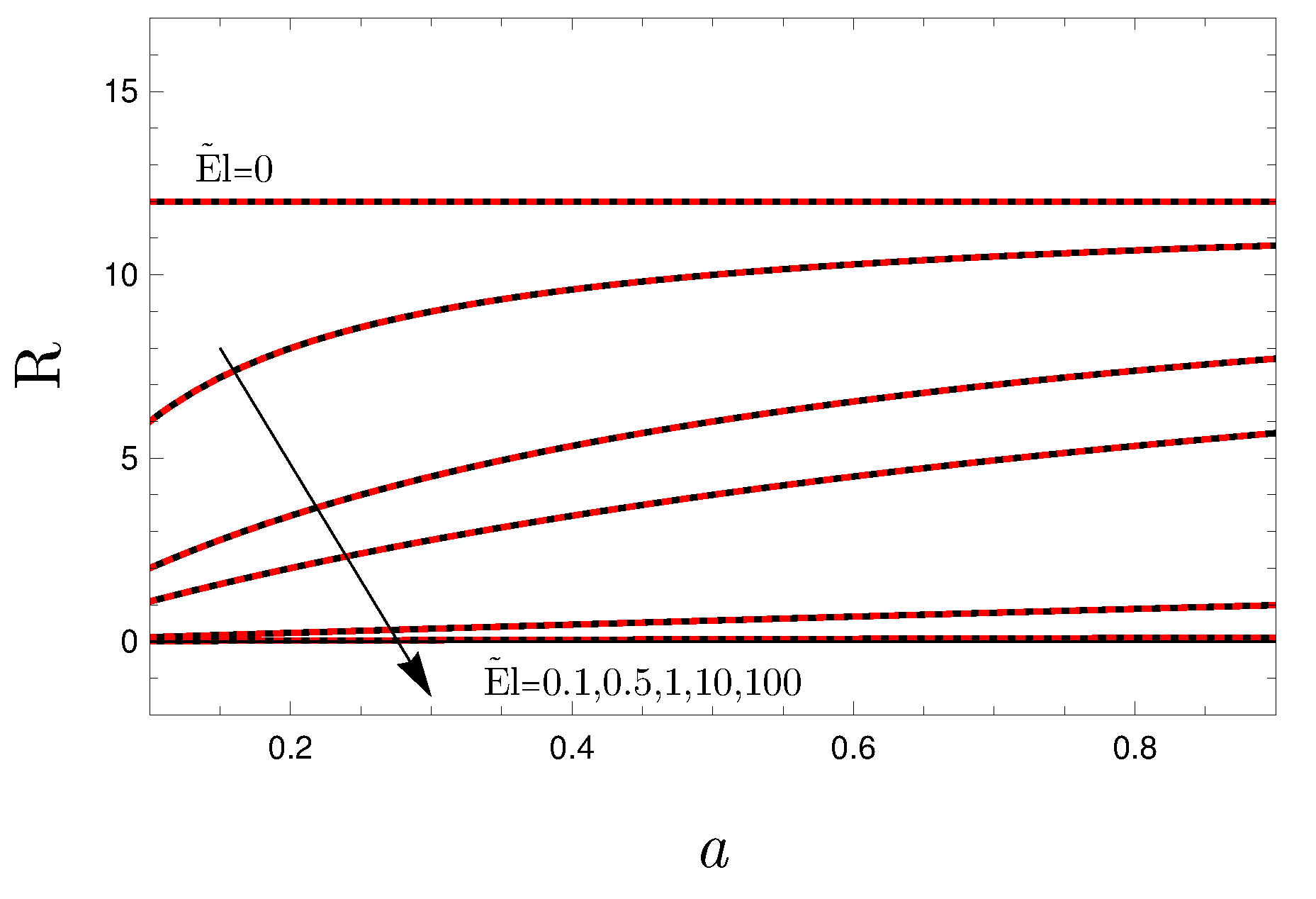
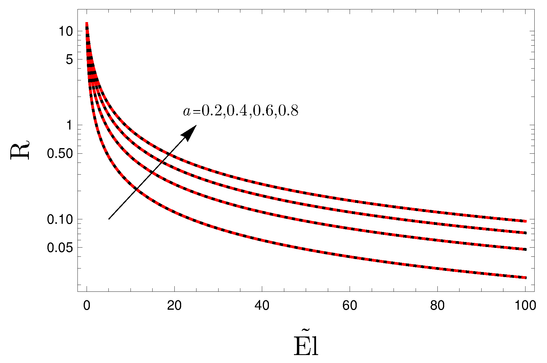
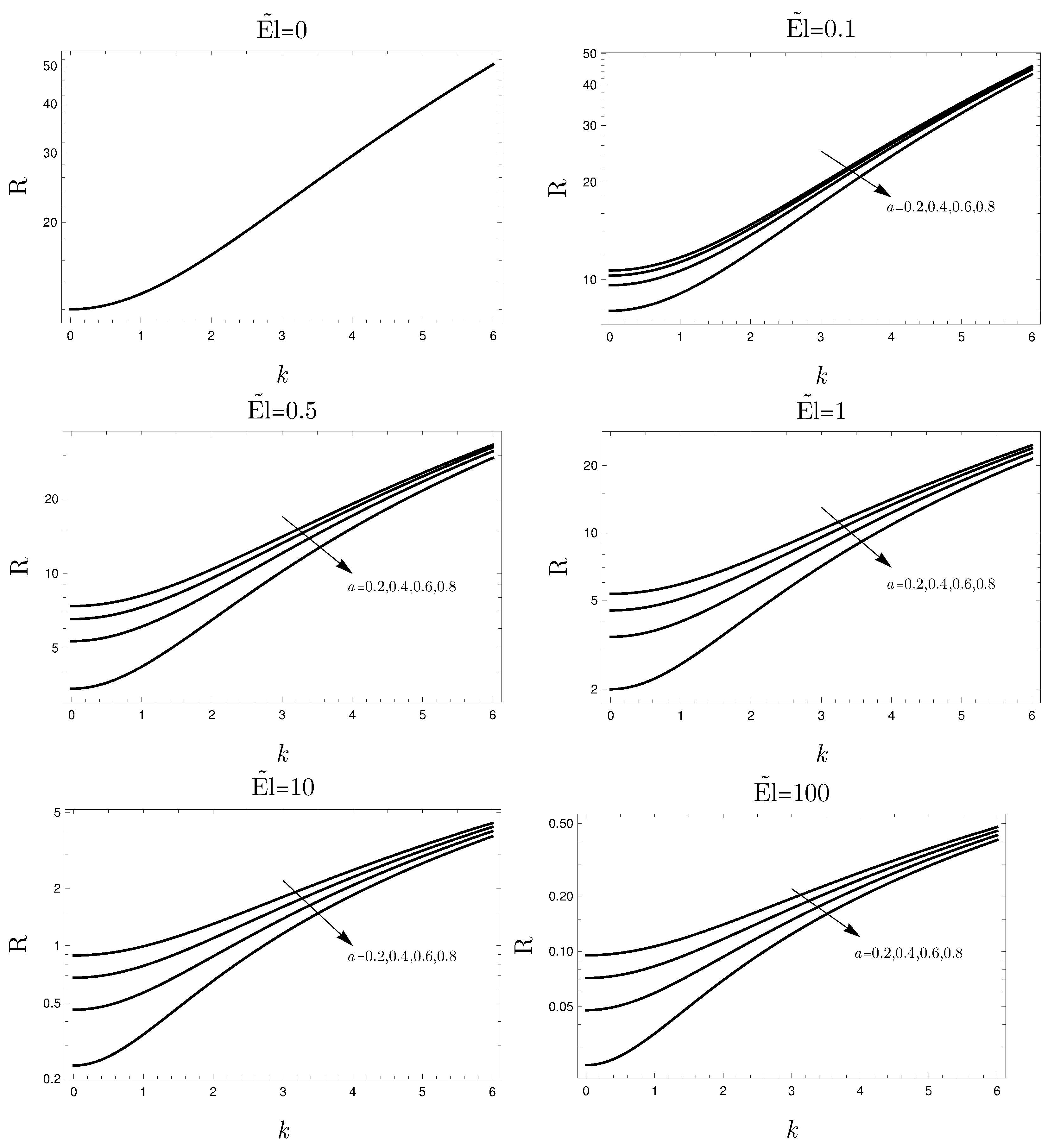
  • The non-Newtonian character of the fluid plays a destabilizing effect on the convective flow, namely an increasing value of the Ellis number yields a destabilization of the basic flow;
  • For El 0 , the Ellis index a does not affect the stability conditions and the results coincide with those for the limit of Newtonian fluid already available in the literature ( k c = 0 and R c = 12 );
  • For large values of the Ellis number, the power-law behavior is recovered. This means that the critical Rayleigh number tends to zero.

Author Contributions

All authors were invaluable to the creation of this paper. All authors have read and agreed to the published version of the manuscript.

Funding

This research was funded by Italian Ministry of Education, University and Research (MIUR) grant number PRIN 2017F7KZWS.

Data Availability Statement

The data is contained within the article.

Conflicts of Interest

The authors declare no conflict of interest.

References

  1. Nield, D.A.; Bejan, A. Convection in Porous Media, 5th ed.; Springer: New York, NY, USA, 2017. [Google Scholar]
  2. Shenoy, A. Non-Newtonian fluid heat transfer in porous media. In Advances in Heat Transfer; Elsevier: Amsterdam, The Netherlands, 1994; Volume 24, pp. 101–190. [Google Scholar]
  3. Nield, D.A. A note on the onset of convection in a layer of a porous medium saturated by a non-Newtonian nanofluid of power-law type. Transp. Porous Media 2011, 87, 121–123. [Google Scholar] [CrossRef]
  4. Nield, D.A. A further note on the onset of convection in a layer of a porous medium saturated by a non-Newtonian fluid of power-law type. Transp. Porous Media 2011, 88, 187–191. [Google Scholar] [CrossRef]
  5. Brandão, P.V.; Ouarzazi, M.N. Darcy–Carreau model and nonlinear natural convection for pseudoplastic and dilatant fluids in porous media. Transp. Porous Media 2021, 136, 521–539. [Google Scholar] [CrossRef]
  6. Brandão, P.; Ouarzazi, M.; Hirata, S.d.C.; Barletta, A. Darcy–Carreau–Yasuda rheological model and onset of inelastic non-Newtonian mixed convection in porous media. Phys. Fluids 2021, 33, 044111. [Google Scholar] [CrossRef]
  7. Celli, M.; Barletta, A.; Brandão, P.V. Rayleigh–Bénard instability of an Ellis fluid saturating a porous medium. Transp. Porous Media 2021, 138, 679–692. [Google Scholar] [CrossRef]
  8. Brandão, P.V.; Celli, M.; Barletta, A. Rayleigh–Bénard instability of an Ellis fluid saturated porous channel with an isoflux Boundary. Fluids 2021, 6, 450. [Google Scholar] [CrossRef]
  9. Savins, J.G. Non-Newtonian flow through porous media. Ind. Eng. Chem. 1969, 61, 18–47. [Google Scholar] [CrossRef]
  10. Horton, C.W.; Rogers, F.T. Convection currents in a porous medium. J. Appl. Phys. 1945, 16, 367–370. [Google Scholar] [CrossRef]
  11. Lapwood, E.R. Convection of a fluid in a porous medium. Proc. Camb. Philos. Soc. 1948, 44, 508–521. [Google Scholar] [CrossRef]
  12. Prats, M. The effect of horizontal fluid flow on thermally induced convection currents in porous mediums. J. Geophys. Res. 1966, 71, 4835–4838. [Google Scholar] [CrossRef]
  13. Sparrow, E.M.; Goldstein, R.J.; Jonsson, V.K. Thermal instability in a horizontal fluid layer: Effect of boundary conditions and non-linear temperature profile. J. Fluid Mech. 1964, 18, 513–528. [Google Scholar] [CrossRef]
  14. Park, H.; Sirovich, L. Hydrodynamic stability of Rayleigh-Bénard convection with constant heat flux boundary condition. Q. Appl. Math. 1991, 49, 313–332. [Google Scholar] [CrossRef]
  15. Nield, D.A. Onset of thermohaline convection in a porous medium. Water Resour. Res. 1968, 4, 553–560. [Google Scholar] [CrossRef]
  16. Jones, M.; Persichetti, J. Convective instability in packed beds with throughflow. AIChE J. 1986, 32, 1555–1557. [Google Scholar] [CrossRef]
  17. Sochi, T. Non-Newtonian flow in porous media. Polymer 2010, 51, 5007–5023. [Google Scholar] [CrossRef]
  18. Sadowski, T.J.; Bird, R.B. Non-Newtonian flow through porous media. I. Theoretical. Trans. Soc. Rheol. 1965, 9, 243–250. [Google Scholar] [CrossRef]
  19. Sadowski, T.J. Non-Newtonian Flow through Porous Media. Ph.D. Thesis, The University of Wisconsin-Madison, Madison, WI, USA, 1963. [Google Scholar]
  20. Wolfram, S. The Mathematica book (3rd ed.). Assem. Autom. 1999, 19, 77. [Google Scholar] [CrossRef]
Figure 1. Sketch of the porous layer heated from below and cooled from above by equal constant heat fluxes with horizontal throughflow.
Fluids 08 00054 g001
Figure 2. Neutral stability condition for different values of El and a ˜ .
Fluids 08 00054 g002
Figure 3. Comparison between asymptotic solution for k 0 (red dashed curves) and the neutral stability condition obtained numerically for k = 10 3 (black continuous curves); R versus a.
Fluids 08 00054 g003
Figure 4. Comparison between asymptotic solution for k 0 (red dashed curves) and the neutral stability condition obtained numerically for k = 10 3 (black solid curves); R versus El ˜ .
Fluids 08 00054 g004
Figure 5. Critical R as a function of the basic pressure gradient for different values of El for a = 0.2 and a = 0.8 .
Fluids 08 00054 g005
Table 1. Neutral stability values of R for small values of k for the Newtonian limit El 0 .
k R
0.1 12.0114
0.01 12.0001
0.001 12.0000
012
Table 2. Critical values of R .
El ˜ a = 0.8 a = 0.6 a = 0.4 a = 0.2
012121212
0.1 10.66666710.2857149.68
0.5 7.38461546.54545455.33333333.4285714
15.33333334.53.42857142
100.888888890.679245280.461538460.23529412
1000.0952380950.0715705770.0478087650.023952096
Disclaimer/Publisher’s Note: The statements, opinions and data contained in all publications are solely those of the individual author(s) and contributor(s) and not of MDPI and/or the editor(s). MDPI and/or the editor(s) disclaim responsibility for any injury to people or property resulting from any ideas, methods, instructions or products referred to in the content.

