Article

Simulating Flow in an Intestinal Peristaltic System: Combining In Vitro and In Silico Approaches

School of Chemical and Biomolecular Engineering, The University of Sydney, Sydney, NSW 2006, Australia
*
Author to whom correspondence should be addressed.
These authors contributed equally to this work.
Fluids 2023, 8(11), 298; https://doi.org/10.3390/fluids8110298
Submission received: 26 September 2023 / Revised: 5 November 2023 / Accepted: 7 November 2023 / Published: 10 November 2023
(This article belongs to the Special Issue Challenges and Directions in Fluid Structure Interaction)

Abstract

:
Transport and mixing in the gastric duct occur via peristaltic flow. In vivo data are hard to collect and require strict ethical approval. In contrast, both in vitro and in silico studies allow detailed investigation and can be constructed to answer specific questions. Therefore, the aim of this study was to design a new elastic thermoplastic polyurethane (TPU) intestine model and to compare the flow patterns observed experimentally with those predicted by a Fluid Structure Interaction (FSI) simulation. Here, we present complementary studies that allow feedback to improve both techniques and provide mutual validation. The experimental work provides direct measurement of mixing, and the simulation allows the experimental setup to be studied to determine the impacts of various parameters. We conclude by highlighting the utility of this approach.

1. Introduction

Studying the digestion process has been led by the demand for healthier eating all around the world. In vivo studies of food digestion are very complex, expensive, and time-consuming and require very careful ethical consideration [1]. In vitro digestion models are desirable alternative methods to simulate the process of human digestion [2]. To represent the digestion of foods in the human digestive system, a dynamic process is required. The digestive process is affected significantly by the mixing and flow patterns in the human gut [3].
Construction of such an experiment requires the use of a flexible transparent tube. Thermoplastic polyurethane (TPU) has mechanical properties that allow high elongation and is an elastomer [4]. Polyurethane has been applied in the medical field, such as in artificial heart valves [5,6]. It can be deformed in a controlled way to generate peristaltic flow.
Computational Fluid Dynamics (CFD) can be used to study flow and mixing in the digestion process. Computational modeling can help to understand the complex behavior inside the human intestine. CFD can simulate the motility and geometry of the intestinal system. The flow patterns in the digestion process have been examined by some developed CFD models to study fundamental mechanisms, including 2D (two-dimensional) CFD [7,8,9] and 3D (three-dimensional) CFD [10,11,12,13] models. The behavior of Newtonian fluids has been studied by Ferrua and Singh [13] for gastric flow by a CFD simulation, allowing the prediction and visualization of the flow patterns, shear stresses, and shear rates. Fluid–structure interaction (FSI) can be used to study the interaction between a movable structure and the internal fluid flow. A combination of the Navier–Stokes and elastic wave equations can be used to simulate the fluid flow inside the duodenum driven by a peristaltic wave.
The object of this research was to produce an artificial human intestine model. The system has been designed to mimic natural peristalsis. The elastic TPU intestine model was prepared using 3D printing technology. The advantages of using this technology are that models with specific sizes and scales are readily designed and built. The mechanical property of this TPU intestine model has been analyzed. With the help of cameras and computer analysis programs, flow patterns within the intestine model have been obtained and analyzed using fluorescein dye. Furthermore, the experimental results from the physical model have been compared with FSI simulations.
Section 2 provides detailed descriptions of the development of the in vitro and in silico models. The results and discussion are presented in Section 3, and the conclusions are given in Section 4.

2. Materials and Methods

In this section, both the experimental and simulation setups are presented in detail.

2.1. The In Vitro Model

2.1.1. Materials

TPU was used to construct the in vitro model by 3D printing technology. In the intestine model system, a 3D-printed mold (TPU), 3D-printed clamps and supporting rings (PLA), lighting box, tubes, valves, gear pumps, metal stands’ syringes, controlling box (for gear pumps), cameras (Logitech C930e Advanced HD Webcam, Lausanne, Switzerland), computer (software, LabView, Version 2020, National Instruments, Tokyo, Japan), and lighting system (LED light strip) were required to set up the system. Fluorescein dye was used in the flow pattern tests.

2.1.2. Manufacturing the TPU Model

TPU is a rubber-like material that can be printed with modern 3D printers (CammPro 3D Print, using fused deposition and a 1.2 mm nozzle). The length of the tube was about 240 mm. Due to the limitations of the 3D printer used to create the model, the intestine model was separated into two parts, as shown in Figure 1. These parts were connected using an overlap section. The flexible TPU tube was waterproofed by adding a transparent silicon sealant outside the tube. Figure S1 shows the scales of the different parts of the intestine model. Jacobs et al. [14] graded the small bowel distension into four sections, including non-dilated, mildly, moderately, and severely dilated, with the corresponding sizes being less than 25 mm, 25–29 mm, 30–40 mm, and larger than 40 mm. Therefore, the diameter of the in vitro intestine model was designed to be 40 mm. To enhance the mixing process and transport phenomena, the in vitro model was flexible. Therefore, it can be manipulated to simulate the physical behavior of the real intestine.

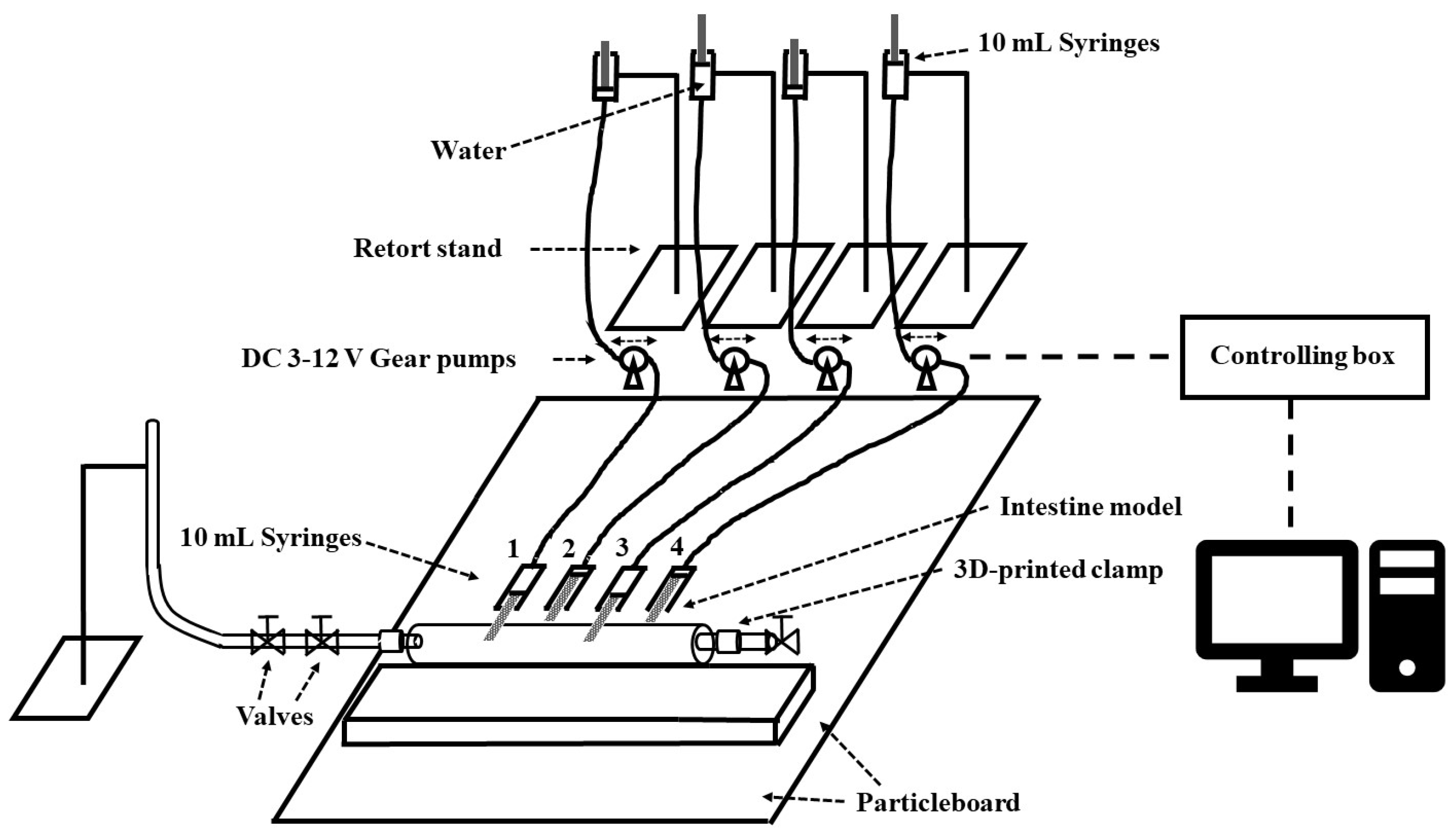
2.1.3. Arrangement of the In Vitro Intestine System

Gear pumps and syringes were set up to create an actuator system that controlled the movement of the intestine model. Coding the control profile enabled the control box to manipulate frequencies and intensities by compressing the intestine model. The 3D-printed clamps were used to fix the location of the hydrogel intestine model.
To research the flow pattern in an in vitro TPU intestine model, four actuators were developed in combination with a computer control system. The inflation and deflation of the in vitro intestine model was produced using a linear actuator system. Figure 2 shows the outline of the complete physical system. The linear actuators consisted of syringes, plastic tubing, gear pumps, and water. The movement of the syringes was controlled by the gear pumps, which were operated by the computer through an interface. The amplitude and frequency of the syringes were controlled automatically, and, furthermore, the movements of the in vitro intestine model were controlled. The experiments were operated at room temperature (~20 °C). The peristaltic flow was generated by squeezing the tube with actuators, as shown in Figure 3.

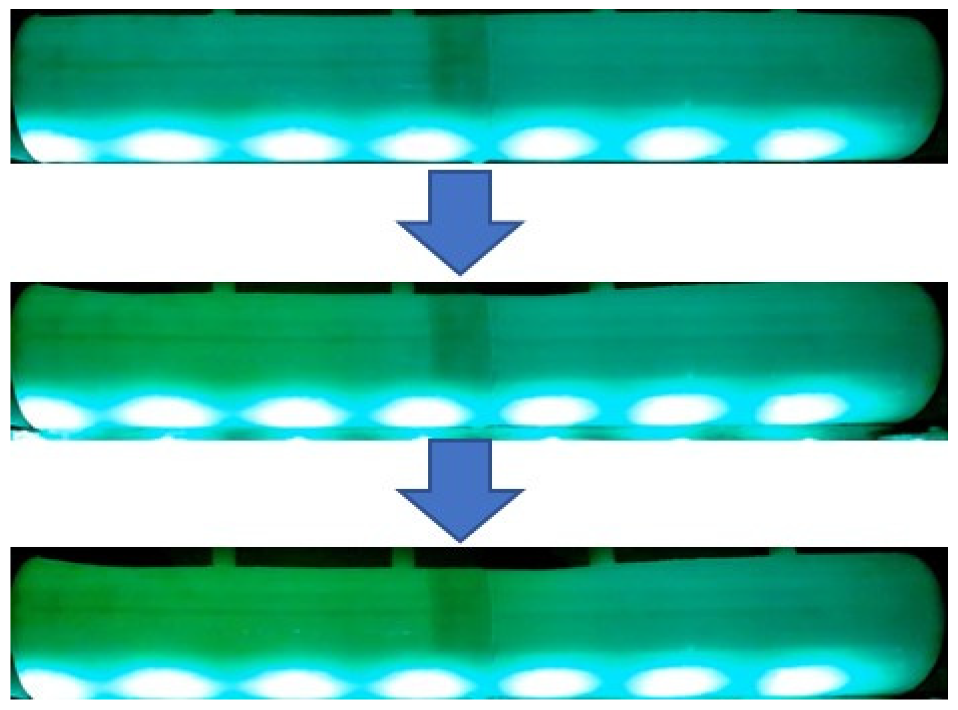
2.1.4. Flow Visualization Tests

The TPU intestine model was used to study the flow patterns of the fluorescein dye (100 g fluorescein (free acid), Sigma-Aldrich (Melbourne, VIC, Australia)). The dye was diluted in water to a concentration of 0.3 g/L. The diluted dye was injected into the TPU intestine model using a syringe, with 6.5 mL of dye solution being injected for tests. The model was tested with various control profiles, as shown in Table S1.

2.1.5. Color Analysis

The flow pattern in the intestine model was recorded as videos and images during flow visualization studies and were analyzed by color analysis using MATLAB, version 9.13.0.2166757 (R2022b) Update 4. For the MATLAB analysis, multiple regions of 10 × 10 pixels were used to assess the L , a , and b values (color parameters) for the collected photos according to the CIELAB sphere [15]. A calibration process was introduced to translate the Lab values to dye concentrations.

2.1.6. Tensile Tester

A universal mechanical tester (Shimadzu EZ-L, shown in Figure S2, Kyoto, Japan) was used to perform mechanical tests in air at room temperature for assessing the stiffness of the models, specifically the Young’s moduli.

2.2. The In Silico Model

Fluid Structure Interaction (FSI) analysis in this study was performed using Ansys System Coupling 2022R1. Fluid dynamics analysis was conducted using Ansys Fluent, version 2022R1, which used the finite volume method (FVM). The transient structural analysis was developed using Ansys Mechanical, version 2022R1, using the finite element method (FEM). During the simulation, the Fluent and Mechanical solvers were run simultaneously, with data at the interface between the models being transferred via System Coupling 2022R1.

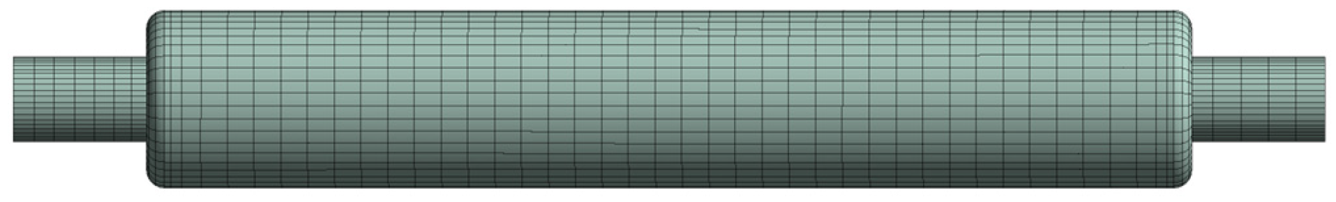
2.2.1. The Fluid Domain Model

Ansys SpaceClaim was used to construct the fluid domain, containing the main mixing chamber and a riser tube. The riser tube contained a vertical section and a 90° bend connected to the chamber. The smaller inner tube inside the riser tube was used to inject the dye into the system. The geometry also included the supports used to hold the inner tube in place. The geometry is shown in Figure 4.
The Ansys Fluent Watertight Geometry meshing template was used to generate the mesh in the fluid region (see Figure 5). The mesh was made from tetrahedral cells with inflation at the walls and comprised 930,000 cells with a minimum orthogonal quality of 0.25. The mesh sizing was chosen based on test cases conducted to ensure adequate flow resolution.
The transient, pressure-based solver was used to simulate turbulent flow. The Reynolds number was around 3000, which means it was a turbulent flow, but the Reynolds number was low, lying within the laminar–turbulent transition regime. The SST k-ω model [16] was used to simulate the turbulent flow, as it behaved well even at low Reynolds numbers because of its ability to integrate to the wall.
Conservation equations for mass, momentum, and species transport were solved, together with a Tait Equation of State (EOS) for water. Compressible flow was solved so that artificial compressibility could be used to improve simulation stability at the initial coupling stages, as observed by La Spina [17]. This was found to be especially important here when high pressures were developed during convergence, as high loads were transferred at the start of each timestep.
The compressible liquid had a reference density ( ρ 0 ) of 1000 kg/m3, a reference bulk modulus ( K ) of 100 kPa, a density exponent ( n ) of 1, and a density ratio limit of 0.9 ( ρ r , m i n ) to 1.1 ( ρ r , m a x ), which meant that the density of the liquid ( ρ ) could vary from 990 to 1100 kg/m3. The density variation was found to be less than 1% (discussed later) and therefore the fluid flow was very close to incompressible.
The species transport model was used to simulate the mixing between the water and dye solution. Water and dye were assumed to have the same properties. The diffusion coefficient of fluorescein in water is 3.4–5.0 × 10⁻¹⁰ m2/s [18]. The effect of diffusion was therefore small or negligible during the experiments. In the simulation, the species diffusion coefficient ( D ) was set to 4.2 × 10⁻¹⁰ m2/s, which was the mid valve in the range. All walls were set to have no slip and no flux of dye. The top boundary of the vertical tube that was open to the atmosphere was set as pressure opening, having a static gauge pressure of 0 Pa. All the other boundaries were set as non-slip walls. To set up the initial condition, the fluid domain was filled with water. Then, a small region was patched with the dye, as shown in Figure 6. The region in blue color represents water, whereas the region in red color represents dye. The initial dye concentration was set to 0.3 g/L, with a total dye mass of 1.9 mg.
A dynamic mesh model was applied in the system-coupling zone (the main chamber in Figure 4a). The diffusion-based smoothing method was chosen so that the boundary motion could diffuse uniformly throughout the interior mesh [19]. The deforming boundary cells were remeshed when the cell skewness exceeded 0.9. This approach has been previously validated for peristaltic flow [20].
To record the dye concentration, the five locations along the centerline of the tube used in the experiments were selected. The TPU material used was not fully transparent, and the clear color observation range was tested to be 10 mm from the surface. Therefore, in the simulation, a line was drawn into the flow from each visualization point. The average dye concentration along the entire line and 10 mm from the surface, as shown in Figure 7, was recorded every 0.1 s to accommodate the uncertainty in the experimental observation window.
The Pressure-Implicit with Splitting of Operators (PISO) pressure-velocity coupling scheme and the first-order implicit transient formulation were used. This is a pressure-based flow solver with variable density and works in the same way as an incompressible flow solver. Gradients were determined using the least-squares cell-based option, and the pressure was determined using the second-order method. The first-order upwind scheme was used for the density and turbulence variables. The second-order upwind scheme was used for the momentum equations and the dye concentration. Converged solutions were achieved when globally scaled residual values for the continuity, x, y, and z velocities, turbulence quantities, and dye mass fraction were below 10−3. The maximum iteration number for each coupling step was set to 50, whereas 20 were usually needed for convergence.

2.2.2. The Structural Domain Model

Ansys SpaceClaim was used to construct the structural domain, composed of three parts: the main body, where the peristaltic motion occurred; four pistons that were used to compress the main body; and the supporting structure. The structural geometry is shown in Figure 8. The main body (colored in green) was deformable. Both the pistons (colored in purple) and the supporting body (colored in pink) were treated as rigid bodies.
TPU was used to construct the deforming body of the model. Based on the results from mechanical testing, the Young’s modulus and Poisson’s ratio of the material were set to 15.5 MPa and 0.45, respectively.
The main body of the system could be easily deformed by the pistons due to the elasticity of the TPU material. To hold the main body in place, it was crucial to define the connections between the main body and its nearby bodies properly. The connections between the main body and the pistons were defined as frictional, with a frictional coefficient of 0, meaning that the contact surfaces could slide and separate without resistance. To hold the main body in place, the connections between the main body and the supporting bodies were set to be frictional, with a frictional coefficient of 0.05. Both ends of the deforming geometry were constrained to avoid movement outside of the supporting body. The augmented Lagrange and nodal detection methods were used for all contacts. The normal stiffness factor was chosen to be 0.01 N / m to ease the convergence difficulties. These connections are summarized in Figure 9.
Prior to mesh construction, virtual topology and body splitting were utilized so that the solid could be split into hexahedral elements, which are preferred over tetrahedral elements in Finite Element Analysis (FEA). The final mesh used comprised 4100 hexahedral elements having a maximum skewness of 0.87 (see Figure 10).
Remote displacements were applied on the pistons to simulate their movement. The compression distance of each piston was extracted from the experimental data and used in the simulation. The Direct solver was used with large displacements enabled to capture the material deformation. Validation was performed to ensure that the model setup and mesh captured the propagation of elastic waves correctly [21].

2.2.3. System Coupling

Ansys System Coupling, version 2022R1, was used to couple the fluid and structure interfaces. The simulation started with the motion of the pistons acting on the deformable body. A timestep size of 0.1 s was found to be suitable. The simulation was run for 292 steps, giving a total simulation time of 29.2 s. The maximum iteration number for each time step was set to 10, whereas usually 6 were needed for convergence. Quasi-Newton stabilization was activated for data transfer, with an initial relaxation factor of 0.05 and one retained timestep in the Quasi-Newton history. Data transfers at the interface converged when the globally scaled RMS (Root Mean Square) the residual values were below 0.01.
Twelve cores of a computer with an Intel(R) Xeon Bronze 3204 @1.90 GHz processor and 64 GB RAM were used to run the model. Ansys Fluent and Ansys Mechanical were allocated five and seven cores, respectively. An NVIDIA Quadro RTX 6000 (Santa Clara, CA, USA) graphic card (GPU) was utilized to accelerate the structural simulation process. The total simulation time for the FSI analysis was 88 h running on the above machine, with Fluent using 38 h and Mechanical using 50 h.

3. Results and Discussion

Firstly, results from the physical experiments are presented to show flow behavior observed in the in vitro model, as well as the flow patterns. Then, results from simulations are presented to show the overall flow and mechanical behavior of the system. A comparison of the measured and simulated dye concentrations is also provided.

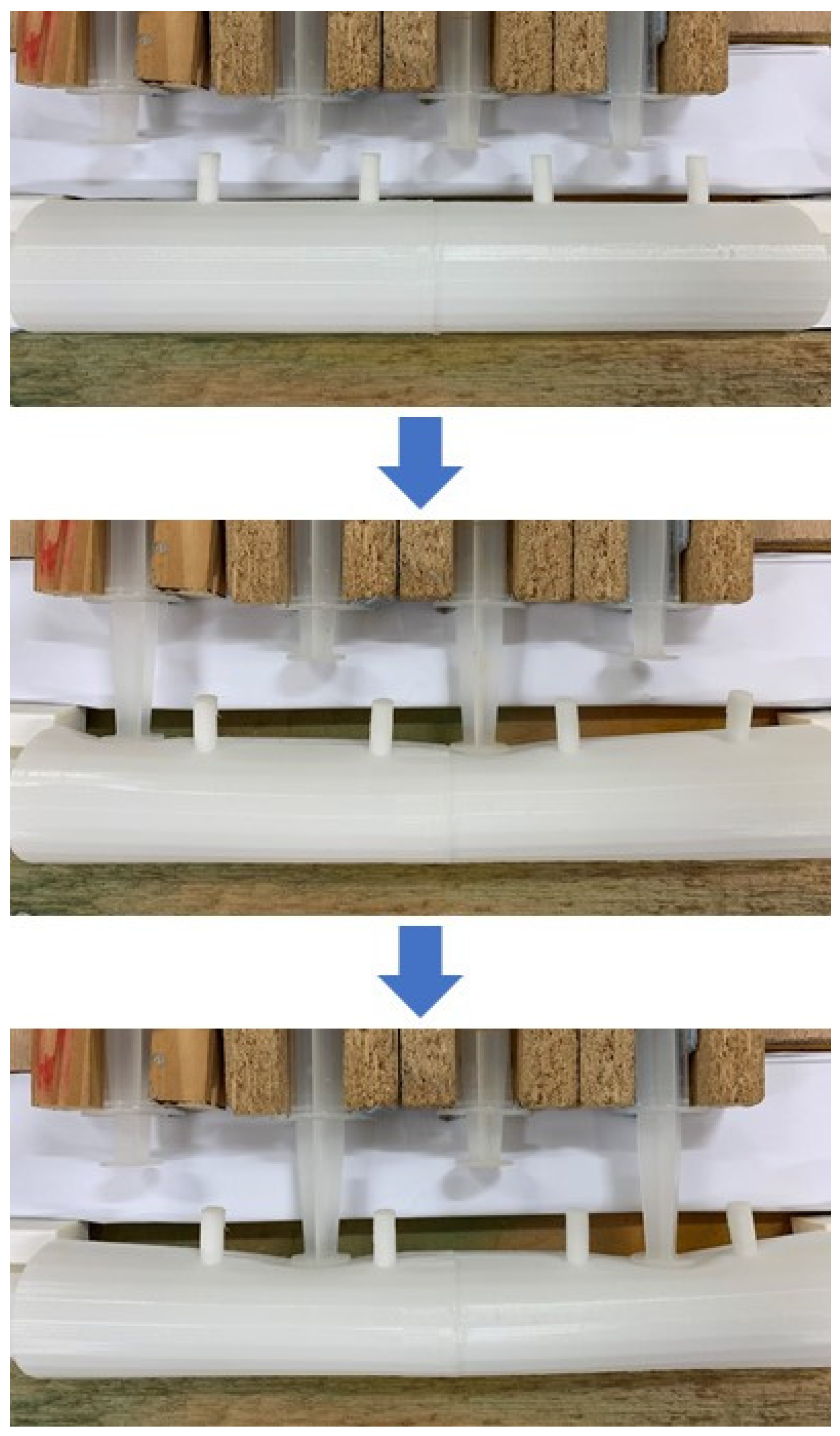
3.1. Physical Features of the Intestine Model

The fused deposition modeling (FDM) method was used to 3D print the intestine model with TPU. This is a material extrusion method for additive manufacturing. Three-dimensional models were created by extruding the material through a nozzle and joining it together. The melted material was deposited on the platform in layers, and these layers merged with each other to build the 3D models. The layer height was approximately 100 microns. Different sections of the TPU intestine model were measured using a tensile tester to study the mechanical properties, as shown in Figure S2. The values of Young’s modulus were found to vary from 12.9 MPa to 22.1 MPa. The reason for this variation is that the 3D printing process affects the stiffness of the model. The interfacial adhesion between the layers for the 3D process is variable for different structures of the model. Similar or closer locations have closer Young’s moduli, such as Samples 5, 6, 7, and 8. The locations with different shapes have Young’s moduli with larger differences, such as Samples 1, 2, and 9.

3.2. Experimental Results

The TPU intestine model was not totally transparent, so fluorescein dye was used to study the flow pattern inside the physical model. The dye movement process was recorded for analysis. The video was recorded in the dark with only a green LED light strip to reduce the impacts of the ambient lighting sources. Figure 11 shows the flow pattern when some fluorescein dye was inside the TPU model.
To analyze the dye flow, the video of fluorescein dye movement was changed into a series of pictures with small time intervals between frames (a frame-grabbing process). Two software packages were used to carry out this process: Premiere Pro and MATLAB. For each test, five sampling positions were studied with LAB values. By converting the LAB values to concentrations using a concentration calibration curve (from known concentrations), the concentration of each sampling position could be estimated as a function of time.
The four actuators continuously pushed the TPU intestine model in the rhythm described in Table S1. The largest displacement of the input was close to 18 mm, as shown in Figure 12a. Figure 12 shows the experimental inputs (displacement versus time) and outputs (concentration versus time). The displacements drove the physical model outputs and the simulation outputs. For Figure 12a,b, the time zero is the same for both curves, so the initial time is synchronized. A significant correlation between the inputs and the outputs is that pistons moved outwards (away from the model) at around 3 s in Figure 12a, and, at the same time, the dye was sucked into the model, which led to concentrations at Positions 1, 2, and 3 suddenly increasing, as shown in Figure 12b. When the dye was injected into the model, the concentration increased rapidly initially. With the continuous squeezing process, part of the dye moved backward, so there was a decrease in the dye concentration in the fluid flowing forward (the color of the intestine model became lighter because the dye was pushed backward). Dye concentrations at Points 1 to 3 increased quickly to 0.015 g/L at 30 s, whereas concentrations at Points 4 and 5 increased very slowly.
The flow experiments were repeated. To study the extent of repeatability for the flow visualization tests, the RMS errors were calculated for different operating conditions using
x R M S = 1 n ( ( x 1 T e s t 1 x 1 T e s t 2 ) 2 + ( x 2 T e s t 1 x 2 T e s t 2 ) 2 + + ( x n T e s t 1 x n T e s t 2 ) 2 )
where x R M S is a root mean square error, x n T e s t 1 and x n T e s t 2 are the values of the concentrations in Tests 1 and 2, respectively. The results, presented in Table 1, show the variation between the tests to be small compared with the mean values.

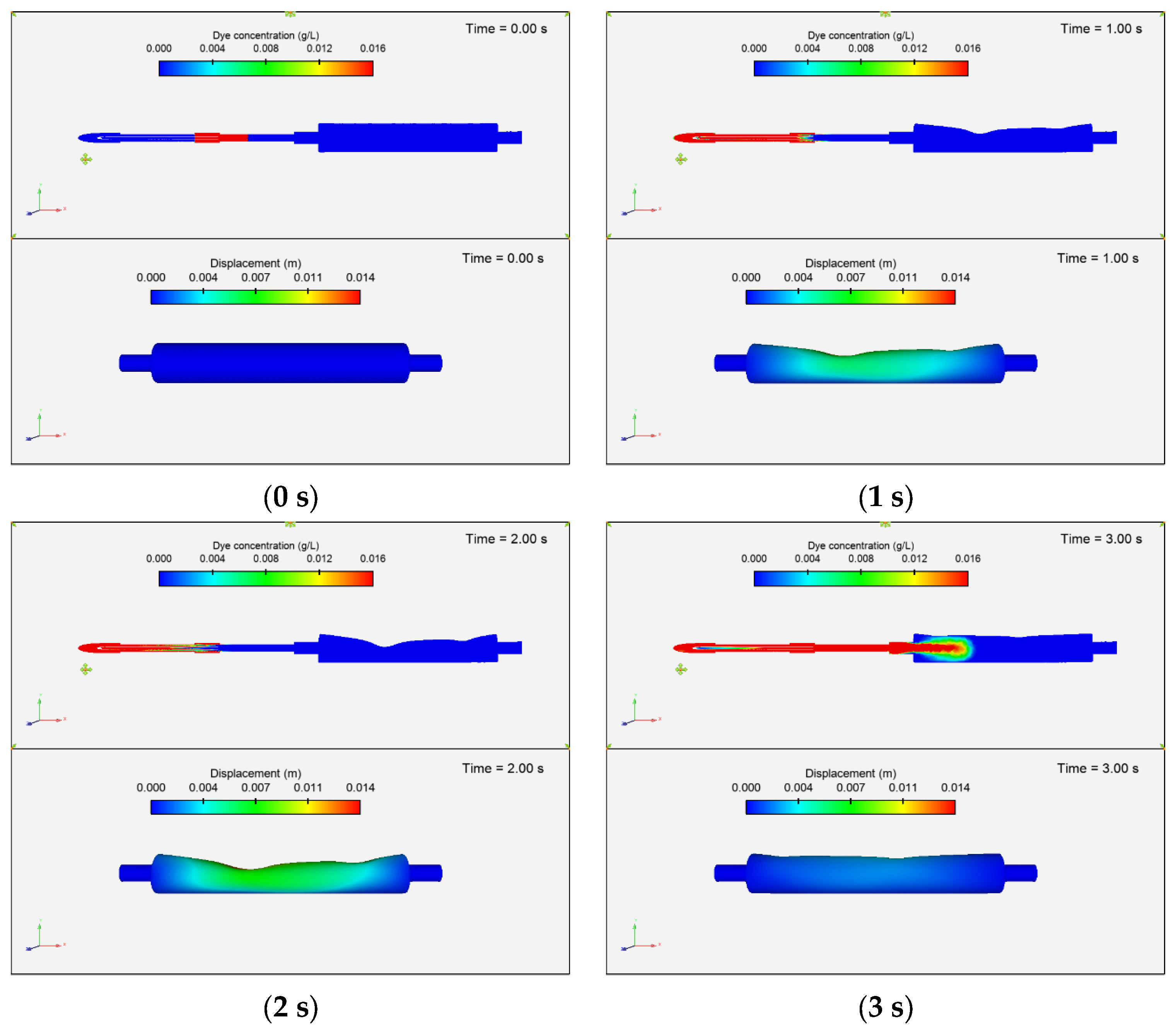
3.3. Simulation Results

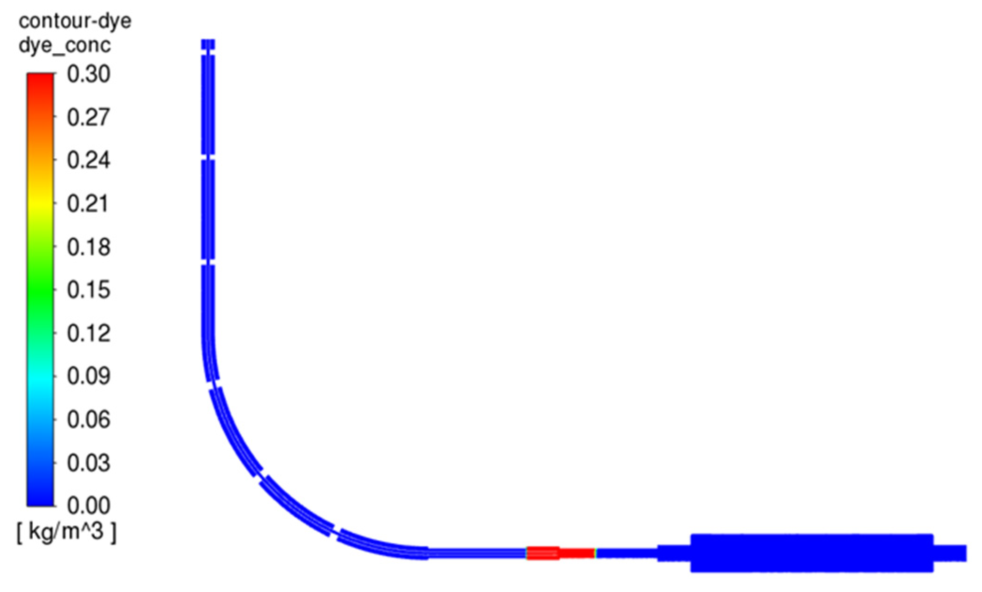
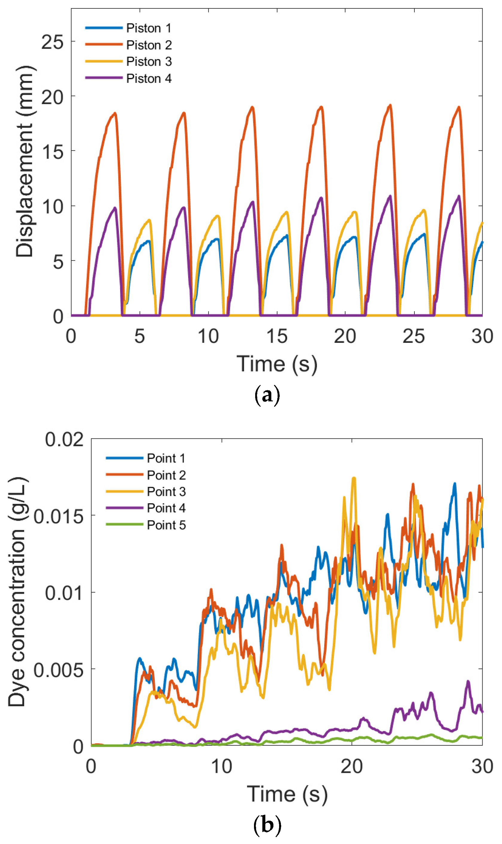
3.3.1. Dye Concentration and Chamber Displacement

The dye flow in the fluid domain and the deformation of the main chamber in the first cycle (0–5.1 s) are shown every 1 s in Figure 13 and Videos S1 and S2. The top images in Figure 13 present the dye flows, and the bottom images show the deformations of the deformable body. From 0 to 2 s, pistons 2 and 4 were compressing the tube, and the dye started to spread out along the riser tube. From 2 to 2.6 s, pistons 2 and 4 began to lift, causing fluid to flow back into the main chamber. After the movement of pistons 1 and 3 from 2.6 to 5.1 s, more dye spread out in the chamber.
After each cycle, more dye was pulled into the main chamber due to suction caused by decompression. Figure 14 shows the dye concentration at the end of each cycle. At the end of the simulation (29 s), the dye had spread to the middle of the main chamber.

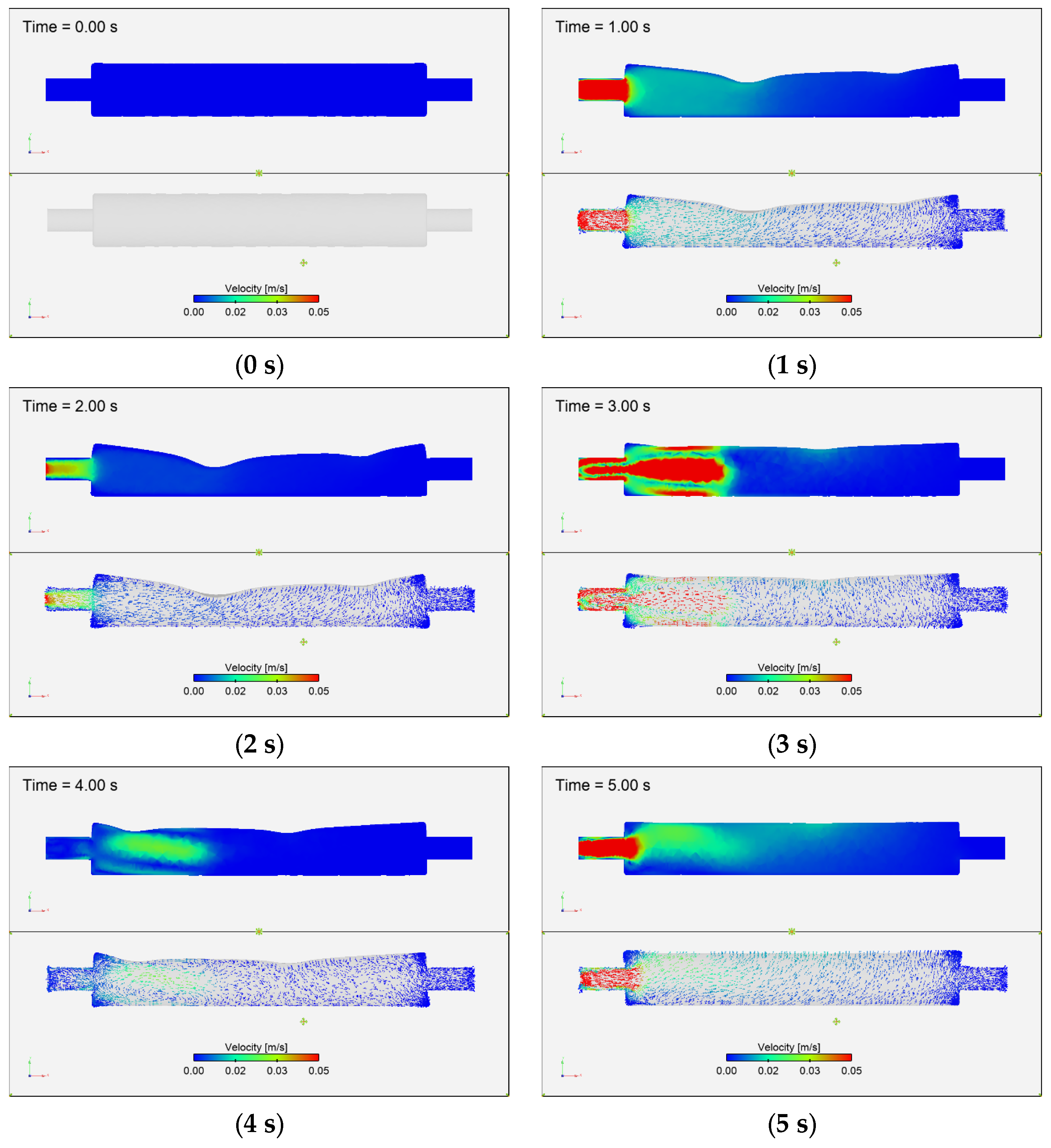
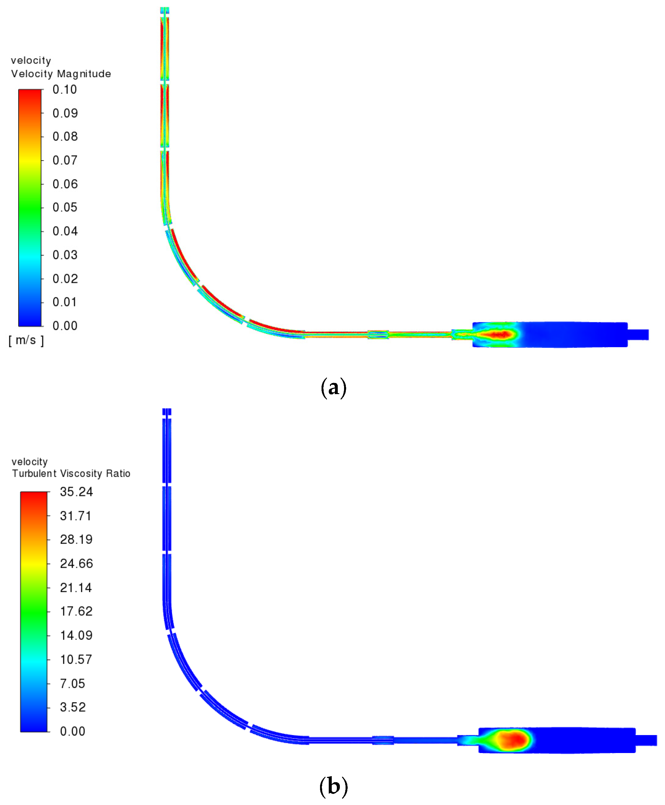
3.3.2. Fluid Velocity Field

Figure 15 shows the fluid velocity magnitude field in the first cycle. The top images show velocity contour plots, and the bottom images present the velocity vectors. The highest speed inside the chamber was around 0.1 m/s at 3 s when the pistons were lifted, and flow returned into the chamber. Most of the fluid motion occurred in the first half of the chamber and did not reach the other end.

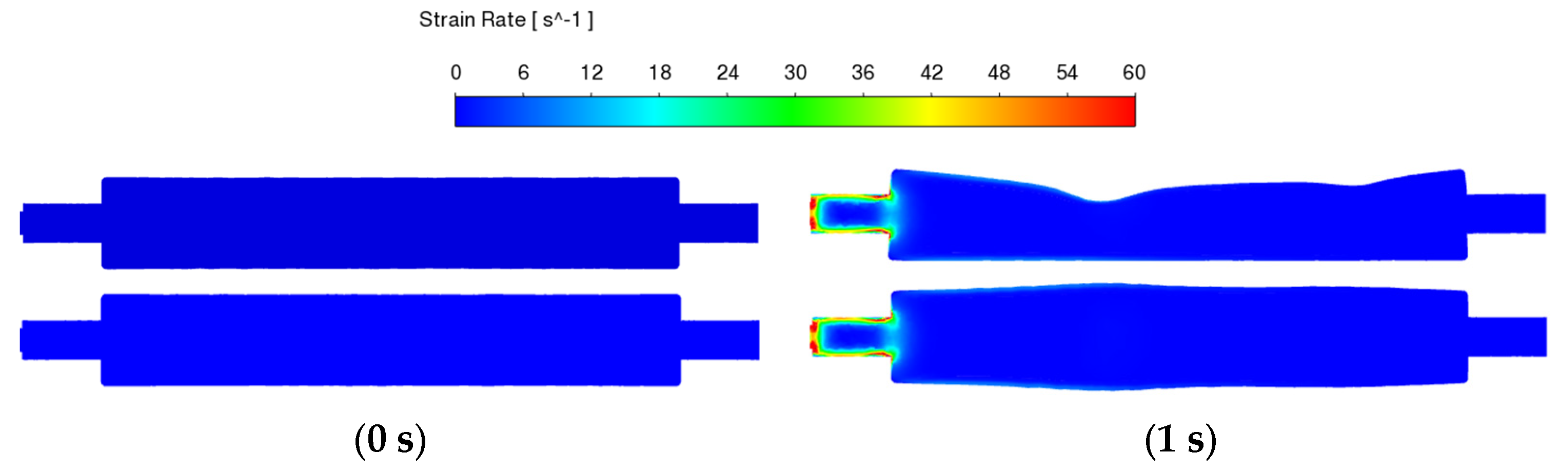
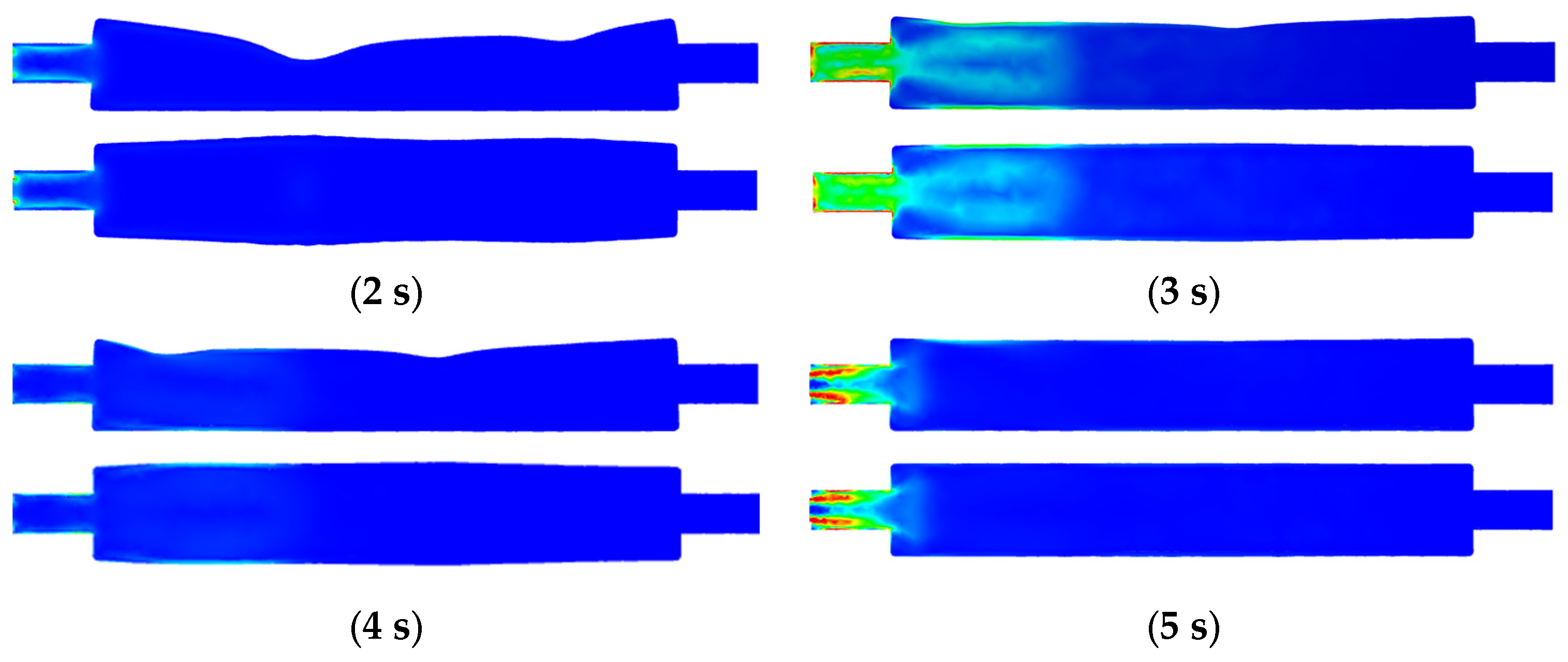
3.3.3. Fluid Strain Rate Changes

Strain rate is closely related to food disintegration and dissolution in the digestion process. It describes the velocity gradients in the fluid flow. The fluid strain rate contour plots for the first cycle are presented in Figure 16. The top images show the side view, and the bottom images show the contact surfaces where the pistons were compressing. The strain rate inside the flow ranged from 0 to 60 s−1, which matched the strain rates in different digestion systems [22]. The red color in the figure represents values that are 60 s−1) or above. The values near the wall at the entry were much higher and reached up to 380 s−1).

3.3.4. Reynolds Number and Turbulence Behavior in the Flow Regime

The Reynolds numbers were different in the riser tube and the main chamber, and the maximum speed at each part was observed at different times. The peak flow speed in the riser tube was around 0.25 m/s at 1 s, when the compression distances of the pistons were the largest, as shown in Figure 17a. With a riser tube diameter of 13 mm, the Reynolds number was estimated to be 3250 for the riser tube at 1 s. Only a small effect of turbulence was observed at this time point, as the turbulent viscosity ratio in the fluid was less than 3, as shown in Figure 17b.
The peak flow speed in the main chamber was around 0.1 m/s at 3 s when the pistons were lifted, and flow was returning into the chamber, as shown in Figure 18a. With a chamber diameter of 37 mm, the Reynolds number was 2960 at the main chamber at 3 s. The turbulent viscosity ratio in the system was much higher at this time point, as shown in Figure 18b. Therefore, the fluid flow was turbulent, which justified why the SST k-ω model, which is physically consistent at lower Reynolds numbers, was used to solve the flow.
The Reynolds numbers reported in other studies (including in vivo, in vitro, and in silico) varied from 3 [9] to 4688 [23], and our value was within the range. The Reynolds numbers in the gastric models depend on several factors, with the two most important factors being the form and magnitude of the external forces and the fluid viscosities. The external forces in the in vitro systems are difficult to measure, as the devices take different forms; some used a peristaltic system, and some used beaker systems [22]. The viscosity used in in vitro studies is usually within the range of 1 mPa·s to 50 Pa·s [22], and the values are 1 mPa·s to 10 Pa·s [11] in silico. However, the apparent viscosity of carbohydrate-based meals during digestion measured in vivo is 10–1500 Pa·s [24], which is orders of magnitude higher. In this study, water with a viscosity of 1 mPa·s was used, and therefore the calculated Reynolds number was relatively higher than values reported in some other studies.

3.3.5. Fluid Density Changes in the Simulation

A weakly compressible liquid was used to solve the fluid flow to help with convergence. The changes in fluid density at 3 s and 5 s when compression and decompression happen can be seen in Figure 19. The density variation was less than 1%, and therefore the fluid flow was very close to incompressible.

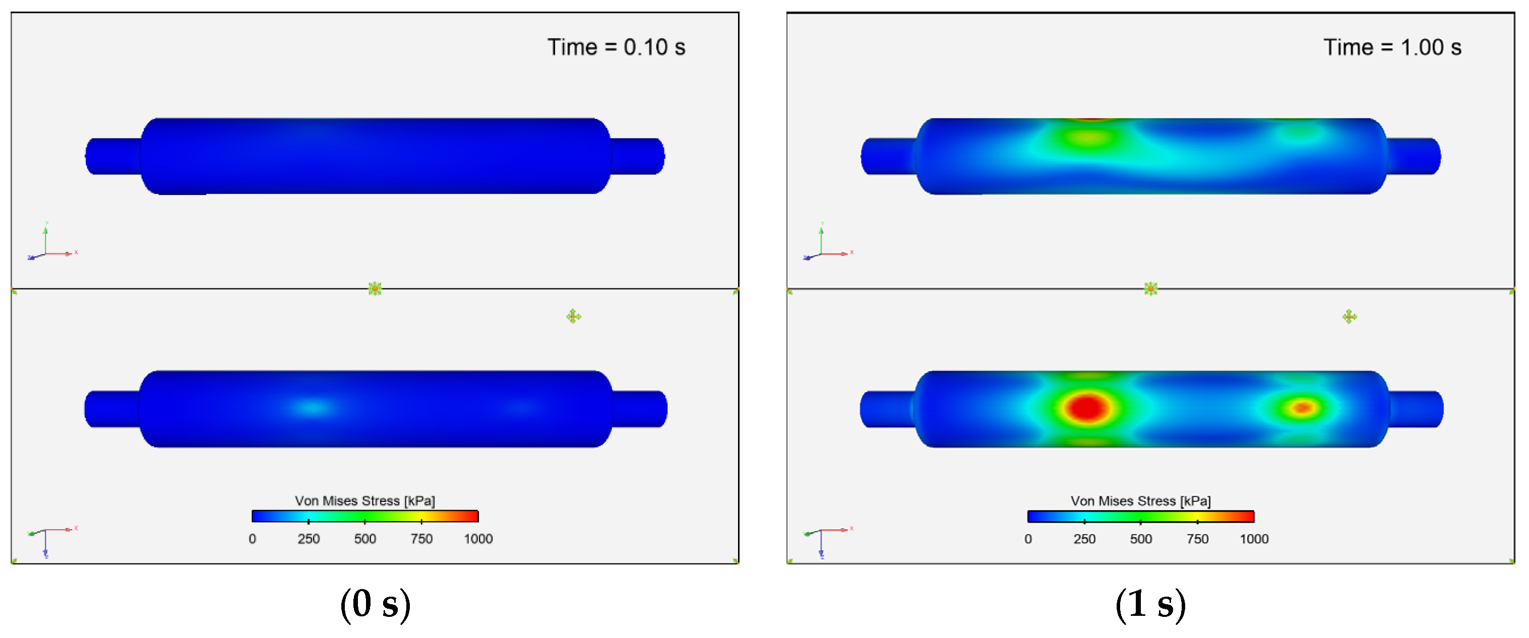
3.3.6. Von Mises Stress Distribution

The von Mises stress in the deforming structure is shown in Figure 20 at every second for the first cycle. The top images show the side view, and the bottom images show the view of the contact surfaces. The maximum von Mises stress in the deforming structure was 1.17 MPa at 2.1 s.

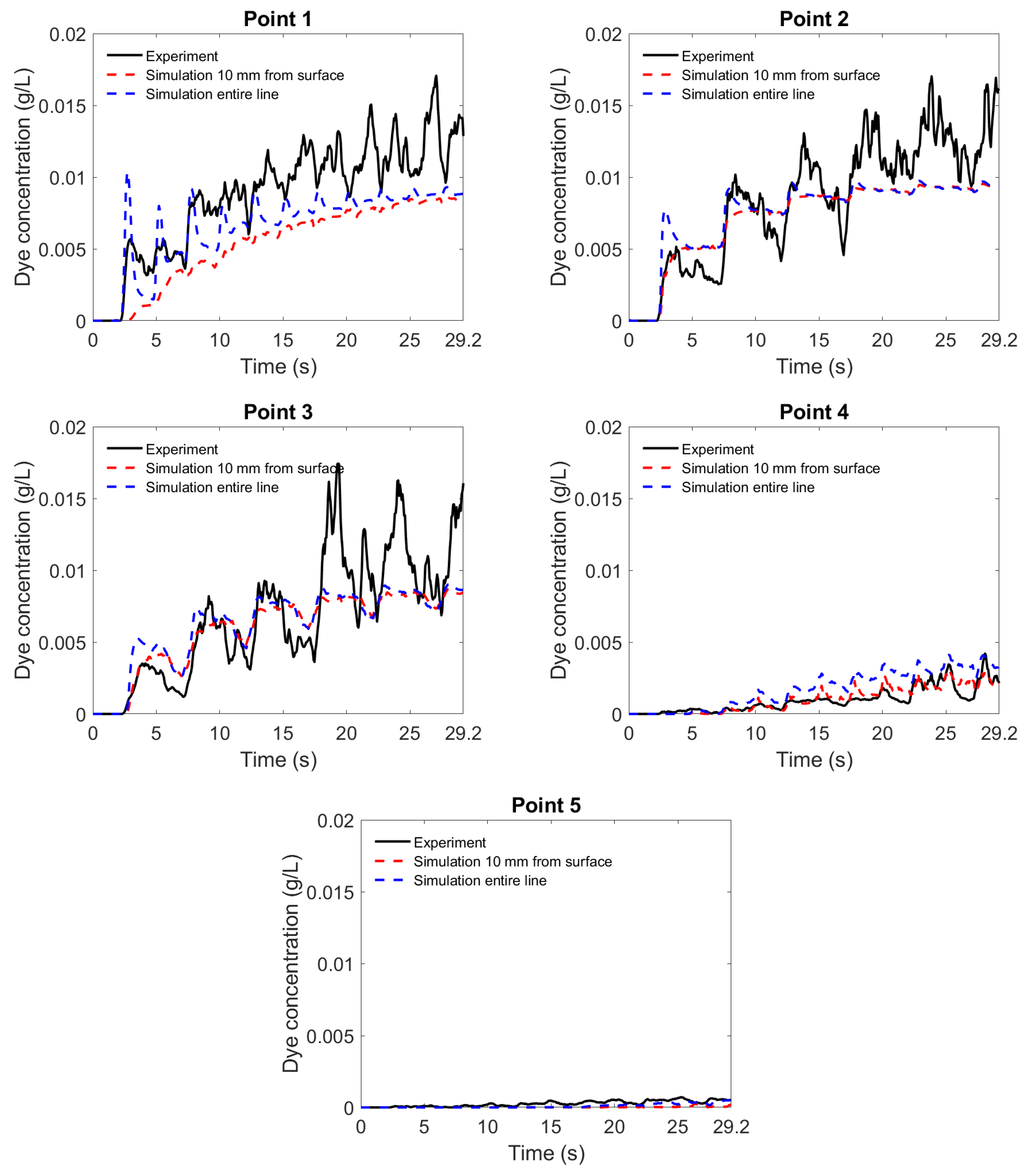
3.4. Comparison of Flow and Mixing Data between Experiment and Simulation

The dye concentration at each location is compared between the experiment and simulation in Figure 21. At 2.3 s, the dye entered the main chamber, and its concentration was observed to rise rapidly in both the experiment and simulation, this being especially evident at points 1, 2, and 3. From 2.4 to 2.8 s, pistons 2 and 4 were lifting and causing expansion in the chamber. The dye flowed into the chamber and reached the first peaks at around 2.7 s. When pistons 1 and 3 compressed the chamber from 2.7 to 4.8 s, fluid was pushed out of the chamber, and part of the dye exited the chamber, causing a concentration drop after the first peak. The experimental results and simulation results of the entire line matched very well for this pattern. The simulation results from 10 mm from the surface did not show these peak values, as they did not capture the data at the centerline of the tube, where the dye was injected. The simulation results showed a very smooth trend towards the end, representing continuous mixing in the chamber. The results from the experiment were still fluctuating. Over the entire run, the magnitude of the dye concentration matched very well between the experiment and both simulation results.

4. Conclusions

A physical intestine TPU model was designed to study the flow patterns in the small intestine. The stiffness of the TPU material varied from 12.9 MPa to 22.1 MPa. A fluorescent dye, fluorescein, was used to study the flow pattern inside the physical intestine model. With 18 mm displacements from the syringes that were used as actuators and a continuous squeezing pattern as inputs, the dye concentrations increased rapidly to 0.015 g/L at 30 s. An FSI model was developed to simulate this physical system with the consideration of the deformation and stress introduced by the moving pistons, the support of the system from the chamber’s nearby bodies, and the fluid transport and mass transfer of the dye in the fluid. the simulation results, including the velocity and strain rate in the fluid domain and the stresses in the structure, provide useful insights into transport and mixing behavior in the system and the way the tube deformed. The predicted strain rate from the fluid is within the typical range of that observed in digestion models, which has demonstrated the utility of this system in the modeling digestion process. The simulated dye concentration shows good agreement with the experimental data, suggesting the model is a good representation of the physical system. This work has shown how in vitro and in silico approaches can be used to gain valuable and complementary information on the mixing and transport processes in a gastric duct. The 3D printing technology allows for customized geometry sizes and elastic material properties to be used. In addition, the simulation can provide reliable prediction of the transport and mixing behavior inside the system. For future work, this study aims to include more aspects of gastric digestion in the system, such as gastric secretion, various foods of medication contents, and gastric emptying, to understand more about the human digestion system and be potentially used in food product development.

Supplementary Materials

The following supporting information can be downloaded at: https://www.mdpi.com/article/10.3390/fluids8110298/s1, Figure S1: The structure of the system of the in vitro intestine model (all units in mm). Figure S2: Mechanical property tests of the TPU intestine model material using a tensile tester. Table S1: The operating procedure of the actuators with duration in seconds. Table S2: Young’s modulus of different parts of the TPU model. Video S1: Side view of the simulation results. Video S2: Front view of the simulation results.

Author Contributions

Conceptualization, T.A.G.L. and D.F.F.; methodology (experiments), T.A.G.L. and C.Z.; software, X.L. and D.F.F. validation, All; formal analysis, X.L. and C.Z.; investigation, X.L. and C.Z.; resources, D.F.F. and T.A.G.L.; data curation, X.L. and C.Z.; writing—original draft preparation, X.L. and C.Z.; writing—review and editing, All; visualization, X.L.; supervision, D.F.F. and T.A.G.L.; project administration, T.A.G.L.; funding acquisition, T.A.G.L. All authors have read and agreed to the published version of the manuscript.

Funding

This work was partially supported by the Australian Research Council Training Center for Australian Food Processing Industry in the 21st Century (IC140100026).

Data Availability Statement

The data that support the findings of this study are available from the corresponding author upon reasonable request.

Acknowledgments

The authors acknowledge the use of the National Computational Infrastructure (NCI), which is supported by the Australian Government and accessed through the Sydney Informatics Hub HPC Allocation Scheme, which is supported by the Deputy Vice-Chancellor (Research) of the University of Sydney. X.L. and C.Z. received an Australian Government Research Training Program Stipend Scholarship and a supplementary scholarship from the Centre for Advanced Food Engineering (CAFE) of the University of Sydney.

Conflicts of Interest

The authors declare no conflict of interest. One of the authors (DFF) consults to users of the Ansys software, but this did not influence the views expressed here.

References

  1. Van de Wiele, T.R.; Oomen, A.G.; Wragg, J.; Cave, M.; Minekus, M.; Hack, A.; Cornelis, C.; Rompelberg, C.J.; De Zwart, L.L.; Klinck, B.; et al. Comparison of five in vitro digestion models to in vivo experimental results: Lead bioaccessibility in the human gastrointestinal tract. J. Environ. Sci. Health A Toxic Hazard. Subst. Environ. Eng. 2007, 42, 1203–1211. [Google Scholar] [CrossRef] [PubMed]
  2. Dupont, D.; Alric, M.; Blanquet-Diot, S.; Bornhorst, G.; Cueva, C.; Deglaire, A.; Denis, S.; Ferrua, M.; Havenaar, R.; Lelieveld, J.; et al. Can dynamic in vitro digestion systems mimic the physiological reality? Food Sci. Nutr. 2018, 59, 1546–1562. [Google Scholar] [CrossRef]
  3. Gouseti, O.; Jaime-Fonseca, M.R.; Fryer, P.J.; Mills, C.; Wickham, M.S.J.; Bakalis, S. Hydrocolloids in human digestion: Dynamic in vitro assessment of the effect of food formulation on mass transfer. Food Hydrocoll. 2014, 42, 378–385. [Google Scholar] [CrossRef]
  4. Hu, Q.; Zhang, R.; Zhang, H.; Yang, D.; Liu, S.; Song, Z.; Gu, Y.; Ramalingam, M. Topological structure design and fabrication of biocompatible PLA/TPU/ADM mesh with appropriate elasticity for hernia repair. Macromol. Biosci. 2021, 21, 2000423. [Google Scholar] [CrossRef] [PubMed]
  5. Alves, P.; Cardoso, R.; Correia, T.R.; Antunes, B.P.; Correia, I.J.; Ferreira, P. Surface modification of polyurethane films by plasma and ultraviolet light to improve haemocompatibility for artificial heart valves. Colloids Surf. B Biointerfaces 2014, 113, 25–32. [Google Scholar] [CrossRef]
  6. Fallahiarezoudar, E.; Ahmadipourroudposht, M.; Idris, A.; Yusof, N.M. Optimization and development of Maghemite (γ-Fe2O3) filled poly-l-lactic acid (PLLA)/thermoplastic polyurethane (TPU) electrospun nanofibers using Taguchi orthogonal array for tissue engineering heart valve. Mater. Sci. Eng. C 2017, 76, 616–627. [Google Scholar] [CrossRef]
  7. Pal, A.; Indireshkumar, K.; Schwizer, W.; Abrahamsson, B.; Fried, M.; Brasseur, J.G. Gastric flow and mixing studied using computer simulation. Proc. R. Soc. B Biol. Sci. 2004, 271, 2587–2594. [Google Scholar] [CrossRef]
  8. Li, C.; Gasow, S.; Jin, Y.; Xiao, J.; Chen, X.D. Simulation based investigation of 2D soft-elastic reactors for better mixing performance. Eng. Appl. Comput. Fluid. Mech. 2021, 15, 1229–1242. [Google Scholar] [CrossRef]
  9. Karthikeyan, J.S.; Salvi, D.; Karwe, M.V. Modeling of fluid flow, carbohydrate digestion, and glucose absorption in human small intestine. J. Food Eng. 2021, 292, 110339. [Google Scholar] [CrossRef]
  10. Palmada, N.; Hosseini, S.; Avci, R.; Cater, J.E.; Suresh, V.; Cheng, L.K. A systematic review of computational fluid dynamics models in the stomach and small intestine. Appl. Sci. 2023, 13, 6092. [Google Scholar] [CrossRef]
  11. Ishida, S.; Miyagawa, T.; O’Grady, G.; Cheng, L.K.; Imai, Y. Quantification of gastric emptying caused by impaired coordination of pyloric closure with antral contraction: A simulation study. J. R. Soc. Interface 2019, 16, 157. [Google Scholar] [CrossRef] [PubMed]
  12. Li, C.; Jin, Y. A CFD model for investigating the dynamics of liquid gastric contents in human-stomach induced by gastric motility. J. Food Eng. 2021, 296, 110461. [Google Scholar] [CrossRef]
  13. Ferrua, M.J.; Singh, R.P. Modeling the fluid dynamics in a human stomach to gain insight of food digestion. J. Food Sci. 2010, 75, R151–R162. [Google Scholar] [CrossRef] [PubMed]
  14. Jacobs, S.L.; Rozenblit, A.; Ricci, Z.; Roberts, J.; Milikow, D.; Chernyak, V.; Wolf, E. Small bowel faeces sign in patients without small bowel obstruction. Clin. Radiol. 2007, 62, 353–357. [Google Scholar] [CrossRef]
  15. Sant’Anna, V.; Gurak, P.D.; Ferreira Marczak, L.D.; Tessaro, I.C. Tracking bioactive compounds with colour changes in foods—A review. Dye Pigment. 2013, 98, 601–608. [Google Scholar] [CrossRef]
  16. Menter, F.R. Two-equation eddy-viscosity turbulence models for engineering applications. AIAA J. 1994, 32, 1598–1605. [Google Scholar] [CrossRef]
  17. La Spina, A.; Förster, C.; Kronbichler, M.; Wall, W.A. On the role of (weak) compressibility for fluid-structure interaction solvers. Int. J. Numer. Methods Fluids 2020, 92, 129–147. [Google Scholar] [CrossRef]
  18. Rani, S.A.; Pitts, B.; Stewart, P.S. Rapid diffusion of fluorescent tracers into staphylococcus epidermidis biofilms visualized by time lapse microscopy. Antimicrob. Agents Chemother. 2005, 49, 728–732. [Google Scholar] [CrossRef]
  19. Ansys Inc. Ansys Fluent 2021R1 Manual. Available online: https://ansyshelp.ansys.com/account/secured?returnurl=/Views/Secured/corp/v211/en/flu_th/flu_th.html (accessed on 1 December 2022).
  20. Liu, X.; Harrison, S.M.; Cleary, P.W.; Fletcher, D.F. Evaluation of SPH and FVM models of kinematically prescribed peristalsis-like flow in a tube. Fluids 2023, 8, 6. [Google Scholar] [CrossRef]
  21. Liu, X.; Fletcher, D.F. Verification of fluid-structure interaction modelling for wave propagation in fluid-filled elastic tubes. J. Algorithms Comput. Technol. 2023, 17, 1–13. [Google Scholar] [CrossRef]
  22. Zhong, C.; Langrish, T. A comparison of different physical stomach models and an analysis of shear stresses and strains in these system. Food Res. Int. 2020, 135, 109296. [Google Scholar] [CrossRef] [PubMed]
  23. Baxter, J.L.; Kukura, J.; Muzzio, F.J. Hydrodynamics-induced variability in the USP apparatus II dissolution test. Int. J. Pharm. 2005, 292, 17–28. [Google Scholar] [CrossRef] [PubMed]
  24. Nadia, J.; Olenskyj, A.G.; Stroebinger, N.; Hodgkinson, S.M.; Estevez, T.G.; Subramanian, P.; Singh, H.; Singh, R.P.; Bornhorst, G.M. Tracking physical breakdown of rice- and wheat-based foods with varying structures during gastric digestion and its influence on gastric emptying in a growing pig model. Food Funct. 2021, 12, 4349–4372. [Google Scholar] [CrossRef] [PubMed]
Figure 1. The 3D structure of the in vitro intestine model: (a,b) two parts of the physical model.
Fluids 08 00298 g001
Figure 2. An outline of the intestine model with the control system Numbers 1–4 refer to the syringe numbers, labelled from left to right. The double arrows refer to the bidirectional movement of the gear pumps.
Fluids 08 00298 g002
Figure 3. Typical motion of the in vitro intestine model.
Fluids 08 00298 g003
Figure 4. The fluid geometry used in the simulation (a) 3D view and (b) section view.
Fluids 08 00298 g004
Figure 5. The computational mesh on the boundaries of the fluid domain.
Fluids 08 00298 g005
Figure 6. Location of dye injection region, with the dye shown in red.
Fluids 08 00298 g006
Figure 7. Monitors used to record dye concentrations (a) averaged over the entire line and (b) averaged over 10 mm from the surface.
Fluids 08 00298 g007
Figure 8. Geometry of the structure: (a) with the supporting body (b) without the supporting body. The double arrows refer to the bidirectional movement of the pistons in the syringes, corresponding to the bidirectional movement of the gear pumps.
Fluids 08 00298 g008
Figure 9. Connections between the various bodies.
Fluids 08 00298 g009
Figure 10. The structured mechanical mesh.
Fluids 08 00298 g010
Figure 11. Dye flow into the TPU model.
Fluids 08 00298 g011
Figure 12. (a) Displacement and (b) concentration changes at different locations as functions of time (the locations of Points 1, 2, 3, 4, and 5 are 30 mm, 60 mm, 90 mm, 130 mm, and 150 mm from the left end of the TPU model).
Fluids 08 00298 g012
Figure 13. Predictions of dye concentration (top) and displacement on the chamber (bottom) in the first cycle.
Fluids 08 00298 g013aFluids 08 00298 g013b
Figure 14. Predictions of dye concentration at the end of each cycle.
Fluids 08 00298 g014
Figure 15. Predictions of the fluid velocity field in the first cycle (Top: contour; Bottom: vector).
Fluids 08 00298 g015
Figure 16. Predictions of strain rate changes in the fluid in the first cycle (Top: side view; Bottom: contact surface view).
Fluids 08 00298 g016aFluids 08 00298 g016b
Figure 17. (a) Predictions of velocity and (b) turbulent viscosity ratio in the system at 1 s.
Fluids 08 00298 g017
Figure 18. (a) Predictions of velocity and (b) turbulent viscosity ratio in the system at 3 s.
Fluids 08 00298 g018
Figure 19. Predictions of fluid density in the system at (a) 3 s and (b) 5 s.
Fluids 08 00298 g019
Figure 20. FEM predictions of von Mises stress in the structural model in the first cycle (Top: side view; Bottom: contact surface view).
Fluids 08 00298 g020aFluids 08 00298 g020b
Figure 21. Comparison of transient evolution of the dye concentration at the five measuring points between experimental and simulation results.
Fluids 08 00298 g021
Table 1. RMS analysis of dye concentration with units of g/L.
Point 1Point 2Point 3Point 4Point 5
2.5 × 10−33.4 × 10−33.2 × 10−37.8 × 10−41.4 × 10⁻⁴
Disclaimer/Publisher’s Note: The statements, opinions and data contained in all publications are solely those of the individual author(s) and contributor(s) and not of MDPI and/or the editor(s). MDPI and/or the editor(s) disclaim responsibility for any injury to people or property resulting from any ideas, methods, instructions or products referred to in the content.

