Abstract
This paper considers the problem of thermal convection of a calcium chloride solution in a vertical borehole. A non-uniform temperature distribution with a given vertical gradient is set at the walls of the borehole. The non-stationary temperature distribution along the borehole axis was analyzed, and its deviations from the temperature at the walls were investigated. From a practical point of view, this problem is important for estimating the error in distributed temperature measurements over the depth of thermal control boreholes during artificial ground freezing. In this study, an area near the bottom of the borehole was identified where the fluid temperature at the borehole axis deviates significantly from the temperature at the wall. The maximum deviations of the fluid temperature from the temperature at the walls, as well as the length of the temperature deviation sections, were determined.
1. Introduction
A common method for the construction of mine shafts in flooded and unstable soils is artificial ground freezing (AGF). The purpose of AGF is to form a protective frozen wall (FW) around the shaft under construction to prevent groundwater from entering it and to strengthen the loose walls of the shaft during its construction. This method is widely used in the construction of shafts of potash mines [1,2].
The AGF procedure is usually accompanied by monitoring of the state of the frozen soil [3], which is necessary to determine when the FW has reached the required thickness. The most common monitoring method is temperature monitoring in several thermal control (TC) boreholes. The temperature distributions measured over the TC borehole depths are used to adjust the parameters of thermodynamic models of the frozen soils and to determine the actual parameters of the FW [4,5].
Adequate adjustment of the parameters of the thermodynamic models is impossible without accurate determination of the temperature distribution in TC boreholes, which may be subject to error [6]. Pavlov [7] stated that most errors arise due to:
- Free thermal convection of the fluid in the borehole in a temperature-inhomogeneous field, and
- A mismatch in the heat transfer rate in the casing (especially metal) and soil.
Another important factor, according to our previous data [8], is the error in determining the deviation of the borehole from the designed vertical position.
In this paper, we will focus on the effect of thermal (free) convection of a fluid in a TC borehole on distributed temperature sensing (DTS). With DTS, a fiber optic cable is placed in the borehole, extending from its mouth to the bottom. Usually, the influence of thermal convection is observed in boreholes, where the temperature increases with depth [9,10]. In the case of vertical TC boreholes during the construction of mine shafts using AGF, the temperature measured in the TC boreholes can both increase and decrease with depth. As an example, Figure 1 shows the measured temperature distributions over the depth of two TC boreholes that were used in the construction of the skip shaft of a potash mine in the Republic of Belarus [1].
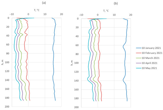
Figure 1.
Temperature distributions over the depth of two TC boreholes at different time points; TC-1 (a) and TC-2 (b).
Free convection in a vertical channel filled with fluid arises at certain critical parameters of the fluid, which are usually expressed in terms of the critical Rayleigh [11,12,13] or Grashof [14,15] numbers. Kazakov et al. [12] found that for laminar flows, the critical Rayleigh number is relatively small, with a value of about 100. Another important parameter that determines the presence of free convection is the ratio of the thermal conductivities of the fluid and the borehole casing [13].
According to [16,17], the phenomenon of free convection in boreholes can significantly distort the temperature field established in the soil surrounding the borehole. Based on a large sample of experimental data, Demezhko et al. [16] showed that convective temperature noise has a normal distribution. For this reason, to estimate the temperature deviation relative to the mean value, it is convenient to use statistical criteria, such as the standard deviation, σT, and the maximum range, ΔTmax [9,18]. In [16], the following formula was proposed:
where G is the temperature gradient, °C/m; and R is the borehole radius, m.
Thermal convection leads not only to temperature fluctuations relative to the actual temperature of the soil (which could easily be eliminated by averaging over time), but also to a long-term quasi-stationary effect (QSE) [12], which is manifested as a consistent decrease in the temperature gradient relative to its value in the soil. Demezhko et al. [17] found that the maximum gradient decrease is observed in the upper and lower parts of the borehole, with an average value of 7.5% over the length of the borehole estimated for Rayleigh numbers up to 105. At the same time, this feature may be due to insufficient calculation time and the limited volume of soil mass surrounding the borehole. In [19], an assumption was made and verified that the QSE is similar to the effect caused by the circulation of fluid during borehole drilling or flushing.
Other studies in the scientific literature have not considered the QSE. In our opinion, this effect is important for correct temperature measurements in vertical boreholes. It is not clear what local temperature errors may arise due to QSE, since only the average error has been estimated previously. It is also not known which sections of the well are most affected by the QSE. These questions are explored in this study.
Taking into account the fact that previous studies were carried out using a limited range of Rayleigh numbers, in this paper we attempted to extend our analysis to Rayleigh numbers that occur during AGF up to values in the order of 107. For this, an unsteady convective motion of a calcium chloride solution in a TC borehole is considered with a constant temperature gradient at the walls. This study focuses on an analysis of the reasons for the decrease in the temperature gradient at the mouth and bottom of vertical boreholes, which has been poorly studied.
2. Methodology
A straight vertical section of the TC borehole with a radius of 0.073 m and a length of 25 m is considered (see Figure 2). The borehole is filled with a solution of calcium chloride (CaCl2), which does not freeze at negative temperatures [20]. On the upper base of the cylindrical domain, which is a section of the borehole, a pressure outlet-type boundary condition is set. The side wall and the lower base of the cylindrical domain are smooth impermeable walls, where the zero-velocity vector is set.
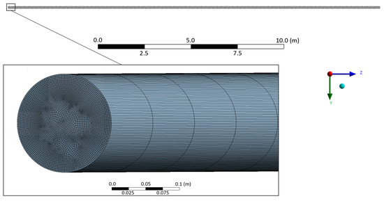
Figure 2.
Geometry of the computational domain and the mesh.
An irregular 2D mesh of quadrangular elements is built on the upper base of the cylinder. This mesh is then swept over the entire height of the borehole. A fixed number of vertical mesh layers is set, which varies from 60 to 250 depending on the density of the selected mesh. The pre-modeling on several meshes and how we selected the best option are discussed below.
The solution flow is assumed to be unsteady, incompressible, non-isothermal, and laminar. To account for thermal convection in the borehole, a gravity field and a linear dependence of the density of the solution on its temperature are set. Two concentrations of CaCl2 solution are considered: 15% and 25%.
The dependences of solution densities on temperature T for these two concentrations are as follows:
These dependences were obtained from [21] by searching for a linear approximation of the tabular values of the solution densities at different temperatures.
The other thermophysical properties of the solutions are assumed to be independent of temperature. These properties, considered at a temperature of 0 °C, are summarized in Table 1.

Table 1.
Properties of calcium chloride solutions at 0 °C.
As follows from Formulas (2) and (3), the density increases with an increase in the concentration of CaCl2 in the solution, and the dependence on temperature becomes stronger. The specific heat capacity and dynamic viscosity of the solution strongly depend on the CaCl2 concentration. The thermal conductivity of the solution changes insignificantly with increasing salt concentration in the solution. We do not take into account the temperature dependences of the specific heat capacity, thermal conductivity and dynamic viscosity of CaCl2 solutions because they are rather weak and do not affect the solution in the considered temperature range. At the same time, the dependence of density on temperature is one of the key physical factors in the problem.
The total temperature variation in the TC boreholes rarely exceeds 10 °C (see Figure 1), and therefore, the variation in solution density can be considered to be small. The Reynolds values calculated at typical fluid flow rates in a borehole (1 mm/s) are 32 for 15% CaCl2, and 21 for a 25% CaCl2 solution. Thus, for the selected parameters of the solution, the flow regime will be laminar. This allows us to formulate the problem of heat and mass transfer in a borehole in the form of the classical Boussinesq problem [22,23]. In this case, it is necessary to solve the following system of mass, momentum, and energy balance equations:
where t is the time, s; V is the water velocity vector, m/s; p is the pressure, Pa; E is the specific energy of water, J/kg; g is gravity vector, m/s2; and is the shear stress tensor, Pa, calculated by the formula:
where is the molecular viscosity of the solution, Pa·s.
This system of equations is supplemented with the following initial (IC) and boundary conditions (BC):
where G is the vertical temperature gradient at the borehole wall, °C/m; h is the height of the investigated section of the borehole, m; z is the vertical coordinate, m; R is the borehole radius, m; and r is the radial coordinate, m. The origin of the cylindrical coordinate system is at the bottom point of the borehole in the middle of its cross section.
The vertical temperature gradient G is determined based on experimental temperature measurement data along the depth of TC boreholes for the skip shaft of a potash mine under construction in the Republic of Belarus (see Figure 1). The temperature gradients of the experimentally measured temperatures along the depth of two TC boreholes are shown in Figure 3. They were calculated for temperature measurements at fixed spatial steps of 0.5 m.
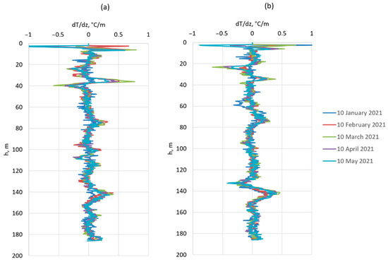
Figure 3.
Distributions of temperature gradients along the depth of TC-1 (a) and TC-2 (b) boreholes.
Analysis of the curves in Figure 3 showed that the average temperature gradient for different boreholes across time varies between 0.056 °C/m and 0.083 °C/m. The average temperature gradient was calculated by the formula:
where N is the number of measurement points.
The modular maximum temperature gradient, given by the formula:
can reach 1.3 °C/m locally. It is important to note that in determining these estimates, we did not take into account the first 2 m near the mouth of the borehole, where the gradient is very high due to the influence of atmospheric conditions. The temperature distribution dynamics in this small area are very different from those in the rest of the borehole. Notably, soil layers at a depth of more than 5 m are of the greatest interest for freezing analysis.
Based on the estimated value of G under real conditions, we further studied thermal convection in boreholes for G values ranging from 0.025 to 0.2 °C/m. Taking into account the data from Table 1, the corresponding Rayleigh numbers range from 6.8 × 10⁵ to 5 × 10⁷. The Rayleigh numbers are calculated using a formula from [12]:
where a is the thermal diffusivity, m2/s; is the coefficient of thermal expansion, °C−1; and is the kinematic viscosity, m2/s.
The numerical solutions to Equations (4)–(11) were obtained using the SIMPLE method of the Ansys Fluent 2021 program [24]. Spatial discretization was carried out using second-order schemes, while time discretization was conducted using an implicit first-order scheme.
3. Results and Discussion
First of all, we analyzed the independence of the solution from the spatial mesh and the time step. The criterion for analysis was the temperature distribution along the borehole axis for a temperature gradient of 0.2 °C/m at the wall. The temperature of the wall is 0 °C at the bottom of the borehole, and −5 °C at the mouth. The simulation time was 1 h. Figure 4 shows temperature distributions along the borehole axis for three spatial meshes and at four time steps. The data in Figure 4a was obtained using a time step of 20 s. The data in Figure 4b was obtained using a mesh of 137,280 cells. In general, it can be seen from the preliminary simulation that it was not possible to achieve identical results for any pair of calculations. However, it is important to understand that temperature fluctuations during thermal convection are quite chaotic and sensitive to many parameters of the problem. Therefore, it was important that the numerical model could correctly calculate the average amplitude of temporal temperature fluctuations in the thermal convection area and the temperature deviations near the bottom of the borehole. For this reason, a mesh of 137,280 cells was chosen. Simulations at various time steps from 5 to 40 s did not reveal a significant effect of the time step on the solution. Nevertheless, the curve in Figure 4b for the 40 s time step reflects the temperature profile near the bottom of the borehole less accurately than the other curves. Therefore, a time step of 20 s was considered for further calculations.
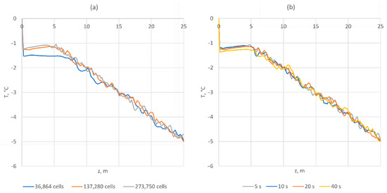
Figure 4.
Temperature distributions along the borehole axis for different spatial meshes (a) and at different time steps (b).
Next, we analyzed the temporal dynamics of the temperature distribution along the borehole axis for the selected mesh. We selected the borehole axis since this line is the farthest from the borehole walls and will most likely show the largest temperature deviations from the linear distribution specified at the wall. In addition, fiber optic cables or point sensors are usually located closer to the middle of the borehole.
Figure 5a,b shows the temperature distributions for a 15% and 25% CaCl2 solution, respectively. The temperature gradient at the wall is still 0.2 °C/m. It can be seen from Figure 5 that the initially homogeneous velocity field rapidly changes in line with the given borehole wall temperature field (black dashed line). The temperature field of the solution tends toward linearity, but it is not exactly linear due to the presence of undamped temperature fluctuations caused by thermal convection. However, as shown in [17], averaging the temporal temperature fluctuation data due to thermal convection in the center of the borehole solves this problem and allows the required linear temperature profile to be obtained.
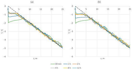
Figure 5.
Temperature distributions along the borehole axis at different times at different concentrations of CaCl2 in the solution: 15% (a) and 25% (b).
Of greatest interest is a small section of the borehole near its bottom, where the temperature of the solution near the borehole axis differs significantly from the temperature of the wall during the entire simulation time, and this is not eliminated by simple time averaging. The greatest differences are observed at the shortest time of 30 min; in this case, the length of the borehole section with a different solution temperature reaches 7 m. This effect at short times is due to the influence of the initial temperature condition. Later, the temperature field at this section of the borehole stabilizes and ceases to change with time, and the dependence on the initial conditions disappears. In this case, a section about 3–4 m in length still remains, in which the solution temperature profile differs greatly from the linear profile set at the wall. In this section, the temperature curve is almost parallel to the X axis, which indicates a value of zero for the temperature gradient G. Thus, the temperature gradient deviation along the axis of the borehole near its bottom differs from the specified temperature gradient at the walls by approximately 100%.
At the other end of the borehole, where the outlet condition is set, the fluid temperature profile corresponds closely to the wall temperature. For a time of 12 h, the measured temperature gradient along the borehole axis differs from the gradient specified at the wall by about 3–4%.
In order to understand the anomalous behavior of the fluid temperature profile near the bottom of the borehole, it is necessary to analyze the velocity and temperature fields in the transverse and longitudinal sections of the borehole. The velocity fields are shown in Figure 6 for a simulation time of 4 h and 15% CaCl2 concentration. Figure 7 shows the temperature fields for the same simulation time and CaCl2 concentration. The fluid streamlines at the bottom of the borehole are presented in Figure 8. The upstream fluid flow is marked in red, and downstream flow is marked in blue. The maximum fluid velocities are about 0.015 m/s, which corresponds to Re ≈ 480.
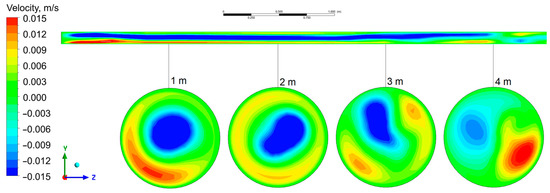
Figure 6.
Distributions of the vertical velocity component in the longitudinal and transverse cross sections of the borehole near its bottom.
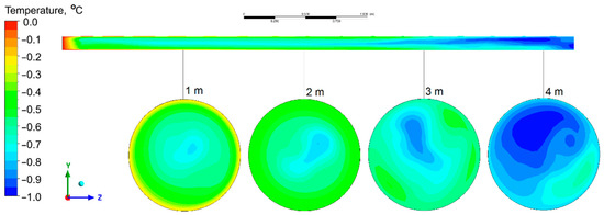
Figure 7.
Distributions of the temperature in the longitudinal and transverse cross sections of the borehole near its bottom.
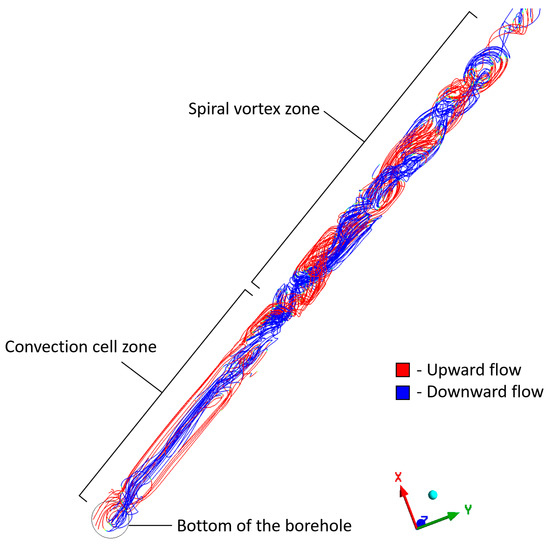
Figure 8.
Streamlines near the bottom of the borehole; the color shows the vertical direction of the flow.
It can be seen from Figure 6 and Figure 8 that in the area near the bottom of the borehole, a stable extended three-dimensional convection cell is formed with a downward flow in the center of the borehole and an upward flow near the walls. This leads to the distortion of the temperature field in the area near the axis of the borehole. The temperature is lower in the center of the cross section and higher near the borehole walls (see Figure 7). At a distance from the borehole bottom, the flow structure changes and spiral vortices are formed, the existence of which is also noted in the experimental work [16].
In the zone of a spiral vortex flow, the distribution of the vertical component of the fluid velocity in various horizontal sections is always similar and differs in rotation by some angle. This spiral structure is inevitably broken near the bottom of the borehole, because the condition of zero velocity is set on it. At the same time, due to the action of buoyancy forces in the bottom of the borehole, another convective flow structure is formed, a convection cell, which coexists well both with the zero-velocity boundary condition at the lower base of the domain and with the spiral vortex structure above.
Such an extended vortex is not formed at the borehole mouth due to the features of the boundary condition set at this boundary surface (pressure outlet). The fluid can freely flow out of and back into the computational domain through this boundary. However, if we set the condition of an impermeable wall at the mouth of the borehole, then the observed results are similar to those obtained at the bottom. As an example, Figure 9 shows the calculated temperature distributions along the borehole axis under the same boundary conditions at both ends of the borehole (in terms of the zero-velocity vector), considering a 25% CaCl2 solution.
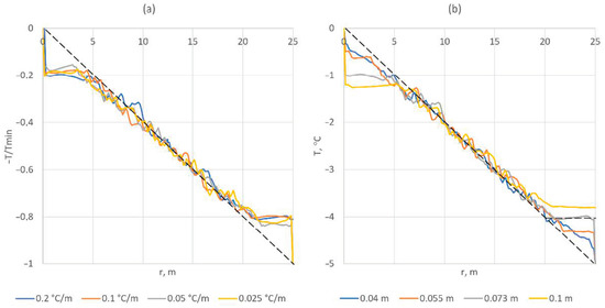
Figure 9.
Temperature distributions along the borehole axis for impermeable walls at both ends of the borehole with different temperature gradients G (a) and different borehole diameters (b).
For convenience, dimensionless temperature is marked along the Y axis in Figure 9a. This makes it possible to visually compare the temperature profiles at different temperature gradients G. Based on the data presented in Figure 9a, it can be concluded that the maximum deviation of the fluid temperature along the borehole axis from the value at its wall depends on the temperature gradient approximately according to the linear law: ΔTmax = Twall − Taxis ≈ 5 G (°C). However, the length of the temperature deviation section does not depend on G, but rather depends on the borehole radius R, as seen in Figure 9b and Table 2.
Table 2.
Lengths of the temperature deviation sections at different borehole radii.
The length of the temperature deviation section for each radius was calculated using the following method:
- An approximation of the horizontal section of the temperature curve near the borehole bottom was determined in the form T = const.
- The point of intersection of the T = const curve with the curve of Equation (11), which is a given function of wall temperature, was found. The abscissa of this intersection point was taken to be equal to the length of the temperature deviation section.
The obtained dependence of the length of the temperature deviation section on the radius R is essentially non-linear. In our opinion, it can be approximated by a logarithmic dependence of the form A + B log(R − C). For the properties of the borehole and fluid considered in this case, the parameters of this dependence are: A = 11.92, B = 2.06, and C = 0.04. These values were obtained using the least squares method [25].
From a practical point of view, a deeper study of the approximating functions for this dependence is most likely unnecessary. In this case, it is important to understand the general size of the identified area of deviation of fluid temperatures in the central region of the borehole. In the practice of AGF, boreholes with a radius of no more than 0.1 m are usually applied. This indicates that large temperature errors due to thermal convection can occur only in the lower section of a borehole up to 6 m in length. Experimental measurements of fluid temperature in a borehole can lead to an underestimation of the actual temperature at the walls of no more than 5 G (°C). This conclusion is valid only in the case of a negative temperature gradient along the borehole height: dT/dz < 0.
In fact, during AGF, there are alternating sections with positive and negative temperature gradients. Nevertheless, near the bottom of the TC borehole, a negative temperature gradient should be observed more often. This is related to the influence of the Earth’s heat flow on the lower part of the FW.
Another important consideration is that, in practice, temperature sensors may not be located in the center of the borehole cross section but can be shifted to its wall. Generally speaking, the position of the DTS cable in the cross section is an indeterminate parameter. Hence, we considered the most pessimistic scenario for the deviation of temperatures measured in the center of the borehole from the temperatures at the wall. In addition, the measuring cable itself (at a certain thickness) can influence the structure of convective currents in the borehole. This issue is not considered in this work and requires separate investigation.
4. Conclusions
From the simulation of thermal convection of a calcium chloride solution in a TC borehole, the following interesting and important results were obtained:
- An area near the borehole bottom was identified where the fluid temperature at the borehole axis deviates significantly from the temperature at the wall. This effect is observed when the boundary condition of an impermeable wall is set at the lower base of a cylindrical borehole. A similar effect is observed at the mouth of the borehole if the impermeable wall condition is set at the upper base of the cylindrical region.
- An analysis of the structure of the fluid flow in the borehole was carried out. Based on this analysis, we determined that the extended vortex is formed at the bottom of the borehole with a downward flow of fluid in the central part of the cross section and an upward flow of fluid near its walls. At the same time, in the rest of the borehole, the fluid flow is characterized by a system of helical jets, which is in agreement with data reported in the literature.
- The maximum deviations of the fluid temperature from the temperature of the walls near the bottom of the borehole and the length of the temperature deviation sections were determined. The proposed formula for calculating the magnitude of deviations will be useful for specialists in monitoring the Earth’s thermal field and artificial ground freezing.
Author Contributions
Conceptualization, M.S. and L.L.; methodology, M.S. and L.L.; software, M.S.; validation, M.S.; formal analysis, M.S.; investigation, M.S.; resources, M.S. and L.L.; data curation, M.S. and L.L.; writing—original draft preparation, M.S.; writing—review and editing, L.L.; visualization, M.S.; supervision, L.L.; project administration, L.L.; funding acquisition, M.S. and L.L. All authors have read and agreed to the published version of the manuscript.
Funding
This research was funded by Russian Science Foundation, grant number 19-77-30008.
Data Availability Statement
Not applicable.
Conflicts of Interest
The authors declare no conflict of interest.
References
- Semin, M.; Golovatyi, I.; Pugin, A. Analysis of Temperature Anomalies during Thermal Monitoring of Frozen Wall Formation. Fluids 2021, 6, 297. [Google Scholar] [CrossRef]
- Holden, J.T. Improved Thermal Computations for Artificially Frozen Shaft Excavations. J. Geotech. Geoenviron. Eng. 1997, 123, 696–701. [Google Scholar] [CrossRef]
- Nicotera, M.V.; Russo, G. Monitoring a deep excavation in pyroclastic soil and soft rock. Tunn. Undergr. Space Technol. 2021, 117, 104130. [Google Scholar] [CrossRef]
- Levin, L.; Golovatyi, I.; Zaitsev, A.; Pugin, A.; Semin, M. Thermal monitoring of frozen wall thawing after artificial ground freezing: Case study of Petrikov Potash Mine. Tunn. Undergr. Space Technol. 2021, 107, 103685. [Google Scholar] [CrossRef]
- Russo, G.; Corbo, A.; Cavuoto, F.; Autuori, S. Artificial Ground Freezing to excavate a tunnel in sandy soil. Measurements and back analysis. Tunn. Undergr. Space Technol. 2015, 50, 226–238. [Google Scholar] [CrossRef]
- Zhelnin, M.S.; Plekhov, O.A.; Semin, M.A.; Levin, L.Y. Numerical Solution for an Inverse Problem about Determination of Volumetric Heat Capacity of Rock Mass during Artificial Freezing. PNRPU Mech. Bull. 2017, 4, 56–75. [Google Scholar] [CrossRef]
- Pavlov, A.V. Estimation of temperature measurement errors of grounds in shallow boreholes in permafrost. Earth Cryosphere 2006, 4, 9–13. [Google Scholar]
- Semin, M.; Levin, L.; Bogomyagkov, A.; Pugin, A. Features of Adjusting the Frozen Soil Properties Using Borehole Temperature Measurements. Model. Simul. Eng. 2021, 2021, 8806159. [Google Scholar] [CrossRef]
- Diment, W.H. Thermal Regime of a Large Diameter Borehole: Instability of the Water Column and Comparison of Air- and Water-Filled Conditions. Geophysics 1967, 32, 720–726. [Google Scholar] [CrossRef]
- Sammel, E.A. Convective Flow and its Effect on Temperature Logging in Small-Diameter Wells. Geophysics 1968, 33, 1004–1012. [Google Scholar] [CrossRef]
- Buchberg, H.; Catton, I.; Edwards, D.K. Natural Convection in Enclosed Spaces—A Review of Application to Solar Energy Collection. J. Heat Transf. 1976, 98, 182–188. [Google Scholar] [CrossRef]
- Kazakov, B.P.; Shalimov, A.V. Stability of Convective Ventilation after Fan Switching-Off in Mines. J. Min. Sci. 2019, 55, 626–633. [Google Scholar] [CrossRef]
- Eppelbaum, L.V.; Kutasov, I.M. Estimation of the effect of thermal convection and casing on the temperature regime of boreholes: A review. J. Geophys. Eng. 2011, 8, R1–R10. [Google Scholar] [CrossRef]
- Popiel, C.O. Free Convection Heat Transfer from Vertical Slender Cylinders: A Review. Heat Transf. Eng. 2008, 29, 521–536. [Google Scholar] [CrossRef]
- Gershuni, G.Z.; Zhukhovitskii, E.M.; Tarunin, E.L. Numerical investigation of convective motion in a closed cavity. Fluid Dyn. 1966, 1, 38–42. [Google Scholar] [CrossRef]
- Demezhko, D.Y.; Khatskevich, B.D.; Mindubaev, M.G. Experimental estimation of temperature noise caused by free thermal convection in water-filled boreholes. Bull. Tomsk. Polytech. Univ. Geo Assets Eng. 2020, 331, 136–143. [Google Scholar]
- Demezhko, D.Y.; Mindubaev, M.G.; Khatskevich, B.D. Thermal effects of natural convection in boreholes. Russ. Geol. Geophys. 2017, 58, 1270–1276. [Google Scholar] [CrossRef]
- Cermak, V.; Bodri, L.; Safanda, J. Precise temperature monitoring in boreholes: Evidence for oscillatory convection? Part II: Theory and interpretation. Int. J. Earth Sci. 2008, 97, 375–384. [Google Scholar] [CrossRef]
- Demezhko, D.Y.; Khatskevich, B.D.; Mindubaev, M.G. Quasi-stationary effect of free thermal convection in water-filled boreholes. Bull. Tomsk. Polytech. Univ. Geo Assets Eng. 2021, 332, 131–139. [Google Scholar]
- Martin, J.; Clayton, C.J.; Murphy, B.A. Method for Deriving Sub-Permafrost Groundwater Salinity and Total Dissolved Solids. In Proceedings of the Mine Water Solutions Conference, Lima, Peru, 15–17 April 2013. [Google Scholar]
- Chubik, I.A.; Maslov, A.M. Handbook on the Thermophysical Characteristics of Foodstuffs and Semi-Finished Products; Pyshevaya promyshlennost: Moscow, Russia, 1970. (In Russian) [Google Scholar]
- Mayeli, P.; Sheard, G.J. Buoyancy-driven flows beyond the Boussinesq approximation: A brief review. Int. Commun. Heat Mass Transf. 2021, 125, 105316. [Google Scholar] [CrossRef]
- Gustafsson, A.M.; Westerlund, L.; Hellström, G. CFD-modelling of natural convection in a groundwater-filled borehole heat exchanger. Appl. Therm. Eng. 2010, 30, 683–691. [Google Scholar] [CrossRef] [Green Version]
- Fletcher, C.A. Computational Techniques for Fluid Dynamics 2: Specific Techniques for Different Flow Categories; Springer Science & Business Media: Berlin, Germany, 2012. [Google Scholar]
- Björck, Å. Numerical Methods for Least Squares Problems; Society for Industrial and Applied Mathematics: Philadelphia, PA, USA, 1996. [Google Scholar]
Publisher’s Note: MDPI stays neutral with regard to jurisdictional claims in published maps and institutional affiliations. |
© 2022 by the authors. Licensee MDPI, Basel, Switzerland. This article is an open access article distributed under the terms and conditions of the Creative Commons Attribution (CC BY) license (https://creativecommons.org/licenses/by/4.0/).