Probability Distribution of Extreme Events in a Baroclinic Wave Laboratory Experiment

Abstract

Atmospheric westerly jet streams are driven by temperature differences between low and high latitudes and the rotation of the Earth. Meandering jet streams and propagating Rossby waves are responsible for the variable weather in the mid-latitudes. Moreover, extreme weather events such as heat waves and cold spells are part of the jet stream dynamics. For many years, a simple analog in the form of a simplified laboratory experiment, the differentially heated rotating annulus, has provided insight into the dynamics of the meandering jet stream. In the present study, probability density distributions of extreme events from a long-term laboratory experiment are studied and compared to the atmospheric probability density distributions. Empirical distributions of extreme value monthly block data are derived for the experimental and atmospheric cases. Generalized extreme value distributions are adjusted to the empirical distributions, and the distribution parameters are compared. Good agreement was found, but the distributions of the experimental data showed a shift toward larger extreme values, and some explanations for this shift are suggested. The results indicate that the laboratory model might be a useful tool for investigating changes in extreme event distributions due to climate change. In the laboratory context, the change can be modeled by an increase in total temperature accompanied by a reduction in the radial heat contrast.

1. Introduction

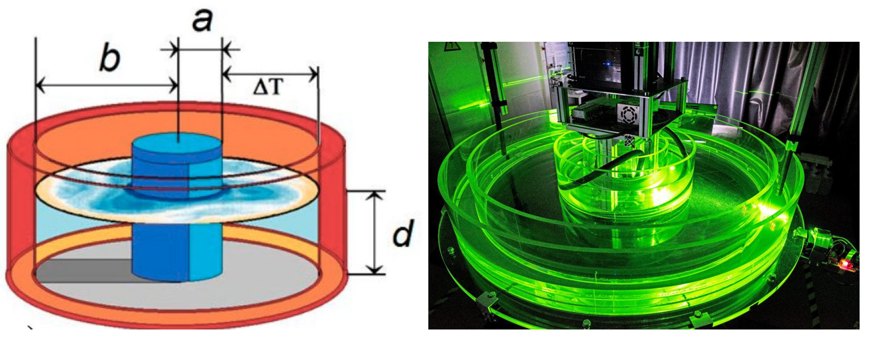
In the late 1940s, dishpan experiments were started to simulate large-scale atmospheric motions. The authors of [1] used a rotating cylindrical vessel with a flat bottom and top. In these experiments, the radial temperature difference, maintained by using ice cubes for the inner part, was hard to control. In [2], a rotating annular vessel consisting of three concentric cylinders was used (see Figure 1), where the narrow gap outer annulus was filled with warm fluid, the inner cylinder was filled with cold fluid, and the central part was the experimental chamber filled with water or silicon oil. Temperature control was rather easy, and hence this kind of experiment was conducted in later years by a large number of researchers [3,4]. In [5], the now famous stability diagram was derived, where the thermal Rossby number ($R{o}_T$) was plotted against the Taylor number ($Ta$) (see Equation (1)) in a double-logarithmic scale. The former measures the thermal wind speed against the rotation speed, and the latter plays the role of the Reynolds number for rotating flows. In fact, these two non-dimensional parameters are the similarity parameters that connect the experiment with real atmospheric flows (i.e., the former needs to be small and the latter large for similarity with atmospheric flows). The parameters read as follows:

$$R{o}_T=\frac{gd\Delta \rho }{{\rho }_0{\mathsf{\Omega }}^2{(b-a)}^2},Ta=\frac{4{\mathsf{\Omega }}^2{(b-a)}^5}{{\nu }^{2}d}.$$

(1)

where $\Delta \rho ={\rho }_0\alpha \Delta T$ and g is the constant of gravity. All the other variables are given in

Table 1. Parameters of the laboratory experiment. See also Figure 1 (left).

Geometry
	inner radius	a (mm)	350
	outer radius	b (mm)	700
	gap width	b–a (mm)	350
	fluid depth	d (mm)	60
Exp. Parameters
	temperature difference	$\Delta T$ (K)	4.0
	revolution speed	$\mathsf{\Omega }$ (rpm)	2.0
Fluid Properties
	density	$\rho$ ($\mathrm{kg}{\mathrm{m}}^{-3}$)	997
	kin. viscosity	$\nu$ (${\mathrm{m}}^2{\mathrm{s}}^{-1}$)	1.004 $\times {10}^{-6}$
	therm. conductivity	$\kappa$ (${\mathrm{m}}^2{\mathrm{s}}^{-1}$)	0.1434 $\times {10}^{-6}$
	exp. coefficient	$\alpha$ (1/K)	0.207 $\times {10}^{-3}$
Similarity Parameters
	Prandtl number	Pr = $\nu /\kappa$	7.00
	Rossby number	Ro	0.91 $\times {10}^{-2}$
	Taylor number	Ta	1.52 $\times {10}^{10}$

.

Using Hide’s annulus experiment, many aspects of atmospheric flows have been studied. The starting point was the confirmation of linear baroclinic instability as a key process of large-scale dynamics [5], but nonlinear regime transitions and bifurcations to chaotic flows have also been analyzed [8]. The nonlinear saturation of baroclinic waves [9], wave-mean flow, and wave-wave interactions [10] was also of interest. In addition, vacillations and low-frequency variability [11] have been investigated intensively. More recently, ideas for the optimal growth of baroclinic waves were tested [12]. Moreover, secondary instabilities of the baroclinic jet and the generation of internal gravity waves have been studied [13].

This series of successful research showed that the rotating annulus is a good analog to atmospheric dynamics, and this encouraged experiment-oriented geoscientists to study climate-related processes as well. The ideas in [14] on blocking were tested experimentally [15]. In meteorology, blocking describes the development of large-scale patterns in atmospheric pressure that are almost stationary and block or redirect migratory cyclones. Thermally and orographically forced baroclinic waves and the formation of blocking by wave triads have been studied [16]. The authors of [17] experimentally investigated the temperature distribution for open and closed baroclinic annulus flows as an analog to Drake passage opening scenarios relevant in paleooceanography. Aside from these dynamical aspects of atmospheric and climatic extreme events, more statistical features came into the focus as well. For instance, the authors of [6,18] studied the baroclinic jet variability in so-called polar amplification scenarios. However, to our knowledge, no quantitative data analysis on the distribution of extreme events has been conducted so far using the annulus experiment. This is the topic of the present work.

In Section 2, we briefly give the experimental set-up, and in Section 3 we present the experimental data retrieved from the annulus experiment, which form the basis of our extreme value statistics. In Section 4, we present the main results and show the extreme value distributions for the experimental data. We further compare these distributions with the one obtained from the reanalysis atmospheric data. In Section 5, we give our conclusions.

2. Experimental Set-Up

The experiment used is a classical Hide set-up with three concentric cylinders (see Figure 1). The fluid used for heating and cooling as well as the working fluid in the central annular chamber was water. The water in the inner cylinder (outer annulus) was cooled (heated). In contrast to our earlier experiments with applications to climate [6,17,18], we used a larger tank with features closer to the atmospheric dynamics [13,19]. The experimental set-up is described in detail in [20] and will not be repeated here. All the relevant experimental parameters can be found in Table 1. For the dimensionless parameters of the Earth atmosphere, it is not straightforward to apply Equation (1). However, a rough estimate for the atmosphere gives $Pr=0.78$, $Ro={10}^{-2}$, and $Ta=3\times {10}^{31}$. The large $Ta$ results from the fact that the mid-latitude belt is a few thousand kilometers wide, and this width occurs at the fifth power in the equation. Hence, when comparing these parameters, we find that the experiment and the atmosphere fulfill an incomplete similarity only. In fact, applying a sound dimensional analysis would give more than 10 dimensionless parameters [21], and it seems a bit naive to project the atmospheric dynamics to only three parameters. However, empirical experience in the laboratory justifies this approach [4]. We can say that, when following the diagram in [5], with $1<Pr<10$, $Ro\ll 1$, and $Ta\to \infty$, the experiment and the atmosphere as well are in a geostrophic turbulent regime showing similar dynamics.

3. Data

We started the experiment by heating and cooling the outer and inner walls, respectively. Reaching a stable radial temperature gradient took about 5 h. Subsequently, rotation was started. The spin-up time was $L/{\left(\mathsf{\Omega }\nu \right)}^{1/2}\approx 15$ min when using $L=0.35$ m, $\mathsf{\Omega }=2$ rpm, and $\nu ={10}^{-6}$ m${}^2$ s. The period for heating and spin-up was excluded from the analysis. The surface temperature was measured by an infrared (IR) camera (see

Table 2. Infrared camera’s technical specifications. The infrared camera used was from Jenoptik, module IR-TCM 640. The software was the IRBIS package developed by InfraTec GmbH, Dresden, Germany.

Image format	1024 × 680 pixel
Spectral range	7.5–14 $\mathsf{\mu }$m
Range for measuring and visualization	$233.15$–$573.15$ K
Thermal sensitivity	<80 mK
Measurement accuracy	±1.5 K
Dynamic range	16 bit
Image rate	60 Hz

for details). The total experimental run lasted for 24 h with a sampling rate of $\Delta t=30$ s (one IR image per rotation). Taking the angular tank velocity of 2 rpm into account, this corresponded to a time period of about 7.9 years of observation. The IR-camera recorded the surface temperature data only for a segment of the full annulus, as shown in Figure 2 (left). To give the reader an impression of the surface temperature dynamics, we display a Hovmoeller plot over a time period of 1 h from day 380 to day 500 (Figure 2 (right)). The data were taken along the azimuthal line segment shown in magenta in Figure 2 (left). Counterclockwise-traveling baroclinic waves could be identified. However, the wave pattern was rather irregular, which is typical for the regime of geostrophic turbulence.

For the extreme value statistics, the data were processed in the following way. First, we computed the spatial mean $E_i$ and the spatial variance $V_i$ for each day (i.e., once per revolution) $i=1,2,\dots ,2880$ of the series of IR-images. Each image contained temperature values in matrix form. In total, we had 2880 matrices of a size $680\times 1024$. Second, we evaluated the maximum values in a data segment called a “block” (here, we chose 1 month as the block length):

$$E_{ext}\left(j\right)=max(\left\{E_i\right\}\mid i\mathrm{within}\mathrm{jth}\mathrm{month}\mathrm{of}\mathrm{the}\mathrm{time}\mathrm{series}),$$

(2)

$$V_{ext}\left(j\right)=max(\left\{V_i\right\}\mid i\mathrm{within}\mathrm{jth}\mathrm{month}\mathrm{of}\mathrm{the}\mathrm{time}\mathrm{series}).$$

(3)

This yielded 96 $E_{ext}$ and 96 $V_{ext}$ as values of the extreme spatial mean temperature and spatial temperature variance, respectively. Note that a “month” corresponds to 30 revolutions of the tank. Finally, we considered the deviation from the mean values:

$$\begin{array}{ccc}\hfill E_{ext}^{\prime }\left(j\right)& =& E_{ext}\left(j\right)-{\langle E\rangle }_j,j=1,2,\dots ,96,\hfill \end{array}$$

(4)

$$\begin{array}{ccc}\hfill V_{ext}^{\prime }\left(j\right)& =& V_{ext}\left(j\right)-{\langle V\rangle }_j,j=1,2,\dots ,96,\hfill \end{array}$$

(5)

where ${\langle E\rangle }_j$ and ${\langle V\rangle }_j$ denote the monthly mean values of the spatial mean and variance, respectively.

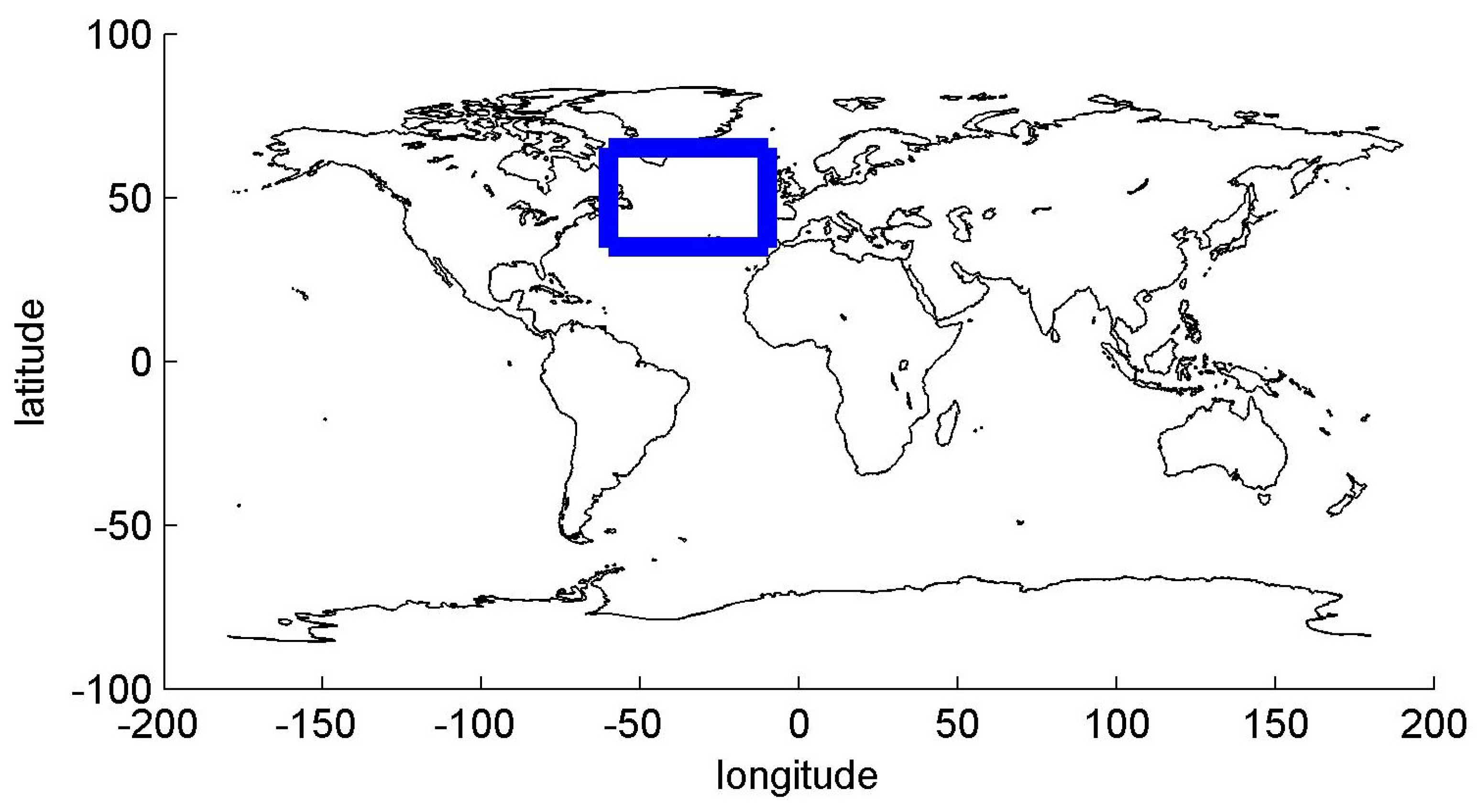
For a later comparison with extreme value distributions in real atmospheric flows, we used NCEP reanalysis data (PSL Climate Data Repository/Public/PSL Datasets/PSL Gridded Datasets/ncep.reanalysis) from the 8-year period of 2013–2020. We considered the daily mean temperature data from the tropopause level of the North-Atlantic sector (see Figure 3). This sector is not affected much by the topography, which was absent in the experiment. Note that moving the sector to a continental region with highly mountainous terrain would affect the results, since the topography can have a significant impact on the jet flow. On the other hand, a corresponding sector over the Pacific region gave similar results. Note further that data from the upper troposphere have been shown to be closer to the experimental data since their surface effects are less prominent. Recently, it has been shown in [13] that wave energy contributions from the upper atmosphere are qualitatively comparable to upper level experimental data. Using the NCEP data, we generated the same block data of E and V as given by Equations (4) and ().

4. Results

4.1. Extreme Value Distributions

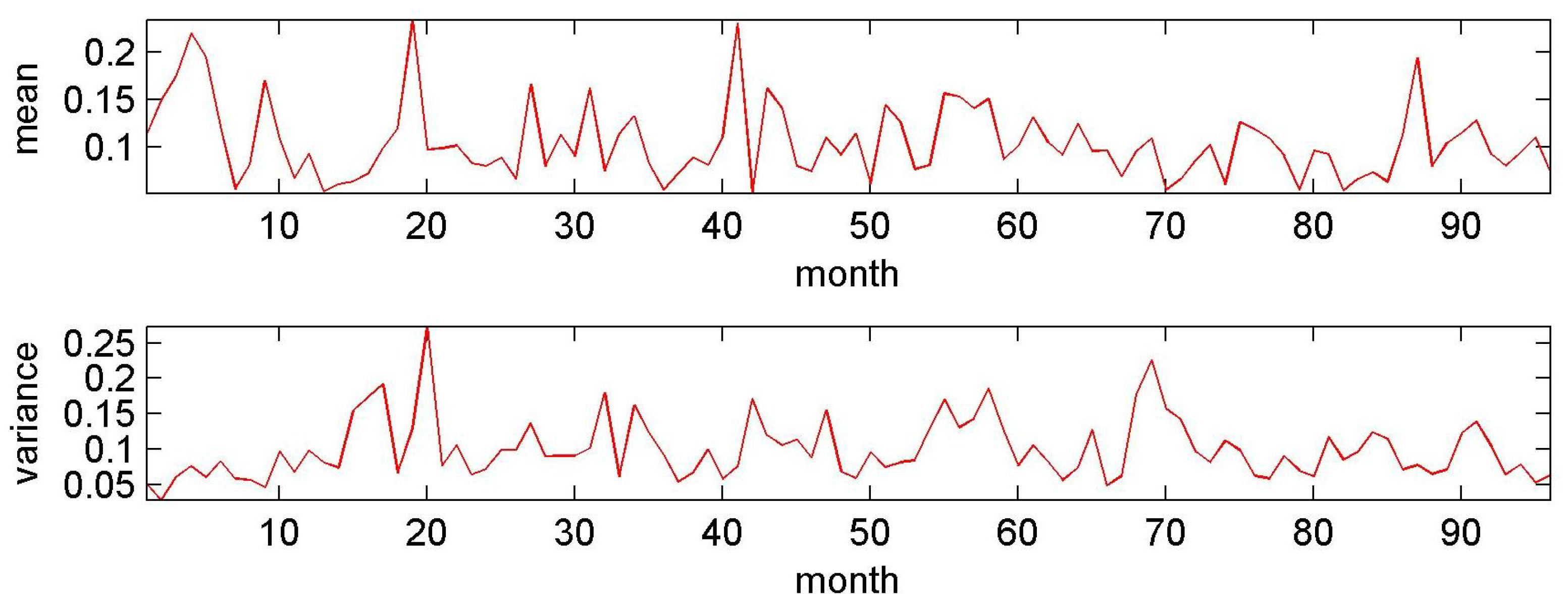
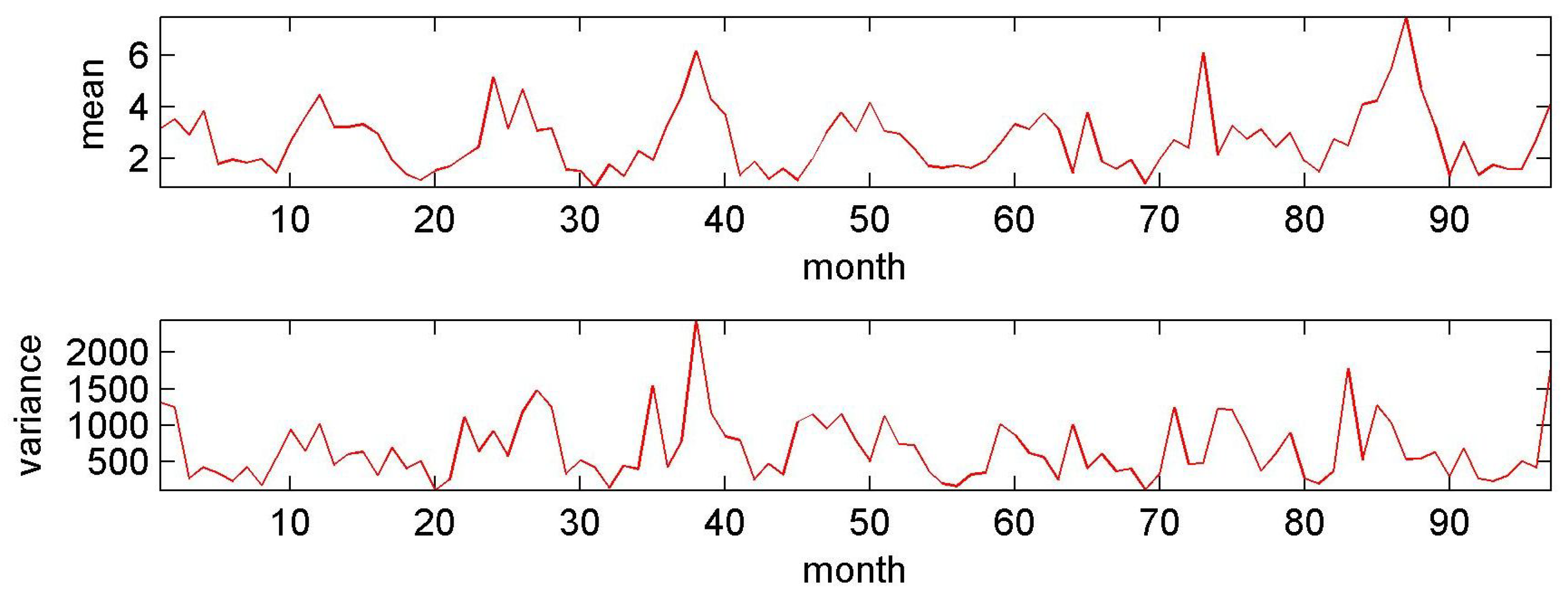
The block data of the extremes of the mean temperature and variance $E_{ext}^{\prime }\left(j\right)$ and $V_{ext}^{\prime }\left(j\right)$ are shown for the experiment in Figure 4 and for the NCEP data in Figure 5. Note that the variance of the atmospheric NCEP data was much larger than the experimental variance. Spatial temperature differences along the tropopause above the Atlantic region (see Figure 3) can be large, and they were much larger than the temperature gradients in the experimental surface layer. Therefore, the spatial variance can be above 2000 K${}^2$ for the NCEP region, but it was only about $0.2$ K${}^2$ for the section of the annulus considered.

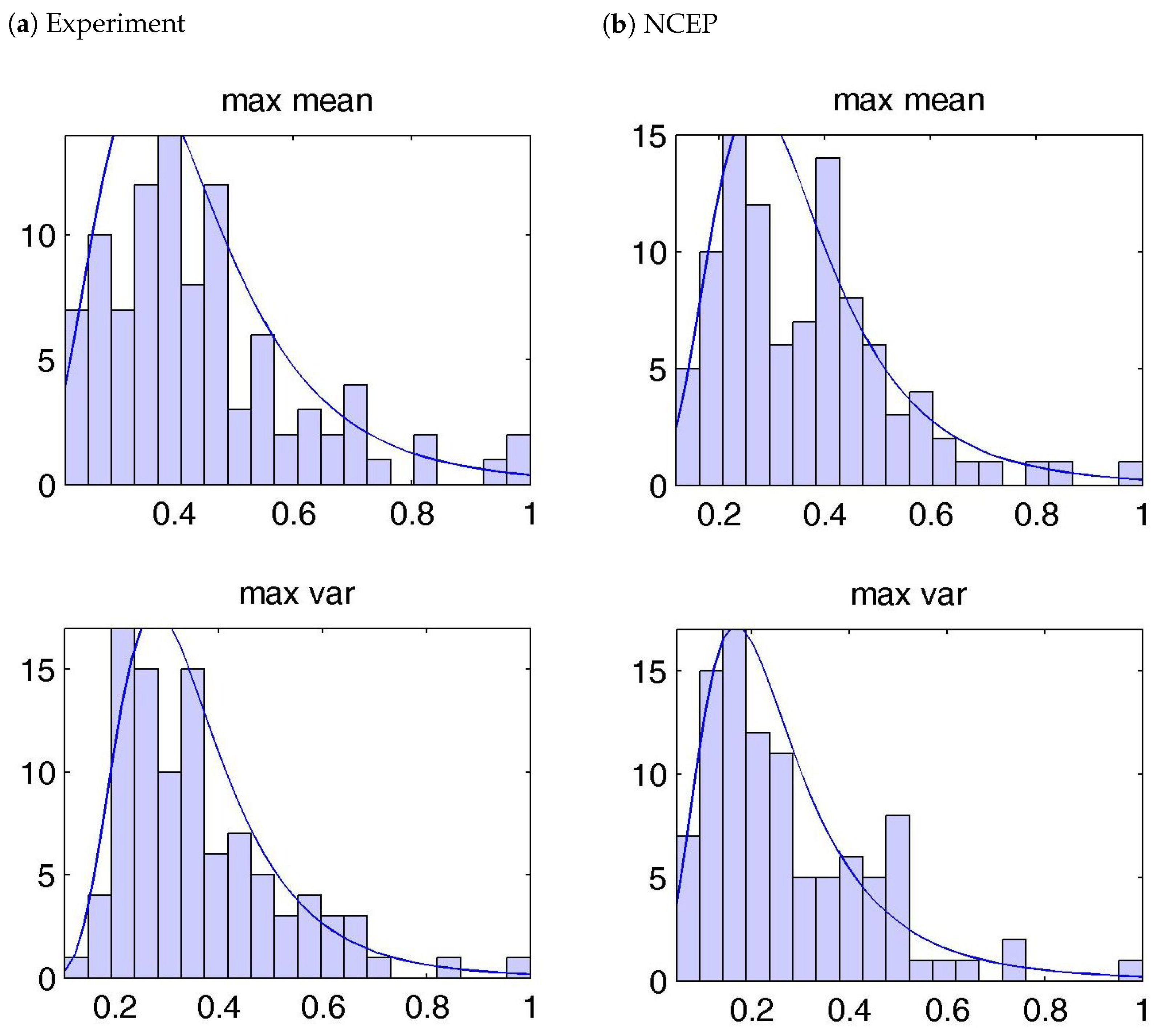
Next, we divided the range of $E_{ext}^{\prime }\left(j\right)$ and $V_{ext}^{\prime }\left(j\right)$ values into 20 classes and evaluated the empirical probability distributions with these block data. For a better comparison, we scaled $E_{ext}^{\prime }\left(j\right)$ by

$$\mid \left(max(\left\{E_{ext}^{\prime }\left(j\right)\right\}\mid j=1,2,\dots 96)\right)\mid ,$$

(6)

which was the absolute value of the maximum of all 96 $E_{ext}^{\prime }\left(j\right)$ values. For $V_{ext}^{\prime }\left(j\right)$ and the NCEP distributions, we applied the corresponding scaling. The distributions for the experimental data (NCEP data) are shown in Figure 6’s left column (right column). By inspection, we found a good qualitative similarity between the experimental and the atmospheric data.

For a more quantitative comparison, we fitted the generalized extreme value (GEV) distribution to the empirical distributions shown in Figure 6. This allowed us to contrast the parameters and hence quantitatively check the agreement between the experimental and atmospheric distributions. The GEV distribution is the standard choice for block data extremes, whereas the generalized Pareto (GP) distribution is more common for peaks-over-threshold (POT) data, which were not considered here.

The GEV distribution reads as follows:

$$F_{GEV}\left(x\right)=\left\{\begin{array}{cc}exp\left(-{\left(1+\xi (x-\mu )/\sigma \right)}^{-1/\xi }\right)\hfill & for\xi \ne 0,\hfill \\ exp\left(-exp\left(-(x-\mu )/\sigma \right)\right)\hfill & for\xi =0,\hfill \end{array}\right.$$

(7)

where $\xi$ is the shape parameter, $\sigma$ is the scale parameter, and $\mu$ is the location parameter.

In

Table 3. Estimated parameters for the GEV distribution and the confidence intervals at a 95% confidence level.

	$\mathit{\xi }$	$\mathit{\sigma }$	$\mathit{\mu }$	${\mathit{\xi }}_{95\%}^{\pm }$	${\mathit{\sigma }}_{95\%}^{\pm }$	${\mathit{\mu }}_{95\%}^{\pm }$
GEV${}_{exp}^E$	0.1230	0.1157	0.3621	−0.0585	0.0967	0.3353
				0.3044	0.1384	0.3889
GEV${}_{exp}^V$	0.1136	0.1055	0.2903	−0.0387	0.0890	0.2666
				0.2660	0.1252	0.3140
GEV${}_{ncep}^E$	0.1204	0.1161	0.2809	−0.0800	0.0965	0.2536
				0.3207	0.1396	0.3082
GEV${}_{ncep}^V$	0.1996	0.1115	0.1870	−0.0020	0.0922	0.1608
				0.4012	0.1347	0.2131

, we display $\xi$, $\sigma$, and $\mu$ for the experimental (upper two rows, GEV${}_{exp}^{E,V}$) and the atmospheric (lower two rows, GEV${}_{ncep}^{E,V}$) extreme value distributions. They were estimated by using the MATLAB function gevfit with maximum likelihood estimation (for details, see, for example, [22,23]). We further show the confidence intervals of these parameters (${\xi }_{95\%}^{\pm }$, ${\sigma }_{95\%}^{\pm }$, ${\mu }_{95\%}^{\pm }$) at a 95% confidence level.

4.2. Discussion

From Table 3, we see good agreement between the experimental and atmospheric parameters. This holds in particular for the first moment (extremes of spatial means) (i.e., when comparing GEV${}_{exp}^E$ and GEV${}_{ncep}^E$). The largest deviation could be found for $\mu$ (i.e., the locations of the distribution centers differed somewhat from each other). For all parameters, there was uncertainty, which was largest for $\xi$. Such uncertainties come from the fact that the series of monthly extreme values from an 8-year long series are rather short, and longer experimental runs should be performed in the future.

For the second moment (extremes of spatial variances), the agreement was a bit weaker but still surprisingly good. Here, ten largest deviations could be found for $\xi$ and $\mu$. Additionally, the uncertainties were comparable to the ones of the first moment and were again largest for $\xi$.

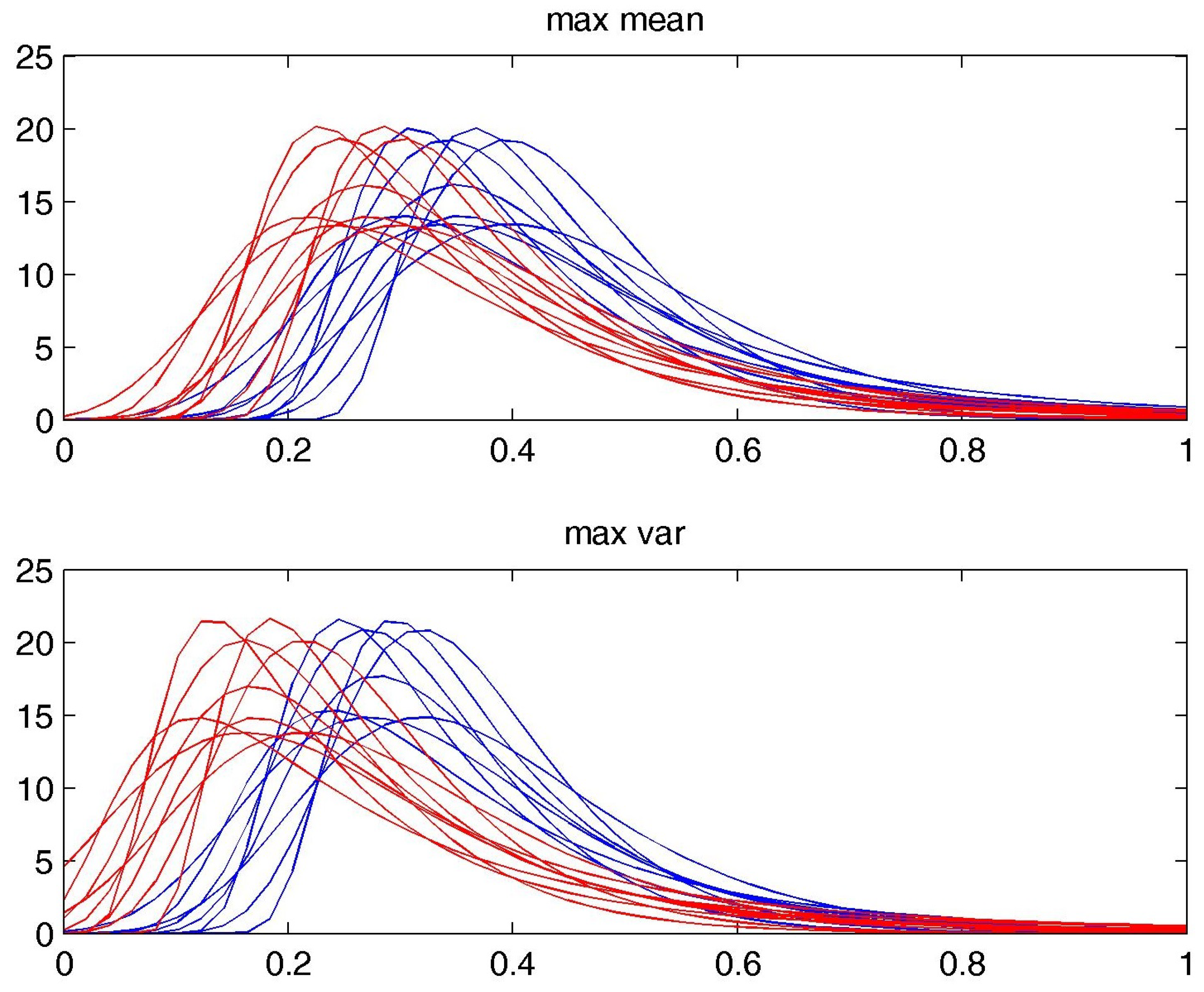
To make the comparison between the extreme value distributions of the experimental and atmospheric NCEP data more transparent, we plotted in Figure 7 the distributions for all possible parameter combinations of the parameters given in Table 3 (i.e., [${\xi }_{95\%}^{+}$${\sigma }_{95\%}^{+}$${\mu }_{95\%}^{+}$], [${\xi }_{95\%}^{-}$${\sigma }_{95\%}^{+}$${\mu }_{95\%}^{+}$], [${\xi }_{95\%}^{-}$${\sigma }_{95\%}^{-}$${\mu }_{95\%}^{+}$],...), giving eight curves for each GEV. In blue, the experimental distributions are displayed. In red, the atmospheric distributions are shown. In the upper figure, we see the distributions of $E^{\prime }$, and in the lower one, the distributions of $V^{\prime }$ are shown. Obviously, as mentioned above, there was a systematic shift between the distributions. With respect to the atmospheric distributions, the experimental distributions shifted toward larger $E^{\prime }$ and $V^{\prime }$ values, respectively. However, note that there is also an overlap between the distributions.

Why was the probability for values between 0.2 and 0.4 larger for the experimental data than for the atmospheric data? Of course, it cannot be expected that the distributions are equal, since there are many processes in the atmosphere influencing extreme conditions not included in the simple laboratory experiment. The significant differences are the missing beta effect and the large Prandtl number in the experiment. Due to the beta effect, the flow was more dispersive, which might have weakened the chance for extremes. The large $Pr$ led to more complex flow patterns [24] that might have enhanced the number of extremes. One other significant difference between the experiment and the atmospheric case is the missing land–sea contrast in the experiment. This contrast leads to the development of stationary waves in the atmosphere that can interact with the propagating Rossby wave and meander to form meteorological blocking events. The blocking phenomenon (i.e., the formation of nearly stationary pressure patterns) affects the frequency of heat waves and cold spells. This effect was not included in the experimental flow. Nevertheless, the rather good match of the extreme distribution is a promising fact for laboratory studies on the impact of climate change on the frequency of extreme events. In the lab, climate change can easily be simulated by increasing the temperature and, at the same time, reducing $\Delta T$ to mimick the effect of arctic amplification, which reduces the north-south temperature gradient of the Northern Hemisphere [6,18].

Finally, we note that for higher moments, such as skewness and kurtosis, the distributions of the experiment and atmosphere differ more. It is likely that for the higher moments, the time series are too short to obtain robust extreme value distributions.

5. Conclusions

It is well known that the dynamics of atmospheric baroclinic waves was well represented in the rotating annulus experiment, and the jet found in the experiment shares many features with its atmospheric counterpart. This might be surprising since a cylindrical tank bears, at first sight, little resemblance with a spherical planetary system [21]. However, the $\beta$ effect resulting from the spherical shape of the Earth modifies the process of baroclinic instability but is not essential for the formation of long waves in the atmosphere. The famous Eady model that can be considered as the theoretical basis for baroclinic wave and jet formation neglects the $\beta$ effect as well [25].

Laboratory experiments do not apply physical simplifications or parameterizations of physical processes but have other shortcomings compared with numerical simulations, which we do not want to discuss in detail here. In any case, using the experiment makes it possible to produce an independent dataset to study the response of the jet flow to changing boundary conditions. Such data are not intended to replace numerical data, but they can complement them. We thus have an independent data source whose analysis can improve our insight into climate-relevant processes, such as the occurrence of extreme events.

In the present paper, we studied the daily surface temperature data (one dataset per revolution) from a 24-h thermally driven rotating annulus experiment to derive probability density distributions of extreme values. We considered the maximum spatial means and variances within 96 blocks of a length of 1 month (30 revolutions of the tank). Following extreme value theory, the data could be fit to the generalized extreme value (GEV) distribution. This distribution has three parameters: the shape parameter $\xi$, the scale parameter $\sigma$, and the location parameter $\mu$. We compared the parameters to the ones from an 8-year series of daily atmospheric data, which we subjected to the exact same statistical procedure. We found the parameters to be comparable, demonstrating that the differentially heated rotating annulus is a promising tool for investigating extreme events in the atmosphere.

As for the meandering flow in the experiment, atmospheric jet streams are driven by north-south temperature differences and rotation. Climate change is weakening the north-south temperature gradient, a feature coined Arctic amplification. It might well be that a weakened jet stream shows more meanders, which may increase the probability for extreme events such as atmospheric blocking. However, considering the upper levels of the troposphere and lower levels of the stratosphere, the north-south temperature gradient might even increase, which then might imply less frequent extreme events [26]. These are open questions that are usually tackled by numerical modeling. However, in light of our results and the fact that the radial temperature gradient can experimentally be controlled, the rotating annulus laboratory experiment might also be a useful additional tool studying the impact of large-scale climate change on the occurrence of extreme events.

References

1. Fultz, D.; Long, R.R.; Owens, G.V.; Weil, J. Two-dimensional flow around a circular barrier in a rotating shell. AMS Meteorol. Monogr. 1959, 4, 61–68. [Google Scholar]
2. Hide, R. Some experiments on thermal convection in a rotating liquid. Q. J. R. Meteoro. Soc. 1953, 79, 294–297. [Google Scholar] [CrossRef]
3. Harlander, U.; von Larcher, T.; Wright, G.B.; Hoff, M.; Alexandrov, K.; Egbers, C. Chapter 17—Orthogonal decomposition methods to analyze PIV, LDA, and Thermography data of thermally driven rotating annulus laboratory experiments. In Modeling Atmospheric and Oceanic Flows: Insight from Laboratory Experiments and Numerical Simulations; von Larcher, T., Williams, P.D., Eds.; Wiley: Hoboken, NJ, USA, 2014; pp. 315–337. [Google Scholar]
4. Read, P.L.; Perez, E.P.; Moraz, I.M.; Young, R.M.B. Chapter 1—Circulation of planetary atmospheres: Insights from rotating annulus and related experiments. In Modeling Atmospheric and Oceanic Flows: Insight from Laboratory Experiments and Numerical Simulations; von Larcher, T., Williams, P.D., Eds.; Wiley: Hoboken, NJ, USA, 2014; pp. 9–45. [Google Scholar]
5. Folis, W.W.; Hide, R. Thermal convection in a rotating annulus of liquid: Effect of viscosity on the transition between axisymmetric and non-axisymmetric flow regimes. J. Atmos. Sci. 1965, 22, 541–558. [Google Scholar]
6. Vincze, M.; Borcia, I.D.; Harlander, U. Temperature fluctuations in a changing climate: An ensemble based experimental approach. Sci. Rep. 2017, 7, 254. [Google Scholar] [CrossRef] [PubMed]
7. Rodda, C. Gravity Wave Emission from Jet Systems in the Differentially Heated Rotating Annulus Experiment; Cuvillier Verlag: Göttingen, Germany, 2019; 200p. [Google Scholar]
8. Morita, O. Transition between flow regimes of baroclinic flows in a rotating annulus of fluid, phase transitions. J. Atmos. Sci. 1990, 46, 213–244. [Google Scholar]
9. Hart, J.E. Wavenumber Selection in Nonlinear Baroclinic Instability. J. Atmos. Sci. 1981, 38, 400–408. [Google Scholar] [CrossRef] [Green Version]
10. Früh, W.G.; Read, P.L. Wave interactions and the transition to chaos of baroclinic waves in a thermally driven rotating annulus. Phil. Trans. R. Soc. Lond. 1997, A355, 101–153. [Google Scholar] [CrossRef]
11. Lindzen, R.S.; Farrell, B.; Jacqmin, D. Vascillations due to wave interference: Application to the atmosphere and to annulus experiments. J. Atmos. Sci. 1981, 39, 14–23. [Google Scholar] [CrossRef] [Green Version]
12. Hoff, M.; Harlander, U.; Egbers, C. Empirical singular vectors of baroclinic flows deduced from experimental data of a differentially heated rotating annulus. Meteorol. Z. 2015, 23, 581–597. [Google Scholar] [CrossRef]
13. Rodda, C.; Harlander, U. Transition from geostrophic flows to inertia-gravity waves in the spectrum of a differentially heated rotating annulus experiment. J. Atmos. Sci. 2020, 77, 2793–2806. [Google Scholar] [CrossRef]
14. Charney, J.G.; DeVore, J.G. Multiple-flow equilibria in the atmosphere and blocking. J. Atmos. Sci. 1979, 36, 1205–1216. [Google Scholar] [CrossRef] [Green Version]
15. Weeks, E.R.; Tian, Y.; Urbach, J.S.; Ide, K.; Swinney, H.L.; Ghil, M. Transitions Between Blocked and Zonal Flows in a Rotating Annulus with Topography. Science 1997, 278, 1598–1601. [Google Scholar] [CrossRef] [PubMed] [Green Version]
16. Marshall, S.D.; Read, P.L. An experimental investigation into topographic resonance in a baroclinic rotating annulus. Geophys. Astrophys. Fluid Dyn. 2005, 109, 391–421. [Google Scholar] [CrossRef]
17. Vincze, M.; Bozóki, T.; Herein, M.; Borcia, I.D. The Drake Passage opening from an experimental fluid dynamics point of view. Sci. Rep. 2021, 11, 19951. [Google Scholar] [CrossRef] [PubMed]
18. Rodda, C.; Harlander, U.; Vincze, M. Jet stream variability in a polar warming scenario—A laboratory perspective. Weather Clim. Dyn. 2022; accepted. [Google Scholar]
19. Borchert, S.; Achatz, U.; Fruman, M.D. Gravity wave emission in an atmosphere-like configuration of the differentially heated rotating annulus experiment. J. Fluid Mech. 1979, 36, 287–311. [Google Scholar] [CrossRef] [Green Version]
20. Rodda, C.; Hien, S.; Achatz, U.; Harlander, U. A new atmospheric-like differentially heated rotating annulus configuration to study gravity wave emission from jets and fronts. Exp. Fluids 2019, 62, 2. [Google Scholar] [CrossRef]
21. Read, P.L. Dynamics and circulation regimes of terrestrial planets. Planet. Space Sci. 2011, 59, 900–914. [Google Scholar] [CrossRef]
22. Embrechts, P.; Klüppelberg, C.; Mikosch, T. Modelling Extremal Events for Insurance and Finance; Springer: New York, NY, USA, 1997. [Google Scholar]
23. Mudelsee, M. Climate Time Series Analysis: Classical Statistical and Bootstrap Methods; Springer: Cham, Switzerland, 2014; 454p. [Google Scholar]
24. Fein, J.S.; Pfeffer, R.L. An experimental study of the effects of Prandtl number on thermal convection in a rotating, differentially heated cylindrical annulus of fluid. J. Fluid Mech. 1976, 75, 81–112. [Google Scholar] [CrossRef]
25. Eady, E.T. Long waves and cyclone waves. Tellus 1949, 1, 33–52. [Google Scholar] [CrossRef] [Green Version]
26. Stendel, M.; Francis, J.; White, R.; Williams, P.D.; Woollings, T. Chapter 15—The jet stream and climate change. In Climate Change, 3rd ed.; Letcher, T.M., Ed.; Elsevier: Amsterdam, The Netherlands, 2021; pp. 327–357. [Google Scholar] [CrossRef]
Figure 1. Sketch of the experiment (left) and a picture taken in the lab (right). See also [6,7].
Fluids 07 00274 g001
Figure 2. Domain of the working fluid chamber covered by the IR-camera (left). The thick magenta line shows the azimuthal sections along which data were collected to obtain the Hovmoeller plot (right). In this example, 1 h of data are shown. Waves propagate counterclockwise. Color code: dark blue = 22.5   C; dark red = 24.4   C.
Fluids 07 00274 g002
Figure 3. Blue rectangle shows the sector we used for the NCEP data.
Fluids 07 00274 g003
Figure 4. The experimental block data of extremes of mean temperature E e x t ( j ) (top) in K and variance V e x t ( j ) (bottom) in K 2 .
Fluids 07 00274 g004
Figure 5. The NCEP block data of extremes of mean temperature E e x t ( j ) (top) in K and variance V e x t ( j ) (bottom) in K 2 .
Fluids 07 00274 g005
Figure 6. Empirical probability density distributions of E e x t ( j ) and V e x t ( j ) values. (a) Experiment. (b) NCEP data.
Fluids 07 00274 g006
Figure 7. Distributions for parameters ξ , σ , and μ and all combinations of parameters ξ 95 % ± , σ 95 % ± , and μ 95 % ± , as given in Table 3. Blue (red) curves show the experimental (NCEP) data.
Fluids 07 00274 g007