1. Introduction
Mesoscale coherent vortices are ubiquitous in the ocean and play important roles in the dynamics and transport of the ocean and climate [
1,
2,
3,
4,
5,
6]. Idealized modeling of coherent vortices is a powerful tool in understanding their behavior and impact. The simplest model treats the vorticity of each coherent vortex as being concentrated at a point, resulting in a collection of point vortices. Point vortices have a long history, beginning with their application in two-dimensional fluid dynamics [
7,
8]. Oceanographic flows are often approximated by the quasigeostrophic (QG) approximation, where the dynamics are three-dimensional and governed by the advection of quasigeostrophic potential vorticity (QGPV). Coherent vortices then take the form of compact regions of QGPV, which can be approximated as QG point vortices [
9,
10,
11].
One particularly elementary, yet non-trivial and analytically tractable, configuration of QG point vortices is the heton: a pair of counter-rotating point vortices with equal circulation magnitudes [
1,
11,
12,
13,
14]. As with its two-dimensional (2D) counterpart, a heton travels in a straight line, but, unlike in 2D, the component vortices in a QG heton can be at different fluid heights. Coherent vortices in turbulent flow typically have a region of fluid trapped around them, sometimes called circulation cells, where the rotational velocity around the vortices dominates over the streaming motion further away from the vortices [
1,
15]. Similarly, as a heton travels, it carries with it a volume of trapped fluid. As a result, it is able to transport the material properties of the trapped fluid over long distances. Hetons and heton-like structures have been observed south of the Gulf Stream [
2], in the Cape Basin off the coast of South Africa [
16], and in the Sea of Okhotsk [
17,
18], and arise from the instability of baroclinic currents associated with open-ocean deep convection. Point-vortex hetons therefore often figure in models of transport and mixing processes associated with the latter [
1,
19,
20,
21,
22].
Baroclinic point vortex hetons were first described by Gryanik in both the two-layer [
23] and continuously stratified [
11] formulations of QG dynamics. The term `heton’ was introduced by Hogg and Stommel [
12], referring to a configuration of point vortices in two-layer QG flow, with oppositely signed vortices in different layers, producing a heat flux in the direction of movement. Studies on the trapping of passive particles by a single two-layer heton were presented in Young [
13], where the structure of the trapping region was found to depend on the initial vortex separation, with two distinct regimes depending on the ratio of the horizontal separation to the interfacial deformation radius.
A number of generalizations of two-layer hetons exist—a comprehensive review of these is provided in Gryanik et al. [
14]. Here, we study hetons in continuously stratified, unbounded, three-dimensional (3D) QG flow on an
f-plane with constant Brunt-Väisälä frequency and no background flow [
1,
11,
14,
24,
25]. Frictional effects are neglected since they are insignificant far away from boundaries in leading-order quasigeostrophy [
26] and occur over time periods larger than those associated with hetonic interaction [
1]. We note, however, that in the presence of viscous effects, potential vorticity is no longer conserved and can dissipate [
4]—an effect that cannot be captured by the point-vortex idealization. Our focus is elucidating the structure of the manifolds governing the volume trapped by a single 3D heton, and investigating the magnitude of the trapped volume using both a scaling theory and numerical simulations.
In the next section, we review the equations of motion governing 3D QG hetons and passive particles in the velocity field induced by a single heton.
Section 3 investigates the manifold structure governing transport and the bifurcations that give rise to the manifolds.
Section 4 presents a scaling theory for the volume trapped by a heton and shows that the theory matches numerical simulations, and
Section 5 contains a discussion of the results.
2. Equations of Motion
In this section, we review the equations governing the motion induced in a three-dimensional space,
, by a single quasigeostrophic heton in a co-moving frame. The development, which largely follows [
1], is done in the context of a continuously stratified fluid in an infinite domain with zero background flow and on the
f-plane (i.e., with a constant Coriolis frequency).
2.1. Point Vortex Solutions to the Quasi-Geostrophic Potential Vorticity Equation
Under the situation described above, the QGPV equation and the associated streamfunction–vorticity relation are written [
27]:
where
is the quasi-geostrophic potential vorticity,
is a streamfunction defined such that the three-dimensional velocity
,
f is the Coriolis frequency,
is the Brunt-Väisälä frequency, which we take to be constant, and
∇ is the three-dimensional gradient operator. Moving to stretched vertical coordinates,
, leaves (
1) unchanged and replaces (
2) with a Poisson equation for
:
We now seek point vortex solutions of the form
where
is the number of point vortices,
is the strength (or the circulation) of each point vortex, and
its instantaneous position. Substituting (
5) into (
3), equating terms with delta functions on both sides as well as those without, we arrive at the following relations [
1,
11]:
which reveal that QG point vortices have time-invariant circulations and are constrained to travel in horizontal planes with no vertical velocity. To characterize their planar trajectories, we solve the Poisson equation (
4) for
. The fundamental solution associated with point sources (
5) located instantaneously at
is given by
It can be seen by letting
in (
8) that a single three-dimensional point vortex induces a three-dimensional horizontal velocity field whose speed decays as the horizontal distance from the vortex divided by the cube of the 3D distance from the vortex. There is a subtlety in point vortex dynamics in that it appears that the velocity at the location of a point vortex is infinite due to the denominator in
going to zero when
. However, this is due to incorrectly taking the point vortex limit before letting
. For an extended coherent vortex, the self-advection velocity is zero and one should first calculate the self-advection velocity, obtaining zero, and then take the point vortex limit. The QG point vortex equations of motion are then
where
. Thus, there is no self-advection and the motion of every point vortex is due to the velocity induced by every other point vortex. The system (
9) and (
10) is Hamiltonian and, by virtue of its translational and rotational symmetries, conserves linear and angular momentum [
11].
2.2. Heton Motion
Here, we restrict our attention to a system consisting of a single heton: two vortices with equal and opposite circulations,
. As in 2D, a QG vortex pair is the simplest configuration that exhibits non-trivial dynamics. The motion of 2D and QG vortex pairs is in many ways qualitatively similar, keeping in mind the crucial difference that QG point vortices induce a horizontal velocity field that fills the 3D space and is a function of the 3D vector distance from the vortex. The dynamical equations, (
9) and (
10), show that the velocity of each member of a QG point vortex pair is in the horizontal direction and perpendicular to the line connecting the vortices. The vortices therefore rotate, each in their own horizontal plane, around a vertical line through their common center of vorticity,
, where the center of vorticity is defined as the circulation-weighted average of vortices’ horizontal coordinates [
7]:
If two vortices have circulations of the same sign, their center of vorticity lies between them. If they have circulations of opposite signs and unequal magnitudes, it lies on the extension of the line connecting the horizontal projection of their positions. For a heton, where the circulations are equal and opposite, , the center of vorticity is at infinity and the vortices propagate together in a straight line.
Both 2D and QG point vortices carry with them a neighborhood of passive scalar particles as they move. Same-sign vortex pairs co-rotate and stir the neighboring fluid but, as they have no net motion, they do not induce any long-range transport. Opposite-sign vortex pairs with travel together along curved trajectories that circle their center of vorticity. As the vortices return to their starting point, they also do not induce long-range transport. When , the vortex pair propagates to infinity and does induce long-range transport. This distinction is not sharp as, when is small, the vortices return to their initial position only after traveling a circle with a large radius and so there is, in some sense, long-range transport.
The equations of motion, (
9) and (
10) with
and
reduce to
The translational invariance of the QGPV equations leads to point vortex dynamics being a function of the vortex separation,
,
. In the case of a heton, the vortex separation vector is constant,
This is a unique result of the heton. For other vortex pairs,
, the separation distance
remains constant but the direction of
changes as the pair rotates. Defining the horizontal velocity
which is constant in time since
is constant, allows the dynamics of the component vortices of the heton, (
13)–(
16), to be written as
Thus, the members of a 3D heton travel together in a straight line with horizontal velocity and, as is always the case in QG dynamics, with zero vertical velocity. Note that if the vortices are vertically aligned, , , then and the heton is stationary.
2.3. The Passive Scalar Motion Induced by an Isolated 3D Heton
A collection of point vortices induces a velocity field that fills the space of the fluid. Passive scalar particles move with this induced velocity field. Here, we consider the motion of a passive scalar located at
away from the vortices,
. The velocity field induced by a 3D QG heton is:
The dynamics (
20) and (
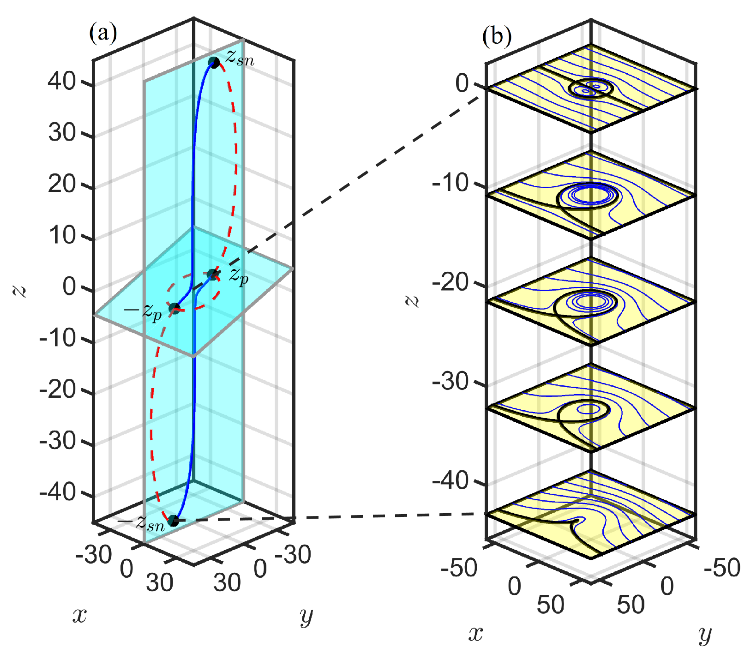
21) possess symmetries of translation in the horizontal plane and rotation about a vertical axis passing through the midpoint of the line connecting the vortices. Without loss of generality, therefore, we may align the vortex initial condition on the
y-axis, centered on the origin. Defining the vortex separation as
,
, gives the initial vortex positions as
and
, as depicted in
Figure 1.
In this configuration, the heton undergoes translation along the
x-axis with a velocity
and induces a velocity field given by
The dynamics simplify in a frame moving with the heton, i.e., we apply the change of variable
, under which the above equations of motion become autonomous:
The velocity field above is associated with a streamfunction
given by
One sees that the dynamics (
29) and (
30) are Hamiltonian, where
is the Hamiltonian and the horizontal positions of the passive scalars the canonical coordinates. This is a general feature of both 2D and QG hetons and reflects the fact that the fluid motion is 2D and incompressible.
The above equations of motion for passive scalars in the field of a 3D heton manifestly depend on three parameters, , Y, and Z. We choose units of time so that . One is also free to choose a unit of length. However, one cannot independently choose vertical and horizontal length scales as the ratio between these length scales has already been chosen to make the Brunt-Väisälä frequency . One possible scaling is to choose a length scale so that . This choice precludes investigating a heton with vertically aligned vortices, i.e., . Alternatively, one can choose a length scale so that , which precludes investigating a heton with vortices on the same horizontal plane, .
The dynamics of vertically aligned hetons,
, is relatively simple and rescaling does not provide additional insight. For horizontally offset hetons,
, we scale length and time such that
and
,
and drop primes. The resulting nondimensional equations of motion are:
The 3D dynamics are a function of a single parameter, the nondimensional vertical vortex half-separation
Z. For each vortex configuration with fixed
Z, the 3D dynamics foliate into independent 2D dynamical systems, parameterized by the height
z of the horizontal plane. Further, note that the nondimensional
Z obeys the relation
where the subscripts denote dimensional quantities. Typical values of
N and
f in the ocean at midlatitudes are
s
and
s
[
27], so
Z∼
corresponds to a heton with a dimensional aspect ratio of
∼
.
3. The Structure of Heton-Induced Transport
As a heton travels, it carries with it a trapped volume of fluid. Fluid within the trapped volume moves with the heton and rotates around the vortices as they move. Fluid outside this volume may be dragged along by the heton for a finite distance before ultimately being left behind.
As described in the above section, we work in a frame co-moving with the heton. In this co-moving frame, the trapped fluid has no net motion, and the untrapped fluid moves past the stationary heton with trajectories extending from infinitely far in front of the heton, where “front” refers to the direction in which the heton is heading, to infinitely far behind the heton. The heton is stationary in the co-moving frame and the trapped fluid rotates around the component vortices without leaving their neighborhood. In this co-moving frame, the trapped region is defined by the invariant stable and unstable manifolds associated with Equations (
26)–(
30).
These manifolds by definition belong to hyperbolic fixed points of the co-moving dynamics, and, since the system is Hamiltonian, they coincide with streamlines of the flow with the same value of as their associated fixed point. The structure of heton-induced transport is thus governed by the structure of the fixed points and their associated manifolds in the co-moving frame. It is useful to separately consider the three possible heton configurations: a vertically aligned heton with , (We can scale if we want); a horizontally aligned heton with , ; and the more general tilted heton with , .
3.1. Vertically Aligned Heton: ,
A vertically aligned heton,
,
, is stationary. The induced velocity field takes the form of axisymmetric rotation about the
z-axis. There are no fixed points in the velocity field and, thus, no manifolds. Since the heton is stationary and all trajectories rotate around the heton, the volume trapped by a vertically aligned heton is, in a sense, infinite. This has analogues in the two-layer case, as noted in [
12,
13].
3.2. Horizontally Aligned Heton: ,
For this case, the heton Equations (
32)–(
35) take the form:
Since, with , the equations remain unchanged under the transformation , the dynamics are symmetric about the plane .
At heights far above and below the heton, the heton-induced velocity is weak, the flow in the co-moving frame is dominated by the drift due to being in a moving frame, and there is no trapping (
Figure 2a). On the plane containing the vortices, the flow field contains four fixed points: two unstable saddles and two stable centers (
Figure 2b). As is typical for conservative systems, a separatrix connects the saddles and bounds the trapped region.
One can treat the height
z as a bifurcation parameter. As one moves up from
, the four fixed points are created by a double saddle-node bifurcation at some
and remain as one moves to
. As
z increases through zero and to
, symmetry shows that the fixed points disappear at
through another double saddle-node bifurcation. The bifurcation diagram is shown in
Figure 3a.
The location of the unstable fixed points can, for this case, be determined analytically. By symmetry, they occur at
. Then, (
37) gives
for all
x. Equating (
36) to zero along with the conditions
,
yields the fixed points
. The unstable fixed points are thus farthest apart in
x when
, i.e., in the plane containing the vortices, and the horizontal region trapped by the heton is thus largest on this plane. As one moves away from this plane, the trapping region shrinks, eventually disappearing altogether on the planes
at the double saddle-node bifurcations. Requiring that the
x-coordinate of the fixed point be real shows that the saddle-node bifurcation occurs at
. The stable fixed points are determined by repeating the process above with
. Again,
vanishes. The equation for the zeroes of
now, however, must be found numerically.
The three-dimensional volume trapped by the heton can be inferred from the contour slices seen in
Figure 3b. The case under consideration here,
,
, has no remaining free parameters. The trapped volume is therefore a finite constant. Reversing the non-dimensionalization (
31) reveals that the volume of trapped fluid scales as
, the cube of the horizontal half-separation between the component vortices of the heton.
3.3. Tilted Heton: ,
The most general case, a tilted heton with
and
, is described by Equations (
32)–(
35). Tilting the heton breaks the symmetry in
z and the dynamics differ across the
plane. However, Equations (
32)–(
35) do remain unchanged under the transformation
We note that a more physical version of this symmetry is to keep time moving forward but change the signs of the vortex circulations. This “mirror” symmetry is useful in simplifying the analysis.
The phase portraits now show three different structures (
Figure 4). Again, far above and below the heton,
and
, the heton-induced velocity is small, the flow is dominated by the drift, and there are no fixed points and no trapping (
Figure 4a).
Again, treating
z as a bifurcation parameter and moving up from
, we start with no fixed points. We then reach a range of
z with two fixed points, one stable and one unstable, with a trapping region bounded by a homoclinic connection (
Figure 4b). As
z moves closer to zero, we find a range of heights with a structure similar to that previously seen when
. This region has two stable centers, two unstable saddles, and a trapping region bounded by heteroclinic manifolds. Unlike the
case, the phase portrait is only symmetric in
y when
. For each height where a trapping region exists, the trapping region is bounded by the contour
, where the subscript denotes the streamfunction value at the unstable fixed point at the height
z.
The bifurcation diagrams for
(
Figure 5a and
Figure 6a) show the bifurcation sequence. As one moves up from
, there is saddle-node bifurcation at
, which is now a function of
Z, creating a single stable center and a single unstable saddle with a homoclinic connection bounding the trapping region. As one moves up from
, there is a second bifurcation, a pitchfork bifurcation, at
, where the unstable fixed point changes stability to become a stable center and creates two new unstable saddles with a heteroclinic connection. The centers invariably lie on the
y-axis, as in the
case. The saddles, which had
for all
z when
, now have
for
. Increasing
z through zero to
reverses the bifurcation sequence, with a subcritical pitchfork bifurcation at
and a saddle-node bifurcation at
.
The 3D fluid surrounding each tilted heton thus has three distinct dynamical regimes depending on the height z in the fluid relative to the heton center plane:
A heteroclinic regime, . This regime is characterized by the presence of four fixed points, two stable and two unstable. The unstable fixed points are connected by heteroclinic orbits, which bound the trapping region in each horizontal plane.
A homoclinic regime, . This regime is characterized by the presence of two fixed points, one stable and one unstable. The unstable fixed point has an associated homoclinic orbit, which bounds the trapping region in each horizontal plane.
A drift regime, . This regime has no fixed points and no trapping.
The unstable fixed points in the heteroclinic regime can be found analytically by setting the expressions (
32) and (
33) to zero for nonzero values of
x. This produces the roots
These roots are real when
and thus the pithfork bifurcation occurs at
independent of
Z. We note that this is the same height as the saddle-node bifurcation when
, i.e.,
. The other fixed points are not amenable to analytical discovery, and must be computed numerically (see
Figure 5a and
Figure 6a).
4. Volume Trapped by a Tilted Heton,
The fixed points and manifolds in a tilted heton, and therefore the volume
of its trapping region, depend on the heton’s vertical half-separation
Z. The contour slices of
Figure 5b and
Figure 6b roughly illustrate the shape of the 3D trapped volume, as well as its growth size as
Z increases. Here, we propose a scaling theory for the trapped volume
for
and compare it with numerical computations.
4.1. Scaling Theory for
The trapped volume is defined by the interplay between two parts of the streamfunction (). The first two terms in () are contributions from the component vortices of the heton,
, where
is the distance from the position
of a passive particle to the vortex with circulation
. These vortex contributions are denoted
. The third term is a drift term due to being in a co-moving frame,
Writing the streamfunction as , we build a scaling theory for from three assumptions:
The scaling of the streamfunction determines the scaling of the trapped volume;
The vortex and drift components of the streamfunction scale uniformly, ∼;
The scaling is isotropic, ∼ with .
The first assumption is motivated by the fact that the manifolds of the streamfunction determine the trapped volume. The trapped volume should thus scale with the streamfunction. The second assumption is based on the idea that the boundary of the trapped volume is the crossover region where drift and vortex-induced velocities balance each other. We thus expect ∼ for the streamfunction values on the manifolds. The final assumption, isotropic scaling, is a reasonable simplification, although, as QG dynamics are anisotropic between the horizontal and vertical, anisotropic scaling would not be unphysical.
We define nondimensional scaled coordinates
, and then drop the primes. The drift term in scaled coordinates is
The squared distance from the vortex is
where
. The largest term in
, i.e., the term with the largest exponent on
Z, depends on the value of
. Define the largest term as
. Then
The total squared distance can be written as
, where
is obtained from Equations (
42) and (
43) by
. Expanding
gives
and then
For , and the leading-order contribution to is given by ∼∼. In this case, , ∼, and thus the assumption that ∼ cannot be satisfied, , is inconsistent with the scaling theory.
When
or
,
, and the leading-order term in
is given by the leading-order term in
,
For the case , ∼ requires , which has no solutions. Thus, is also inconsistent with the theory. The final case, , leads to , which has one solution , and is consistent with the requirement for the case being considered. Thus, isotropic scaling theory leads to a single scaling exponent, . Then, ∼ and ∼∼. The dimensional trapped volume then scales .
4.2. Numerical Calculation of the Trapped Volume
We have already seen that for vertically aligned hetons,
, the trapped volume is, in some sense, infinite. The trapped volume in the remaining two cases, defined by
and a single value of
Z, can be calculated numerically. The trapped region is bounded by the invariant manifolds of the unstable fixed points. These manifolds are streamlines with streamfunction
, where
is the value of the streamfunction at the associated unstable fixed point at height
z. The values of
relative to
in the homoclinic and heteroclinic regimes are shown in
Figure 7.
To calculate the trapped volume
, we numerically solve (
32) and (
33) for the unstable fixed points over a range of
z from
, where we know the fixed points exist, to
, where the fixed points have vanished and no fluid is trapped. At each value of
z, we calculate
from (
34) and demarcate the trapped region using the geometry in
Figure 7. The trapped area bounded by
is then found by numerical integration. Further numerical integration of the trapped area over the heights where trapped fluid exists gives the trapped volume. Solving for the fixed points requires balancing two numerically calculated terms. As
Z becomes large, these terms become large and numerical error limits the accuracy of the solution. As a result, we restrict our calculation of the trapped volume to the range
.
The height of the saddle-node bifurcation
and the trapped volume
are shown in
Figure 8. We see that the scaling theory is approximately verified, with the growth slightly shallower than the scaling theory predicts. We conjecture that at larger
Z, the scaling theory becomes more accurate.
5. Discussion
Since their inception in the papers by Gryanik [
11,
23] and Hogg and Stommel [
12], point vortex hetons have been used to model a variety of geophysical transport phenomena. Central to these studies is the fact that a moving heton carries with it a finite volume of fluid. In this paper, we have characterized the volume trapped by a single 3D heton in an infinite, continuously stratified fluid with no background flow and constant Coriolis and Brunt-Väisälä frequencies.
A heton is fully defined by the 3D position of each vortex and their common circulation. Translational symmetry in space and time, horizontal isotropy, and the choice of a length scale allow all hetons to be characterized by vortex separation alone. The 3D fluid dynamics of each heton configuration foliate into a family of 2D horizontal Hamiltonian systems parametrically dependent on the heton configuration parameter and the vertical distance in the fluid from the center of the heton.
The possible heton configurations separate into three categories with distinct transport properties. Vertically aligned hetons have zero horizontal separations and are all similar as the vertical separation can be scaled to unity. They are stationary and induce axisymmetric rotation about the z-axis. Since there is no translation of fluid relative to the heton, there is no long-range transport and we might say that the trapped volume is infinite. The remaining two configurations have well-defined three-dimensional trapping regions. Horizontally aligned hetons have vortices with zero vertical separation and are also all similar as the horizontal half-separation Y can be scaled to unity. Horizontally aligned hetons exhibit trapping in the region of the fluid where the dimensional height z satisfies . The trapping region is bound in each horizontal plane by a heteroclinic separatrix symmetric across the line bisecting the vortex separation. The more general tilted hetons, whose vortices have nonzero horizontal and vertical separations, are characterized by a single parameter, the ratio of the vertical half-separation to the horizontal half-separation, . These hetons exhibit a trapping region that is bounded by heteroclinic separatrices for regions of the fluid with dimensional height , where a pitchfork bifucation occurs, and by homoclinic separatrices when , where is the height were a saddle-node bifurcation occurs. From scaling theory and numerical simulations, we find the dimensional trapped volume scales as for .
Two common idealizations of fluid stratification are the 3D uniform stratification studied here and a two-layer QG fluid. Transport by two-layer hetons shows some analogues with the results found here [
12,
13]. Two-layer hetons are characterized by a single parameter, the ratio between the horizontal vortex separation and the interfacial Rossby radius. Young [
13] showed that when the vortices are both in the upper layer, there is always trapped volume in the upper layer and trapped volume in the lower layer only when the separation parameter is below a threshold. This is analogous to our horizontally aligned heton, where the trapped volume extends a finite height above and below the plane containing the heton. The two-layer analogue of our tilted heton is a heton with one vortex in each layer. Young [
13] showed that every such heton is in either a homoclinic or heteroclinic regime depending on the horizontal vortex separation. This single regime fills the entire fluid with streamfunctions in the two layers being the opposite of each other,
. This differs from the 3D heton studied here in that we find that every tilted heton configuration has all three regions described above. In the two-layer tilted heton analogue, one can never experience a height without a vortex, and hence the entire fluid displays trapping. In the 3D case, the trapped volume grows without bound as the vertical vortex separation grows with fixed horizontal separation. This behavior has an analogue in the two-layer case, where the trapped volume grows without bound as the horizontal separation decreases [
12,
13].
Our analysis of the idealized model presented here reveals that the trapped region in the QG heton is trapped forever and that the region is defined by the heteroclinic/homoclinic connections in the phase space of the Hamiltonian. If the Hamiltonian is perturbed, it becomes possible for these connections to break, leading to Lagrangian chaos and a region with finite time trapping and Lévy flights [
28,
29], i.e., systematic perturbation of the Hamiltonian may allow access to dynamics more closely approaching real-world phenomena. One physically interesting perturbation is the inclusion of ageostrophic effects, which bring in small-order Rossby number corrections, including a small, nonzero, vertical velocity. A recently developed theory for ageostrophic 3D point vortices [
30] will allow the study of ageostrophic perturbations to hetons and may show finite time trapping and Lévy flights. Further, oceanic motions typically have a non-zero background flow component. Previous studies of the interaction of background flows with two-point-vortex systems in the two-layer case [
6] and the continuously stratified case [
25] suggest the possibility of relative motion between the constituents of the heton, inducing as a result chaotic passive particle trajectories. Finally, on very large spatial scales, the Coriolis frequency is no longer constant, and the so-called
-effect needs to be taken into account. Point-vortices on the
-plane display richer dynamics than those on the
f-plane, including the ability to self-advect [
6] and radiate Rossby waves [
14]. A systematic study of these and other interesting perturbations—a fluid with more point vortices than a single heton, a generalization of the point-vortex heton to hetons with distributed vortices—is left to future work.


