Abstract
This work presents a multi-node lumped parameter model able to predict the steady and transient behavior of capillary heat pipes, taking into account the effects of gravity (orientation angle) and the real gas effects in the vapor modeling. The model was validated against experimental results acquired by Leonardo S.p.A., which were obtained by simulating the behavior of a heat pipe embedded in a chassis cover, subject to seven cycles of transient thermal loading. After the validation, the analysis is focused on the model accuracy when using the ideal and real gas assumptions, using different working fluids (water, ammonia, acetone, HFC134a). The results showed that when using water or ammonia as working fluid, the error in modeling the vapor as an ideal instead of as real gas is negligible, both for the vapor temperatures and pressures predictions. On the contrary, when using acetone or HFC134a as working fluid, modeling the vapor as a real gas leads to a significant increase in the accuracy of the vapor pressure predictions.
1. Introduction and State of the Art
Heat pipes (HP) are very attractive components in the area of spacecraft cooling and temperature stabilization due to their low weight penalty, very low maintenance, and high reliability [1]. Nowadays, heat pipes have been studied for more than fifty years, and they are one of the most popular passive thermal control devices for many engineering fields.
The structure of a heat pipe consists of a sealed system containing a fluid, the so-called working fluid, which cyclically evaporates and condenses. Through the evaporation process, the working fluid removes heat from the component to cool down. This thermal power removed is dissipated into the external environment by means of the condensation process. Therefore, the heat pipe is a device with very high thermal conductivity that enables the transportation of heat whilst maintaining almost uniform temperature along its heated and cooled sections [2]. This means that it works in nearly isothermal conditions.
The capillary driven heat pipe (CHP) is the most commonly used and known type of heat pipe. In fact, it is used in many industrial applications, such as computer cooling [3] and spacecraft thermal control [1]. This type of heat pipe consists of a sealed container, whose inner surface is covered with a porous structure, the wick. The container is partially filled with a working fluid [4]. One end of the container, the evaporator, is heated by a heat source. Thus, the working fluid evaporates, and the vapor moves to the other end of the HP, the condenser, possibly passing through an adiabatic zone. The condenser area is cooled so that the vapor can condense. The function of the wick material on the inner surface of the heat pipe is to guide the condensate back to the evaporator [4]. This process occurs mainly because of the action of capillary forces. However, gravitational force can have a great influence on the behavior of the CHP. In fact, its presence can make the HP operation orientation-dependent, and only a proper design of the wick can allow the HP to operate in all directions and to reach the requested performance [3]. The material composing the wick must be compatible with the working fluid, in order to avoid undesired effects, such as corrosion or generation of non-condensable gas. For this reason, the most common wick/fluid couplings are: copper/water, mainly used for electronics applications; aluminum/ammonia, and aluminum/acetone, mainly used for spacecraft applications; copper/HFC134a refrigerant, mainly used for energy recovery applications.
In the past decades, there have been many attempts to model the different types of heat pipes.
A possible way to model both the steady-state and transient behavior of a loop heat pipe was described by Cullimore and Baumann [5]. This is done by using the NASA-standard thermohydraulic analyzer, SINDA/FLUINT, to design and simulate thermal/fluid systems that can be represented in networks corresponding to finite difference, finite element, and/or lumped parameter equations. The only disadvantage of this model is that it requires a good knowledge of loop heat pipe operation and of the thermophysical processes involved in those devices, at least for detailed studies.
A transient model for microgrooved heat pipes by using a macroscopic approach was presented by Suman et al. [6]. This model was developed by using an equilateral triangular heat pipe as test case, but the equations are suitable to be used with heat pipes of any polygonal shape. The flow is modeled as unsteady, incompressible, and one-dimensional along the length of the heat pipe. The coupled non-linear governing equations of heat, mass, and momentum transfer are simultaneously solved to obtain the transient and steady-state profiles of the main parameters which characterize the heat pipe behavior (temperature, pressure, flow velocity). However, this model can be used only for microgrooved heat pipes with a polygonal shape.
A lumped parameter model for capillary heat pipes was developed by Ferrandi et al. [7,8]. This model, based on the electrical analogy, divides the heat pipe in two parts, the solid network and the fluidic network, that are connected by coupling equations. The model considers the vapor as an ideal gas and it does not take into account the influence of gravity (and therefore of the orientation angle) on the heat pipe behavior.
Another lumped parameter model for loop heat pipes was developed by Bernagozzi et al. [9]. As the previous one, this model is based on the electrical analogy and it does not consider the real gas effects in the vapor modeling and the gravity effects.
A model able to predict the heat transfer performances of a closed vertical meandered pulsating heat pipe, filled with water, was proposed by Wang et al. [10], and it is based on artificial neural networks. This model can be used to predict the thermal resistance of the pulsating heat pipe, given filling ratio and related geometric parameters, at different heat fluxes. The analysis showed a good agreement between numerical and experimental results. However, in order to use artificial neural networks for predicting the pulsating heat pipe behavior, some other studies with different working fluids and more experimental data are necessary.
A simple model able to predict the thermal performance and working temperature of a multi-channel flat plate heat pipe was developed by Guichet et al. [11], and it includes the cooling manifold to estimate the characteristics of the complete system. However, this model was developed only for a very specific type of heat pipe, so it could be difficult to use in different applications.
An advanced conduction-based heat pipe model was recently developed by Zimmermann et al. [12]. An analytic expression to calculate the pressure drop inside the vapor core was developed, and the results were validated through CFD simulations. This model is quite easy to implement and it showed good results, but it is designed for steady conditions. Thus, there is no evidence that it also works in transient conditions.
The aim of this work is to build and validate a simple, multinode, lumped parameter model, which is able to predict the steady and transient behavior of capillary heat pipes, including the gravity (orientation angle) effects and the real gas effects in the vapor modeling. The model was built to be quite versatile, in fact, it can be used for heat pipes of every possible shape and geometry that can be described and/or modeled analytically, as well as for all the solid–fluid couples whose thermophysical properties are known. The model was validated by using a real dataset provided by the company Leonardo S.p.A., referring to an experiment performed by using a flat heat pipe made of copper and filled with water as working fluid. After the validation, the model was used for predicting the heat pipe behavior, when four different solid–fluid couples are used (copper–water, aluminum–ammonia, aluminum–acetone, copper–HFC134a refrigerant). A specific focus is placed on assessing for which fluids and working conditions the ideal gas assumption grants a good accuracy, and for which ones, on the contrary, its use is not suitable, and real gas properties must be included in the model.
2. Heat Pipe Model Description
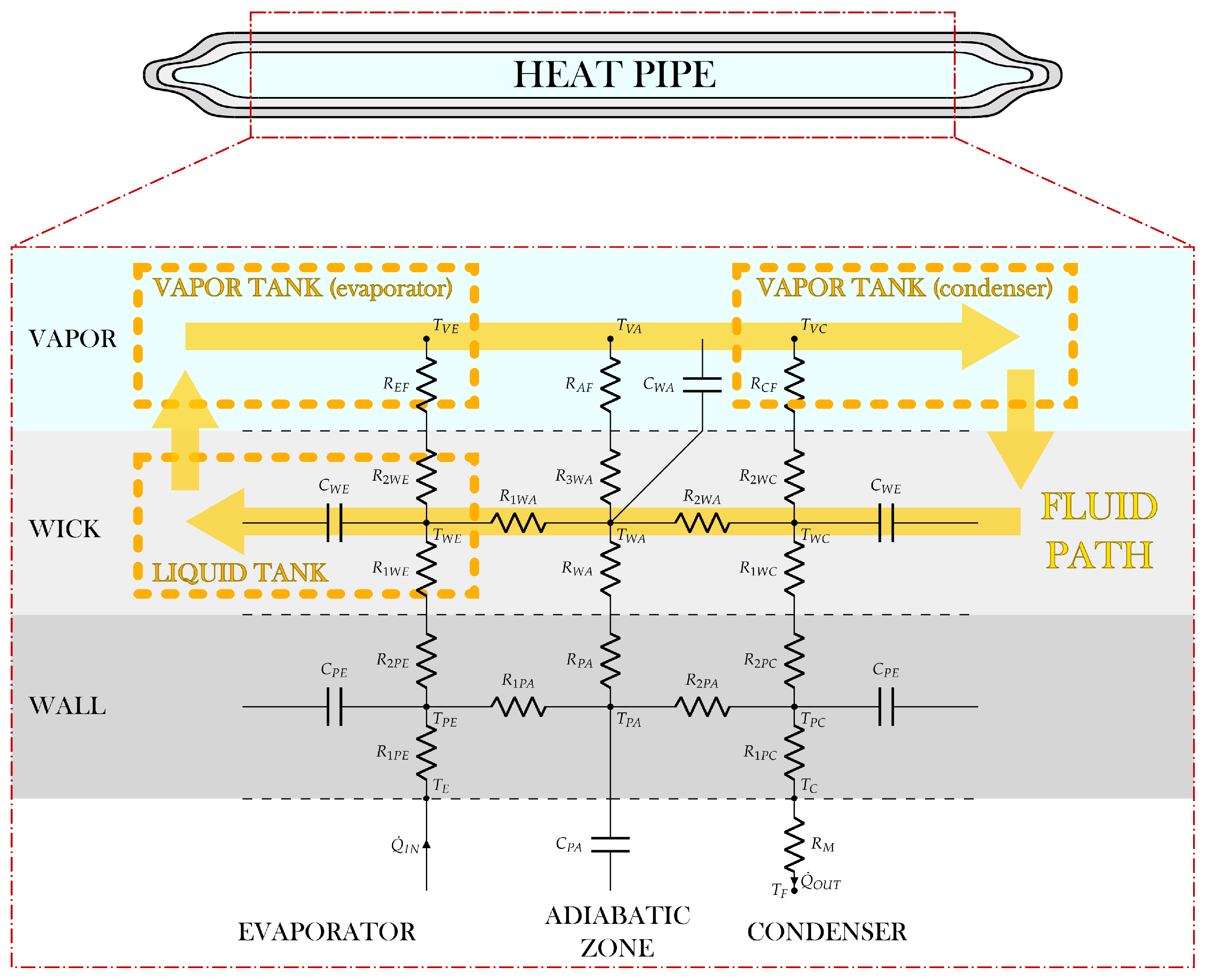
Figure 1 shows the conceptual model of the heat pipe used in this work. To use the lumped parameter approach, the heat pipe scheme can be conceptually divided into two major parts, the solid network and the fluid network, as in [7,8,9]. Each of these networks can be further divided into different minor parts, called nodes or lumps. Each node represents a section of the complete heat pipe, and all its thermophysical properties are considered uniform across the whole section, and equal to their average value in the section, which is assumed to be the one at the center of the volume of the node which represents the considered section (midpoint rule).
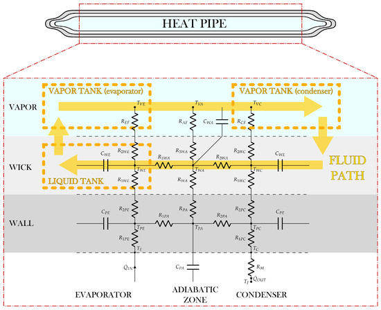
Figure 1.
Heat pipe scheme.
The solid network is modeled through the use of the electrical analogy, in which the currents are represented by the heat transfer rates, and the voltages are represented by the temperature differences between two nodes. All the nodes are connected to the adjacent ones, to the fluid network, and to the external environment through thermal equivalent resistors and capacitors.
Since the fluid network must also take into account the presence of gravitational terms, it cannot be modeled by the electrical analogy, because it is not a passive network as it would have been without gravitational forces. Therefore, this part of the system is modeled through the one-dimensional Navier–Stokes equations and the equations of real gases.
Then, the coupling between the solid and fluid networks, and the one between the liquid and the vapor must be considered in order to obtain the complete set of equations describing the behavior of the entire heat pipe.
2.1. Solid Network
The scheme of the solid network is represented in Figure 1, where dashed lines separate the vapor zone, wick, solid wall, and external regions (evaporator and condenser).
The solid network is modeled using a total of six nodes, three in the solid wall (, , ), and three in the wick (, , ). For both the wall and the wick, there is a node representing the evaporator section (subscript E), a node representing the adiabatic section (subscript A), and a node representing the condenser section (subscript C). These nodes are connected to three nodes in the vapor zone (, , ), which belongs to the fluid network, and to two nodes on the external walls, namely, at the evaporator, at the condenser. The latter is in its turn connected to a node representing the external environment ().
In Figure 1, the symbol T represents the temperature of a node, the symbol represents a heat power, which can be the one entering the system from the evaporator wall, , or the one exiting the system from the condenser wall, . The symbol R represents the resistance of a thermal equivalent resistor, and the symbol C represents the capacitance of a thermal equivalent condenser. The resistances in the solid wall and in the wick are conductive, the ones connecting the wick to the vapor zone are convective, and the one connecting the condenser wall to the external environment is mixed, which means that it can be conductive, convective, radiative, or a combination, depending on the boundary conditions of the specific case.
The resistances , , , and are axial, in fact, they model what happens along the longitudinal dimension of the heat pipe, namely, from the evaporator to the condenser. Conversely, all the other resistances are radial, describing the thermal behavior along the radial direction of the heat pipe, namely, from the center of the vapor zone to the solid wall.
The resistance and capacitance of each branch of the network depend on the geometry of the heat pipe section. Therefore, the equations used to describe them will be analyzed in Section 3, where the geometry of the case study is described.
At this point, writing an energy balance on each solid node, it is possible to draw six equilibrium equations.
For the evaporator wall node, the equilibrium equation is:
where is time. In Equation (1), either the input thermal power, , or the evaporator wall temperature, , has to be known. In this second case, the input thermal power to be used in Equation (1) is:
For the condenser wall node, the equilibrium equation is:
In Equation (3), either the output thermal power, , or the external environment temperature, , has to be known. As before, in this second case, the output thermal power to be used in Equation (3) is:
For the adiabatic wall node, the equilibrium equation is:
For the three wick nodes (evaporator, condenser, and adiabatic zone), the equilibrium equations are respectively:
The vapor temperature in the evaporator zone, , in Equation (6), and the vapor temperature in the condenser zone, , in Equation (7), are taken from the fluid network. Moreover, in Equation (8), the vapor temperature in the adiabatic zone, , has to be known. It is computed as a weighted average of temperatures and , as shown in System (9):
where , , and are the evaporator, adiabatic zone, and condenser lengths, respectively; is the effective duct length (), and are the weights that take into account the fact that the center of the adiabatic zone can be closer to the condenser than to the evaporator, or vice versa.
2.2. Fluid Network
In order to write the equations which describe the fluid network, six assumptions are necessary. It is assumed that:
- the fluid flow is one-dimensional and laminar for both phases;
- vapor transformations in the evaporator/condenser tanks are isoentropic;
- evaporation and condensation only occur in the evaporator and condenser zones, therefore, the mass flow rates of the phases do not change in the adiabatic region;
- the liquid temperature is exactly equal to the wick temperature for each point along the wick length;
- the thermophysical properties of the liquid, the surface tension, and the latent heat of vaporization are evaluated in saturation conditions;
- All the condensing fluid reaches the wick, with no “accumulation” before it.
With reference to Figure 1, heat enters the fluid network arriving from the external heat source into the evaporator liquid tank, so that the working fluid in liquid state evaporates and conceptually flows into the vapor tank, thanks to the capillary pressure jump. Then, the vapor formed flows through the adiabatic vapor duct and arrives to the condenser vapor tank, from which a certain quantity of heat is removed. This phenomenon causes the vapor to condense and flow back to the evaporator, where the cycle restarts.
At this point, it is possible to analyze each piece of the fluid network, and to write the equations which describe its behavior. In such equations, the mass flow rate of the vapor is indicated with , the one of the liquid is indicated with , the one that evaporates is indicated with , and the one that condenses is indicated with .
2.2.1. Condensed Liquid
For the last assumption in Section 2.2, it is possible to state that:
Equation (10) highlights the fact that there is no accumulation of liquid in the condenser.
It represents the first of the nine equations for the fluid network.
2.2.2. Vapor Tanks
In order to write the equations that link the vapor pressures and mass flow rates, it is necessary to start from the continuity equation. For the vapor, it can be written as:
where is the volume of the vapor tank considered, is the vapor density, are the N vapor mass flow rates crossing the tank boundaries (taken as positive when entering). However, it is possible to write the vapor density derivative with respect to time as a function of the vapor pressure , as:
For the second assumption in Section 2.2, the vapor in the tanks undergoes isoentropic expansion or compression. In isoentropic conditions, it is possible to state that:
where is the speed of sound in the vapor at the current temperature and pressure. Therefore, substituting Equation (13) in Equation (12), we obtain the two equations which link the vapor pressures and mass flow rates, from the point of view of the evaporator and condenser tanks, respectively:
where and are the vapor pressures in the evaporator and condenser zones, respectively; and are the volumes of the evaporator vapor tank and condenser vapor tank, respectively; and are the sound speeds in the vapor in the evaporator and condenser zones, respectively.
The two equations in System (14) must be added to the complete set of equations for the fluid network.
2.2.3. Vapor Pressure–Temperature Relation
The general relation between the vapor temperature and pressure is not trivial. However, since the considered vapor transformations are isoentropic, it is possible to write the entropy differential, , as a function of T and p, and to impose this differential equal to zero. In particular [13]:
where is the specific heat at constant pressure of the considered gas, and is the isobaric expansion coefficient. Imposing the entropy differential equal to zero, dividing Equation (15) by the time differential, , and referring the terms of Equation (15) to the vapor in the evaporator and condenser, one obtains:
where and are the vapor isobaric expansion coefficients in the evaporator and condenser zones, respectively; and are the vapor densities in the evaporator and condenser zones, respectively; and are the vapor specific heats at constant pressure in the evaporator and condenser zones, respectively.
The two equations of System (16) are two of the nine equations that must be added to the complete set for the fluid network.
2.2.4. Evaporation and Condensation
Since the evaporation and condensation phenomena are lumped in the evaporator and condenser zones, for the third assumption in Section 2.2, the mass flow rates which evaporate and condense can be computed as:
where is the thermal power going from node to node , namely, the effective thermal power used for evaporation; is the thermal power going from node to node , namely, the effective thermal power extracted for condensation; is the latent heat of vaporization computed at an intermediate temperature between and ; and is the latent heat of vaporization computed at an intermediate temperature between and .
The equations of System (17) have to be added to the complete set of equations for the fluid network.
2.2.5. Vapor Line
Considering the vapor line, it is possible to write the one-dimensional and laminar form of the Navier–Stokes equations describing the conservation of momentum, as:
where u is the vapor velocity, g is the gravity acceleration, is the vapor dynamic viscosity, and is the heat pipe orientation angle. In particular, can range between −90° and 90°: it is equal to 0° when the heat pipe is oriented horizontally; it is negative when the evaporator is above the condenser; it is positive when the evaporator is under the condenser. In most cases, this last condition is the most favorable for heat pipe operation because gravity helps the liquid to flow from the condenser to the evaporator. Conversely, when is negative, the liquid pressure in the condenser must be high enough to compensate the gravity pushing the liquid back to the condenser zone.
Equation (18) can be integrated over the effective duct length, , as:
Starting with the time derivative term, it is possible to write (using the relation in the last step):
where is the vapor velocity, is the vapor density in the adiabatic section, and is the cross-sectional area of the vapor duct.
As the flow is assumed as laminar (first assumption), the second term of Equation (19) can be rewritten as:
where is the hydraulic diameter of the vapor duct, is the vapor dynamic viscosity in the adiabatic section, and is the Reynolds number ().
The third term of Equation (19) can be rewritten as:
Finally, the last term of Equation (19) can be rewritten as:
Therefore, the equation for the vapor line to be added in the complete set of equations for the fluid network is:
Equation (24) expresses the relation between the vapor mass flow rate, the pressures in the vapor tanks, and the gravitational contribution.
2.2.6. Liquid Line
Analyzing the liquid line, first of all, it is possible to write the liquid mass flow rate as a function of the wick porosity , that is, the liquid fraction capability of the wick, namely, the ratio between the volume of voids in the wick and its total volume:
where is the liquid velocity; is the liquid density in the adiabatic zone; and is the cross-sectional area of the wick.
Next, the pressure drop in a porous medium can be expressed through Darcy’s law [14]:
where is the velocity in the x direction, is the dynamic viscosity, is the body force in the x direction, and K is the wick permeability, which can be estimated by using the Blake–Kozeny equation [15,16]:
where is the pore radius. Consequently, the equation describing the liquid line can be written as
2.3. Solid–Fluid Coupling
The solid–fluid coupling is described by four equations. The first two equations describe the coupling between the wick temperature and the liquid temperature, which, given the forth assumption in Section 2.2 are always equal, so that the equations read:
where and are the liquid temperatures in the evaporator and condenser zones, respectively.
The other two equations for the solid–fluid coupling are those that define the heat transfer rates and , as functions of some temperatures and resistances, which are taken from both the solid and fluid networks. In particular, by looking at Figure 1, it is possible to state that:
The two equations of System (30) describe the mathematical expression of the heat transfer rates that is necessary to give () or extract () from the fluid, in order to make it evaporate or condense.
2.4. Liquid–Vapor Coupling
The liquid–vapor coupling is described by only one equation, namely, the Laplace–Young equation [17]. It describes the capillary pressure jump in the evaporator as a function of the liquid surface tension at the evaporator temperature, , the contact angle, , and the capillary radius, , as:
In Equation (31), the contact angle is assumed to be constant during the operation (neglecting contact angle hysteresis), but dependent on the fluid–solid couple, while the effective capillary radius, , is computed as a function of the pore radius, , as [8]:
Equation (31) is the last one to be taken into account for the description of the complete model.
2.5. Implementation of the Complete Set
From the previous sections, it is possible to conclude that the heat pipe behavior is described by twenty equations, namely, eleven ordinary differential equations and nine algebraic equations, which contain twenty unknowns. Therefore, the system is fully determined.
The equations are:
The unknowns can be classified as:
- Ten temperatures: ;
- Four pressures: ;
- Four mass flow rates: ;
- Two heat transfer rates: .
In order to solve System (33), an explicit method is used. In particular, the eleven differential equations are discretized by the forward finite differences approach and solved for each time step. Then, the remaining nine algebraic equations are sequentially solved.
Since the forward finite differences approach is an explicit method, and since the number of equations to be solved is quite large, the stability of the solution requires a very low time step. However, this does not greatly affect the computational time, which remains absolutely manageable.
In the solution process, the thermophysical properties of the liquid (saturation pressure, density, viscosity, thermal conductivity), the surface tension, and the latent heat of vaporization are evaluated by using a polynomial interpolation of the saturation table of the working fluid (fifth assumption in Section 2.2). Conversely, the thermophysical properties of the vapor (density, viscosity, specific heat at constant pressure, isobaric expansion coefficient, sound speed) are evaluated at the current temperature and pressure, with the aid of some look-up tables. Such tables were created using the REFPROP software (version 9.1), from the National Institute of Standards and Technology [18]. The data contained in these tables are extracted with a nearest neighbor approach, in order to obtain meaningful results also near saturation conditions.
Further details about the numerical implementation method can be found in Appendix A.
3. Case Study
As already said, the model was first of all validated against experimental results acquired by Leonardo S.p.A. The heat pipe used for the experimental test is shown in Figure 2a. It is a copper heat pipe using water as the working fluid. In order to be easily brazed to the aluminum chassis, the HP was covered by a very thin electrolytic nickel plate (thickness ).
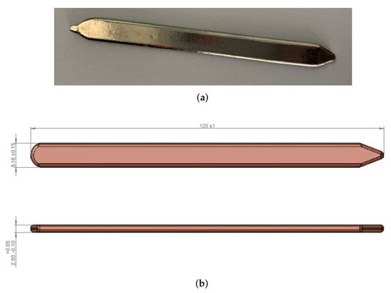
Figure 2.
Picture and dimensions of the heat pipe used in the experimental test (a) Heat pipe picture. (b) Heat pipe dimensions.
The external dimensions of the HP are shown in Figure 2b. It is worth mentioning that since the two ends of the heat pipe are not straight, but sharpened, the total length that will be given as an input to the model is not , but , in order to compensate for the loss of thermal exchange area due to the sharpening.
From Figure 2b, it is also possible to notice that the section of the HP is not cylindrical. In fact, the thickness is much lower than the width. Concerning the internal dimensions:
- The thickness of the wall is equal to ;
- The thickness of the wick is equal to ;
- The wick porosity, , is approximately equal to ;
- The average grain radius is approximately equal to 100 μm.
3.1. Description of the Experiment
In the experimental test, three heat pipes like the one shown in Figure 2 were embedded in a chassis cover made of the aluminum alloy 6082, as shown in Figure 3. In particular, the empty chassis with the three cavities can be seen in Figure 3a, the heat pipe ready to be embedded in a cavity can be seen in Figure 3b.
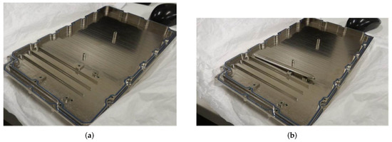
Figure 3.
Test device (a) Aluminum chassis. (b) Heat pipe embedding.
After the heat pipe embedding, a (Ohmite Manufacturing Company) resistor was placed on the evaporator zones of the three heat pipes, to be used as thermal source. The resistor was fixed with a bracket to ensure mechanical and thermal contact of the power component.
Then, the front face of the chassis was entirely blackened, in order to perform a proper measurement by using an infrared thermocamera, and two thermocouples were placed on the two opposite sides of the central heat pipe.
Given the placing of the setup, it is possible to state that the heat pipes have a vertical bottom-heating orientation, with the condenser over the evaporator. Therefore, the orientation angle to be used in the model is equal to 90°.
Furthermore, the heat pipe condenser zone is able to exchange thermal power by conduction with the chassis cover, by natural convection with the air, and by radiation with the room walls. Thus, the resistance connecting the condenser external wall and the external environment, , is a mixed resistance.
The experiment was performed by turning on the resistor for , then turning it off for , and repeating the same cycle of thermal charge and discharge six more times, for a total of seven cycles, and a total time of .
The total thermal power given by the resistor in the thermal charge phases is , but only a part of it is taken by the heat pipes. In fact, a great part is directly dissipated by the chassis cover to the external environment.
The results of this experiment, namely, the temperatures acquired by the thermocouples, are the output to be compared with that from the model object of this study. However, before this step, it is necessary to adapt the latter to the geometry of the real heat pipe, and to extract the data of and to be given to the model as input parameters.
3.2. Model Adaptation
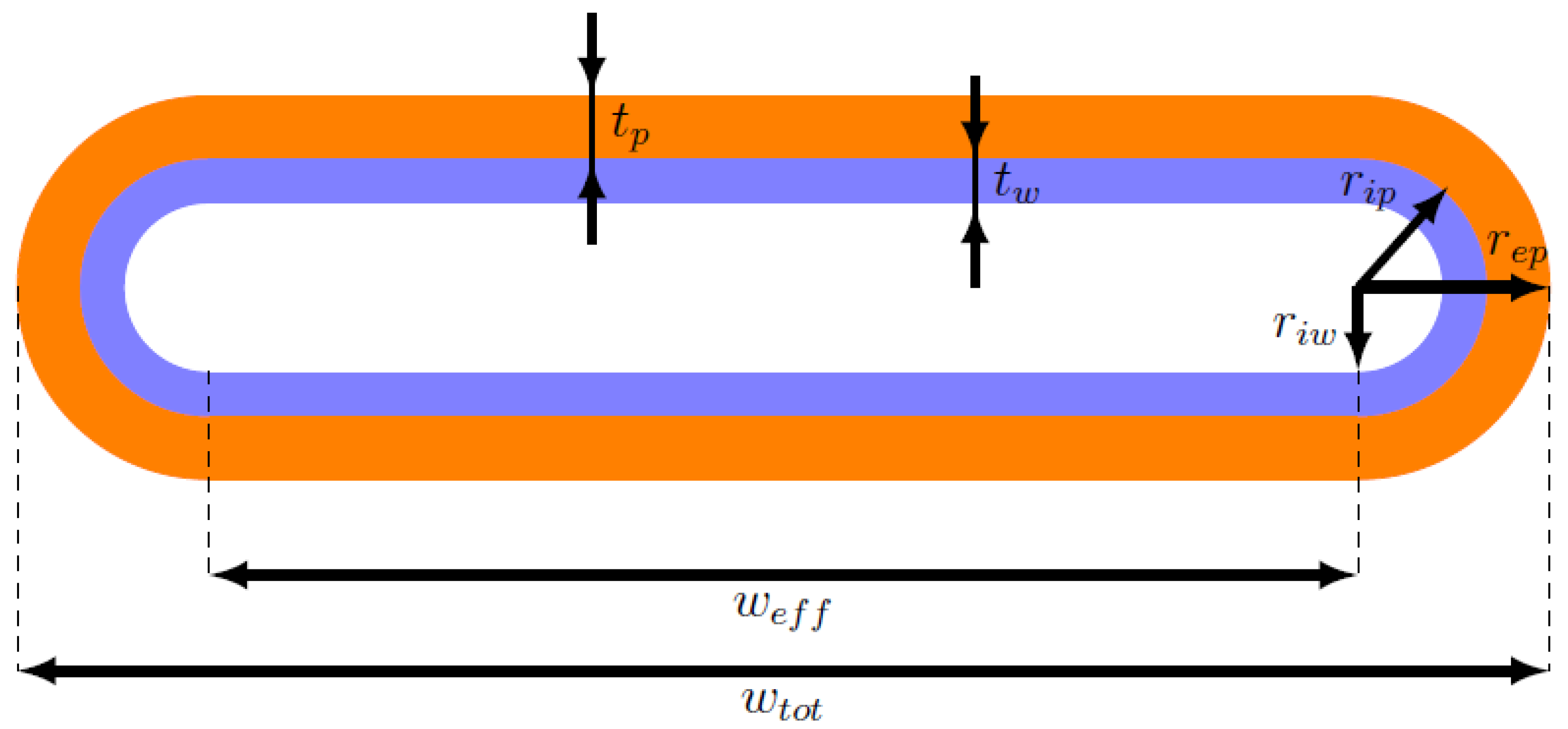
For the aim of this work, the shape of the heat pipe cross-section can be modeled as a rectangle with two semicircles at the two ends, as can be seen in Figure 4. Therefore, the formulas used for computing the resistances and capacitances of the solid network, and the formulas for the quantities multiplying , , and in the fluid network equations must be adapted to this geometry.
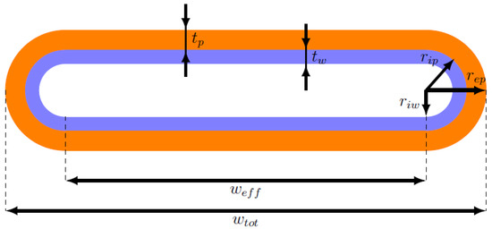
Figure 4.
Scheme of the real heat pipe section.
First, it is useful to define the cross-sectional areas of the wall, , wick, , and vapor zone, , in the new domain:
where:
- , , and are the external wall, internal wall, and internal wick radii of the circular regions at the ends of the section, respectively;
- is the effective width of the section, which corresponds to the total width minus twice the external wall radius: ;
- is the wall thickness: ;
- is the wick thickness: .
At this point, it is possible to define all the aforementioned quantities in this specific domain.
3.2.1. Solid Network
For the capacitances of the solid network, the adaptation is straightforward.
The thermal capacitance, , of a node n is defined as the product of the mass of the node, , and its specific heat, . In its turn, the mass of the node can be expressed as the product of its density, , and its volume . Thus, the thermal capacitance can be generically expressed as:
Starting from Equation (35), two cases have to be considered: the node n is in the solid wall (, , ), and the node n is in the wick (, , ).
In case n is in the solid wall, the evaluation of the thermal capacitance is trivial. In fact, is the density of the material that constitutes the solid wall, . The specific heat is, in the same way, that of the material that constitutes the solid wall, . The volume can be computed as the product of the longitudinal dimension of the node, , and the area of the node section, , which is for the considered case. Therefore, the thermal capacitance of a node in the solid wall can be computed as:
In case n is in the wick, since the wick is composed of a solid and a liquid part, it is necessary to compute the effective value of the product , which is an average of the one of the solid, , and that of the liquid, , whose properties vary depending on the temperature. This average is weighted by the wick porosity, . Thus, in this case:
The volume is computed exactly as in the previous case, but the area of the node, , is equal to . Thus, the thermal capacitance of a node in the wick can be written as:
At this point, knowing the heat pipe dimensions and the thermophysical properties of its materials, all the six thermal capacitances shown in Figure 1 can be easily computed.
As previously mentioned, the resistances can be axial or radial; conductive or convective (radiation inside the heat pipe has been neglected); and, as with the capacitances, in the solid wall or in the wick.
The convective resistances are all radial, and they are evaluated starting from the convective coefficient, , and the area of the thermal exchange section, , namely:
These convective resistances are assumed to be constant and known. In fact, it is assumed that the variations of during the heat pipe operation are negligible. Convective coefficients during phase change and in the adiabatic section were estimated by literature correlations [19].
The mixed resistance from the external wall to the external environment, , can be either constant or variable during the heat pipe operation. This resistance can be evaluated using Equation (39), by estimating a possibly time-varying equivalent convective coefficient, or through empirical correlations, or using Equation (40), if the thermal power of output, , is known for each time step:
The conductive resistances must be studied separately in case they are axial or radial.
Starting from the axial case, for each type of geometry of the section, the axial resistance, , connecting two nodes, 1 and 2, can be evaluated as:
where is the distance between node 1 and node 2, is the thermal conductivity of the material crossed by the resistance, and A is the cross-sectional area of the considered section, which can be either the wall area, , if the considered resistance is in the wall region, or the wick area, , if the considered resistance is in the wick region.
Considering the radial case and starting from the effective thermal conductivity, there is a difference between those for the wall and for the wick. In case of a wall resistance, is the thermal conductivity of the material that constitutes the solid wall, namely, . Conversely, in case of a wick resistance, can be evaluated as a weighted average of the wall thermal conductivity, , and the liquid thermal conductivity, , which varies at each time step depending on the liquid temperature. For a sintered wick, the effective thermal conductivity of the wick can be computed as [8]:
Then, the expression for the radial resistances of the wall and of the wick are computed by dividing the heat pipe section into four parts: two of them are concentric semicircles, the other two are flat plates. Each of these parts has a radial resistance, and all these resistances are in parallel configuration. However, the resistances of the two concentric semicircles are equal, therefore, their equivalent resistance, , is equal to the value of each single resistance divided by two, which corresponds to the resistance of two concentric circles. Moreover, the resistances of the two flat plates are equal too, therefore, their equivalent resistance, , is equal to the value of each single resistance divided by two, which corresponds to the resistance of a flat plate with double section area. At this point, only two resistances, and , in parallel configuration, are left, so it is straightforward to compute the final equivalent resistance, namely, the radial resistance of the entire section, .
In particular, the resistance of each of the concentric semi-circles, , is:
where and are the external and internal radii delimiting the region under consideration, respectively, L is the length of such region, is equal to for the wall, and for the wick.
Therefore, the equivalent radial resistance of the two concentric semi-circles is:
The resistance across a flat plate of width and thickness , is:
Therefore, the equivalent radial resistance of the two flat plates is:
At this point, it is possible to compute the equivalent radial resistance of the complete section as:
3.2.2. Fluid Network
The expression of the coefficient that multiplies in Equation (24) is quite easy to adapt. In fact, looking at Equation (20), it is possible to notice that it is the ratio between the effective duct length and the cross-sectional area of the vapor duct. Therefore, in the new domain:
The expression of the coefficient multiplying in the equation for the vapor line, namely, again, Equation (24), involves the computation of the hydraulic diameter of the vapor section, . In general, the hydraulic diameter is defined as the ratio between four times the cross-sectional area of the vapor duct, , and the duct perimeter, . Therefore, for the considered geometry, it can be computed as:
In this way, starting from Equation (21), the coefficient becomes:
Finally, from Equation (28), it is possible to notice that the coefficient multiplying in the equation for the liquid line can be expressed as:
3.3. Extraction of Input Data
After the adaptation of the model to the real geometry, it is necessary to find the input data for the model, namely, the initial conditions and the boundary conditions.
The only initial condition to define is the initial temperature, . In fact, the initial mass flow rate is zero by definition and the initial pressure, , is computed by inverting the Kelvin equation [20], as:
where:
- is the saturation pressure evaluated at temperature ;
- is the liquid surface tension evaluated at temperature ;
- is the liquid molar volume, which is computed dividing the molar mass of the working fluid by the liquid density evaluated at temperature ;
- R is the universal gas constant;
- is the mean radius of curvature of the liquid–gas interface, and for this application, it is equal to the capillary radius, .
In this case, the initial temperature is taken from the experimental data, and it is equal to the ambient temperature, 19.5 °C.
Concerning the boundary conditions, also the temperature of the external environment, , is provided by the experimental data for all the time steps of the thermal test. Even if this temperature varies during the experiment, its variations are so small that they can be neglected. Therefore, is assumed to be constant and equal to its measured value at the first time step.
At this point, the only missing data are the input thermal power, , and the resistance between the condenser wall and the external environment, . In order to obtain their values, a preliminary computational fluid dynamics simulation was performed using the finite element approach by means of Comsol Multiphysics [21]. The idea is to set a very simple model of the chassis cover, heat pipes, and thermal source, to run a basic simulation in order to find the temperature evolution of the heat pipe in the middle, and to process the temperature data obtained in order to find the values of and .
In particular, at first, the geometry is set. The heat pipes are modeled as conductive bars with the following features:
- An equivalent mass, computed as the sum of the masses of the solid, liquid, and vapor parts;
- An equivalent thermal conductivity, estimated by a preliminary run of the heat pipe model in a basic case;
- An equivalent thermal capacitance, computed as weighted average of the capacitances of the solid, liquid, and vapor parts.
The heat source is modeled as a rectangular box, in contact the lower part of the three heat pipes, and whose external dimensions are the ones of the resistor. The chassis is modeled as a nearly rectangular box with raised edges, made of aluminum.
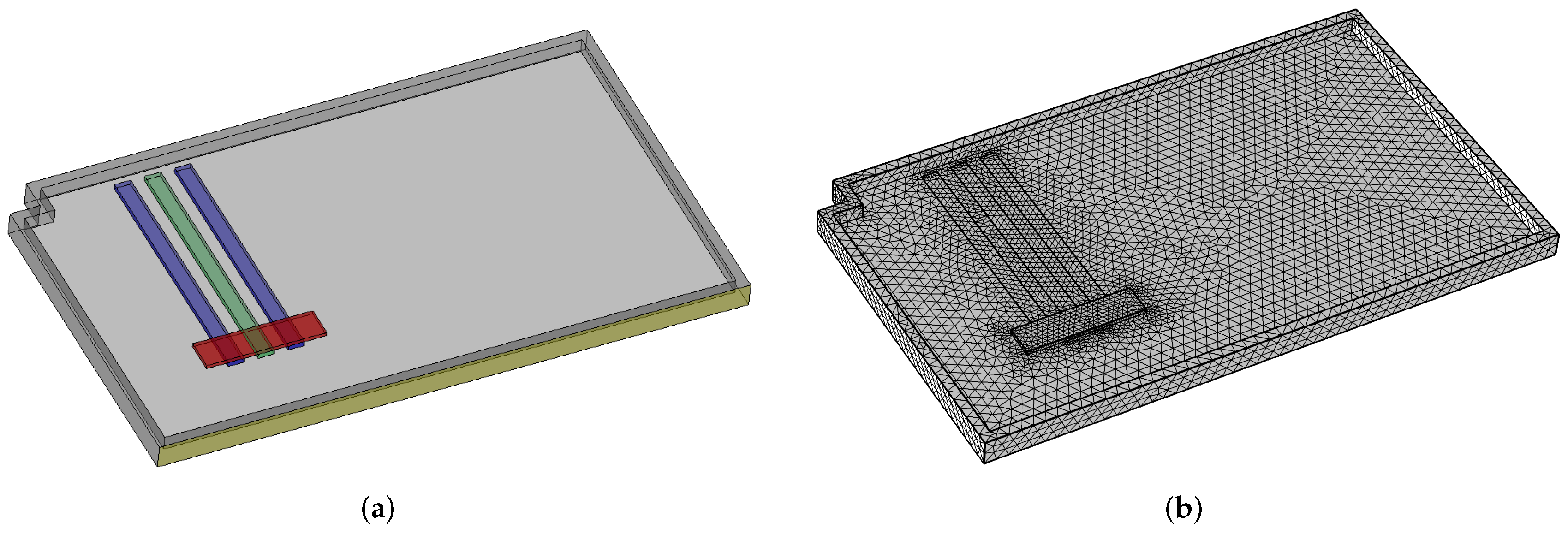
After defining the geometry, the domain is meshed with a standard tetrahedral mesh. Both the geometry and the mesh are shown in Figure 5.
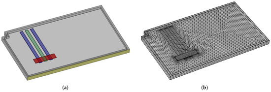
Figure 5.
Geometry (in green and blue—the three heat pipes, in red—the heat source) and mesh used for the preliminary CFD simulation (a) Geometry. (b) Mesh.
The heat pipes can exchange heat in different ways:
- Their sides and rear face can exchange by conduction with the chassis cover;
- Their front face can exchange by natural convection with the air in the room;
- Their front face can exchange also by radiation with the walls of the room.
Inside the chassis cover, heat is obviously transported by conduction. Then, all the external surfaces of the chassis cover can exchange heat by convection and radiation with the surroundings. Radiation is modeled with the simplifying assumption of “small body exchanging with a large cavity”. Emissivity of the surfaces is assumed as for the nontreated aluminum parts, while it is assumed as for the blackened faces. The convective coefficient between the chassis cover and the surrounding air is roughly assumed as uniform on all faces, and estimated by correlations for natural convection over a vertical flat plate (resulting in a value of ).
The input thermal power given by the resistor is modeled as a periodic rectangular wave with duty cycle ( pulse width, total cycle duration) and maximum power . The results of the simulation provide the temperature evolution of the whole chassis with the embedded heat pipes.
The temperature distribution on the chassis at four significant instants of time is shown in Figure 6 (at the end of the two phases of the first cycle) and Figure 7 (at the end of the two phases in a stabilized cycle). In particular, Figure 6a shows the temperature at the end of the first thermal charge phase, Figure 6b shows the temperature at the beginning of the second thermal charge phase, Figure 7a shows the temperature at the end of the last thermal charge phase, and Figure 7b shows the temperature at the end of the last thermal discharge phase.
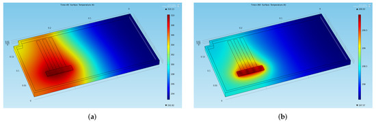
Figure 6.
Temperature distribution obtained through the preliminary CFD simulation at two significant instants of time in the first cycles (a) End of the first thermal charge phase: . (b) Beginning of the second thermal charge phase: .
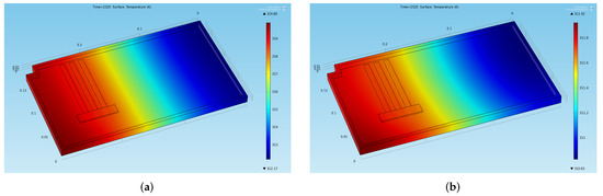
Figure 7.
Temperature distribution obtained through the preliminary CFD simulation at two significant instants of time in the stabilized cycles (a) End of the last thermal charge phase: . (b) End of the last thermal discharge phase: .
The temperature evolution of the central heat pipe is extracted and given as an input to a MATLAB code. In this code, the heat pipe is modeled by using a single-node lumped parameter approach, with the following assumptions:
- The input thermal power, , is constant and equal for all the thermal charge phases, and it is null for all the thermal discharge phases;
- The value of the resistance is constant during the phases of charge and discharge of the same cycle, while it changes between the cycles to take into account the equivalent convective coefficient variation with temperature.
Therefore, the two equations describing the temperature evolution of the heat pipe as a function of and are:
- For the thermal charge phases: ;
- For the thermal discharge phases: .
In the above, C is the equivalent heat capacity of the heat pipe.
In the previous equations, the equivalent heat capacity, the temperature, and the temperature derivative are assumed as known for each time step—they are obtained by sampling the temperature profile in time calculated by the transient CFD simulation in two points, corresponding to the positions of the thermocouples in the real experiment, and averaging them.
Consequently, for each thermal cycle, the MATLAB code computes from the second equation and then from the first equation, thus returning the two needed pieces of input data.
4. Results
In this section, the results obtained using the described model will be presented. The section is divided in two parts: the first one describes the comparison between numerical and experimental data for the case study, while the second one focuses on the analysis of the model accuracy when using the ideal and real gas assumptions, for a representative simulation with constant input power, using different fluids.
4.1. Model Validation
By using the input parameters described in Section 3.3, the simulation is run. As previously mentioned, the total time for the seven cycles is , which corresponds to . Since the ODEs of the model are approximated through the forward finite differences method, which is an explicit method, a small time step is needed to keep the simulations stable. After some preliminary tests, a fixed time step equal to 5 μs was selected.
In the experiment, two thermocouples were placed on the two opposite extremities of the central heat pipe. In particular, the one closer to the resistor acquires a temperature that will be indicated with the symbol in the following, while the other one acquires a temperature that will be indicated with the symbol in the following.
Since the thermocouples are placed on the external wall of the heat pipe, at the two opposite extremities, it is reasonable to compare with the evaporator wall temperature, , and with the condenser wall temperature, . It is worth noting that the results are partially biased by the fact that the real evaporator wall temperature is the one of the heat pipe face below the resistor, so it is reasonably higher than . Moreover, the condenser wall temperature computed by the model is the temperature at the center of the condenser wall. Thus, since more than the of the heat pipe length is taken up by the condenser, its center is not close to its end. Consequently, in practice, it must be taken into account that cannot be exactly equal to .
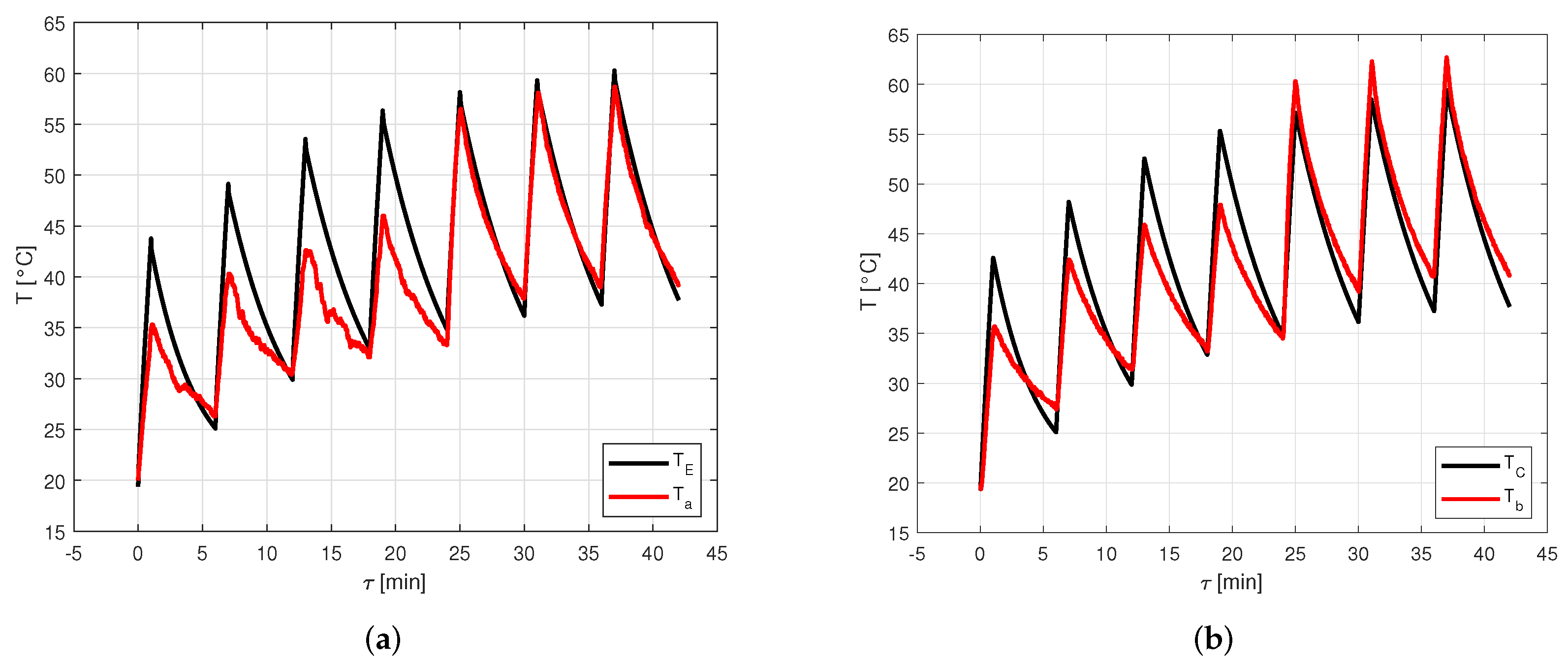
Figure 8 shows the comparison between numerical data computed through the model and experimental data acquired by the thermocouples for the seven thermal cycles. In particular, Figure 8a shows the comparison between and , while Figure 8b shows the comparison between and .
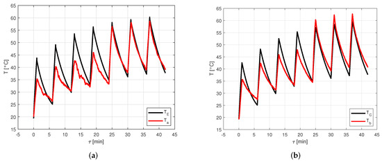
Figure 8.
Comparison between numerical data computed through the model and experimental data acquired by the thermocouples for the seven thermal cycles. (a) Comparison between and . (b) Comparison between and .
From Figure 8, it is possible to see that the model provides results very close to the experimental ones in the last three cycles, namely, the stabilized ones. In fact, in these cycles, the error on the peaks of the evaporator temperature goes from to , with an average value of , while the error on the peaks of the condenser temperature covers the range between and , with an average value of . Conversely, in the first four cycles, the maximum temperature of each cycle estimated by the model is much higher than the measured one, even if the minimum temperature for each cycle is very close to the experimental one. In these cycles, the error on the peaks of the evaporator temperature goes from to , with an average value of , while the error on the peaks of the condenser temperature covers the range between and , with an average value of .
The temperature evolution computed by the model is more regular than the measured one. This can be explained by the fact that when the heat pipe operation starts, the activation process takes a certain time, which varies depending on the considered heat pipe. In its present version, the activation process in the model is idealized, no activation resistances are considered.
In the experimental test analyzed, the heat pipe activation process reasonably takes a significant fraction of the total time for the first thermal charge phases, so, at the end, the heat pipe has not reached a temperature as high as it would have with a lower or null activation time. However, after four cycles, the temperature reached is high enough to stabilize the following cycles, so the model becomes much more reliable.
From Figure 8b, it is possible to notice that in the last three cycles, the measured temperature is higher than the one predicted by the model. This discrepancy is probably due to how the input data are extracted. In fact, after a preliminary CFD simulation, the boundary conditions are obtained by approximating the heat pipe through a single-node lumped parameter approach. When using this method, it is assumed that each region of the heat pipe exchanges the same amount of heat. However, in the real case, it is reasonable to assume that the heat exchanged by the front face of the condenser, by natural convection and radiation, is lower than the heat exchanged by the other faces of the condenser, by conduction with the chassis cover. Therefore, the temperature of the condenser external wall, which can be computed as an average of the temperatures of the whole external wall of the condenser, may be lower than .
Therefore, it is possible to state that, in view of the results of the comparison between the numerical data computed through the model and experimental data acquired by the thermocouples for the seven thermal cycles, the validation of the model can be considered satisfactory, despite some predictable limitations.
4.2. Comparison between Ideal and Real Gas
In this subsection, four fictitious cases with constant evaporator heat power are considered. The heat pipe considered is the one used for the case study in terms of shape and dimensions, but the analysis is performed by considering four different solid–fluid couples, namely, copper–water, aluminum–ammonia, aluminum–acetone, and copper–HFC134a refrigerant. For each case, the vapor temperatures and pressures obtained by using the model proposed in this work are compared with the ones obtained by modeling the vapor as an ideal gas, as in the work of Ferrandi et al. [8].
In order to perform such analysis, it is assumed that the considered heat pipe is subject to a constant heat power input equal to , and the resistance is modeled as an equivalent convective resistance. The initial temperature and the external temperature are both set to be equal to 25 °C. Furthermore, it is assumed, without loss of generality, that the heat pipe is oriented horizontally.
4.2.1. Copper-Water
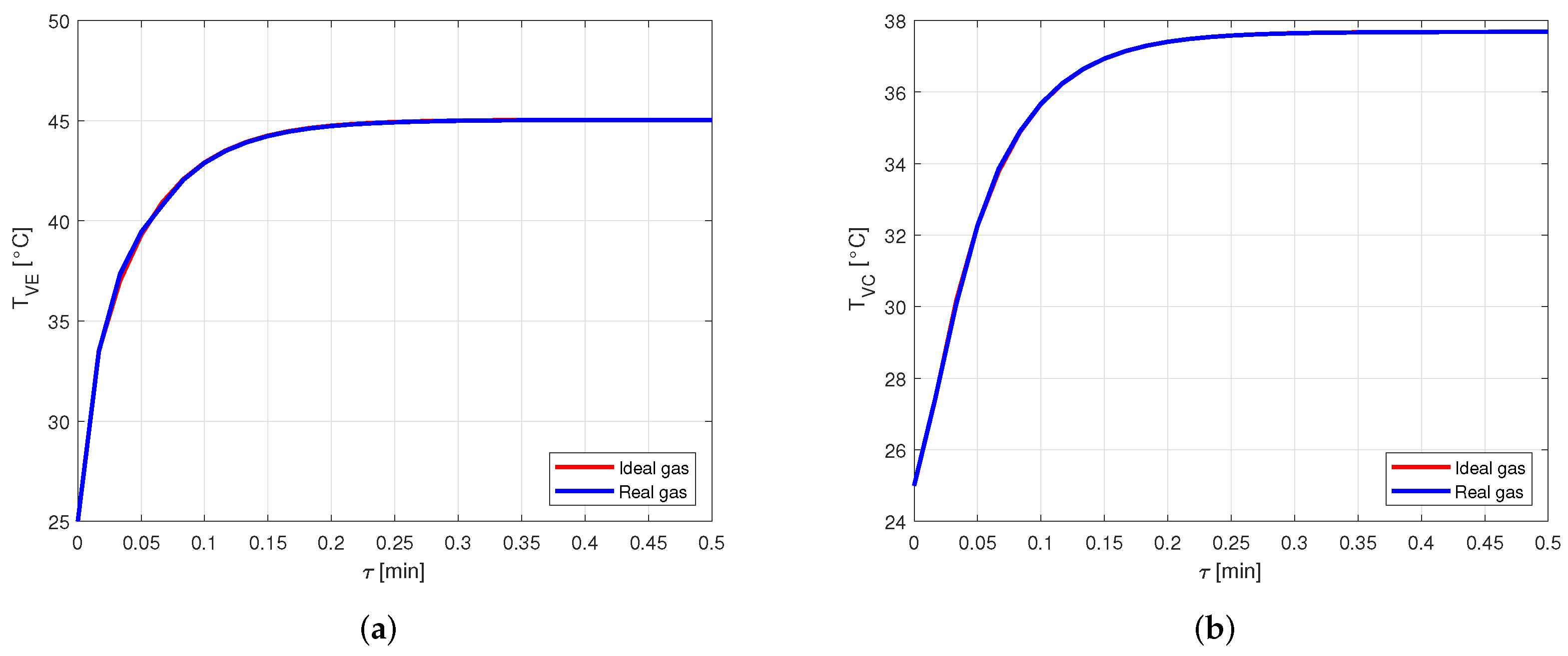
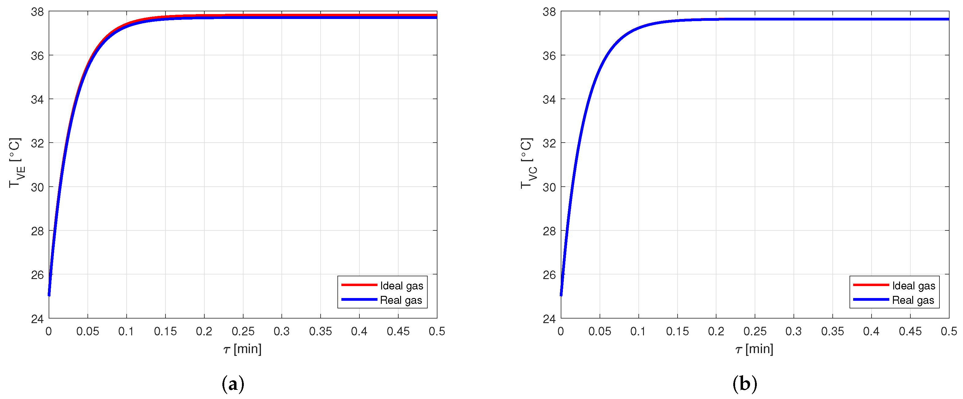
Figure 9 shows the comparison between the vapor temperatures in case of using ideal or real gas equations for the vapor modeling, in a heat pipe made of copper and filled with water as working fluid. In particular, Figure 9a shows the comparison between the vapor temperatures in the evaporator, , while Figure 9b shows the comparison between the vapor temperatures in the condenser, .
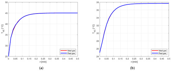
Figure 9.
Comparison between the vapor temperatures obtained by modeling the vapor as ideal or real gas, in a copper-water heat pipe (a) Comparison of the vapor temperatures at the evaporator. (b) Comparison of the vapor temperatures at the condenser.
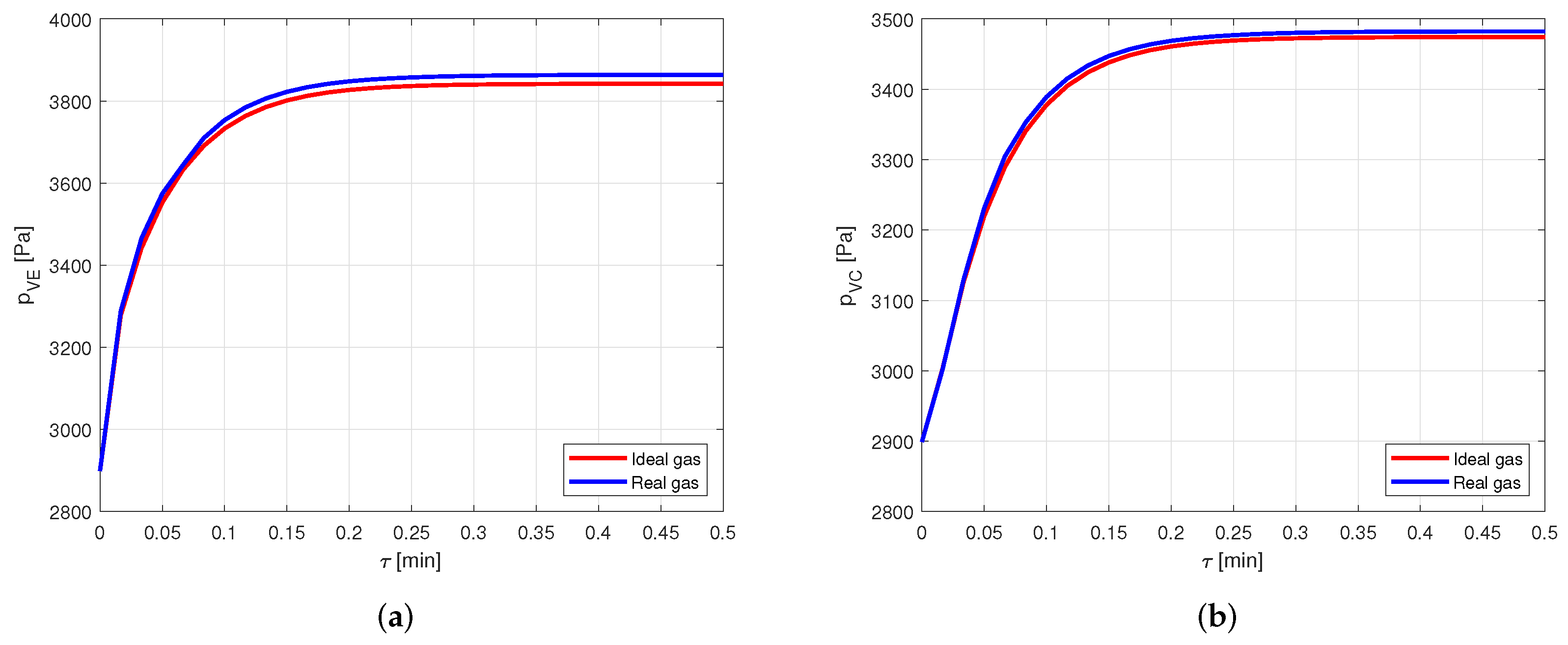
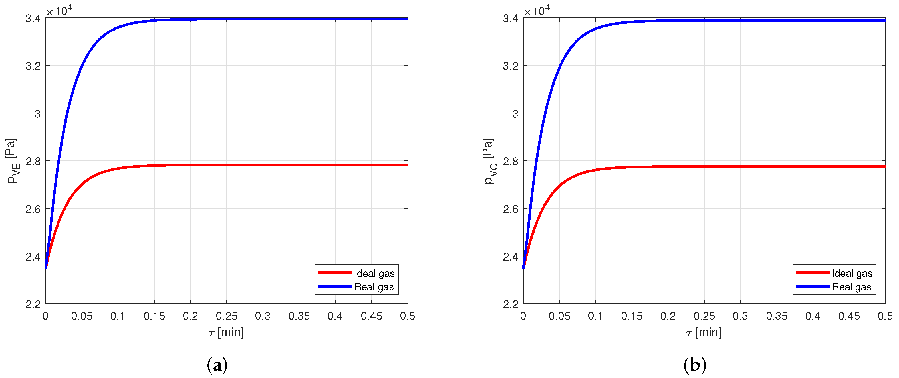
It is evident how the vapor temperatures in the two cases are practically equal. Looking at the vapor pressures in the evaporator, in Figure 10a, and in the condenser, in Figure 10b, it is possible to notice a small difference in the results when the steady state is reached.
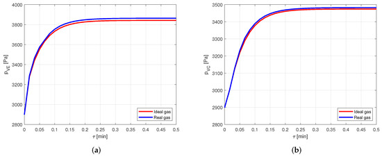
Figure 10.
Comparison between the vapor pressures obtained by modeling the vapor as ideal or real gas, in a copper-water heat pipe. (a) Comparison of the vapor pressures at the evaporator. (b) Comparison of the vapor pressures at the condenser.
Nevertheless, this difference leads to an error lower than in the pressure estimation. Therefore, for the given conditions, modeling the vapor as a real gas is not necessary when the considered fluid is water. This is reasonable, as the compressibility factor of water in the considered case is very close to the one in [22], confirming the fact that water vapor behaves almost as an ideal gas.
4.2.2. Aluminum–Ammonia
As a second case, the same simulation was repeated using a heat pipe made of aluminum and filled with ammonia as working fluid.
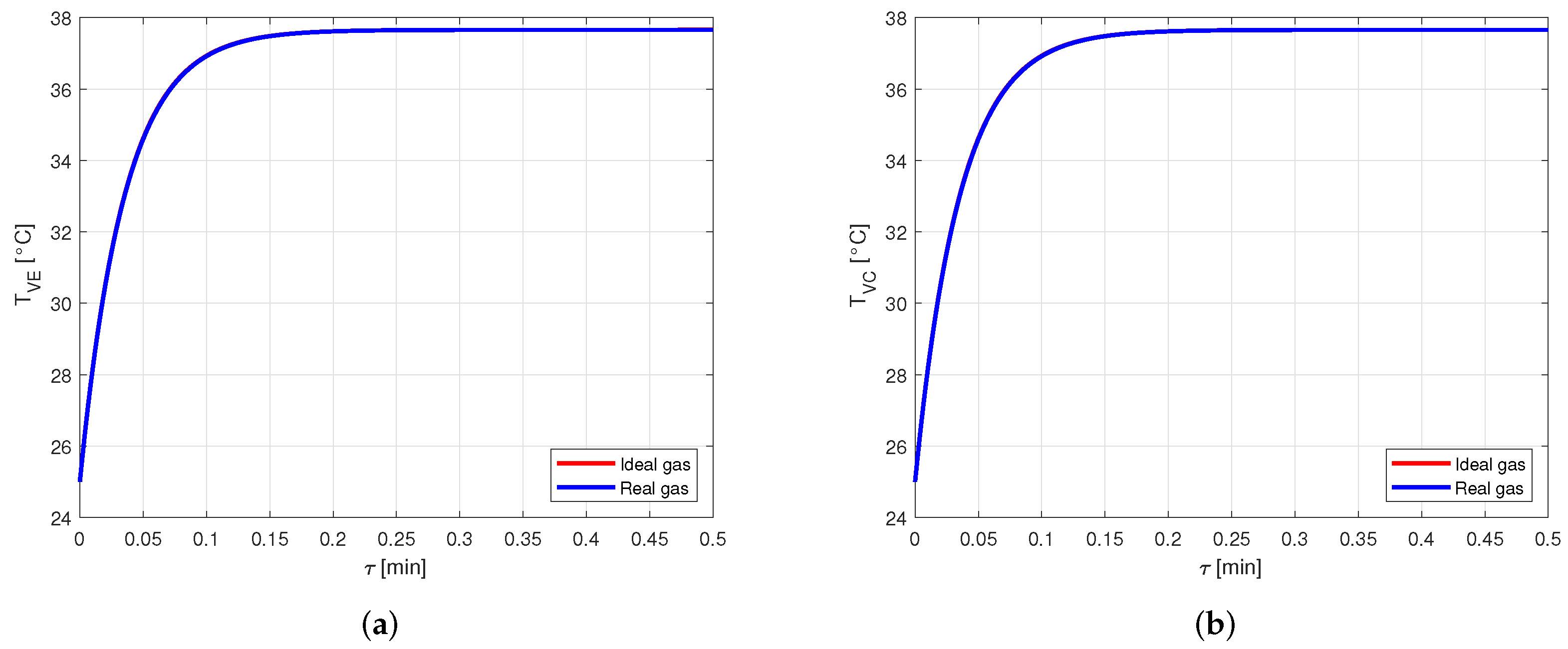
The difference between the vapor temperatures computed by approximating the vapor as ideal or real gas are shown in Figure 11.
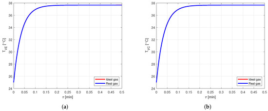
Figure 11.
Comparison between the vapor temperatures obtained by modeling the vapor as ideal or real gas, in an aluminum-ammonia heat pipe. (a) Comparison of the vapor temperatures at the evaporator. (b) Comparison of the vapor temperatures at the condenser.
Again, it is possible to notice that the temperature profiles are similar to the point that it is hard to distinguish the respective curves.
The comparison between the vapor pressure curves in case of ideal and real gas shows a difference of about , as can be seen in Figure 12. This difference can be relevant in some applications, but, in general, such an error will be much lower than those caused by the use of the lumped parameter approach, so for this case also it can be concluded that there is no relevant difference in modeling the vapor as ideal or real gas.
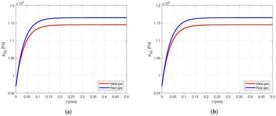
Figure 12.
Comparison between the vapor pressures obtained by modeling the vapor as ideal or real gas, in an aluminum-ammonia heat pipe. (a) Comparison of the vapor pressures at the evaporator. (b) Comparison of the vapor pressures at the condenser.
4.2.3. Aluminum–Acetone
At this stage, the same case as before is analyzed, but using a heat pipe made of aluminum and filled with acetone as working fluid.
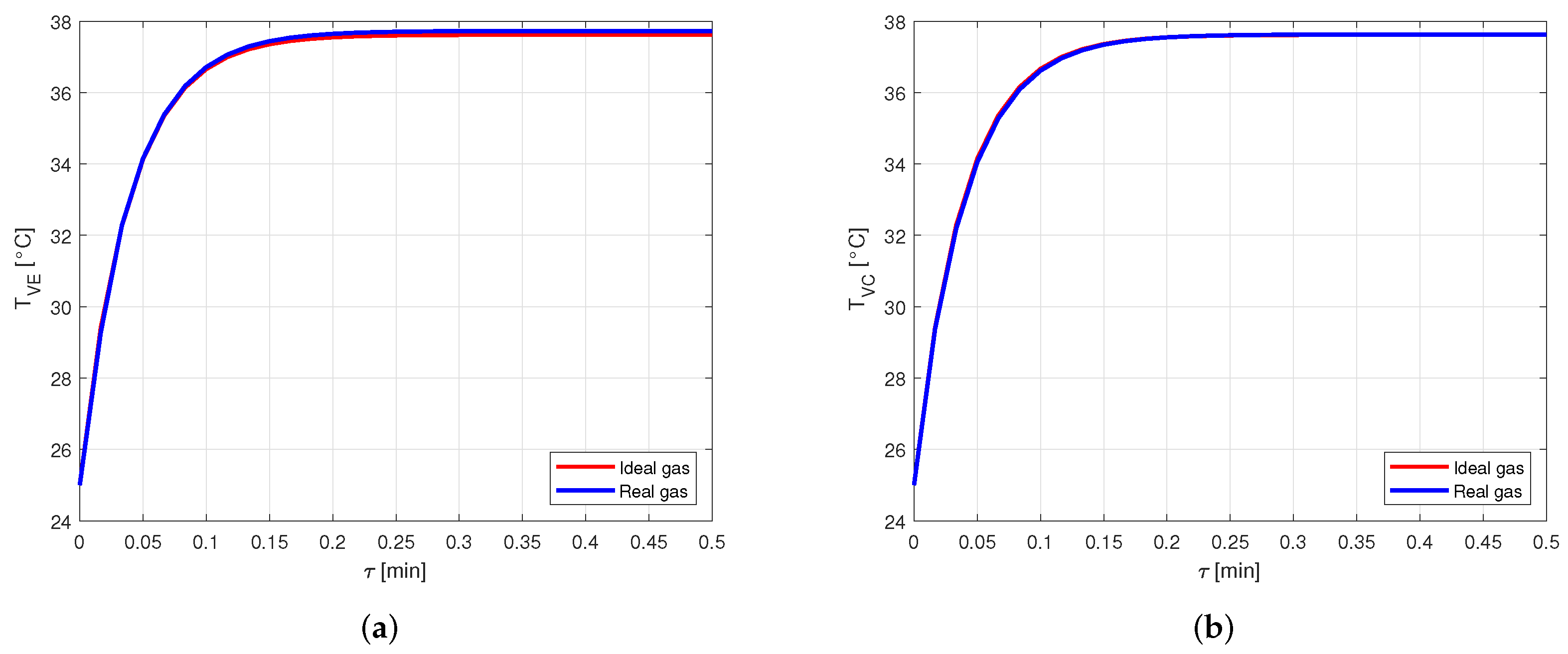
The comparison between the vapor temperatures obtained in case of modeling the vapor as ideal or real gas is shown in Figure 13 and, as in the previous cases, the difference between the curves is negligible.
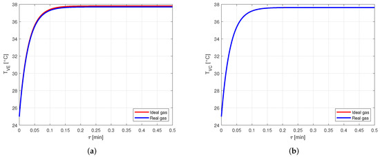
Figure 13.
Comparison between the vapor temperatures obtained by modeling the vapor as ideal or real gas, in an aluminum-acetone heat pipe. (a) Comparison of the vapor temperatures at the evaporator. (b) Comparison of the vapor temperatures at the condenser.
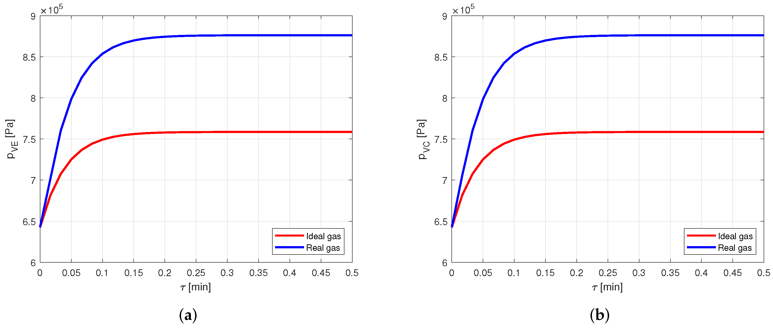
However, comparing the vapor pressures in the two cases (Figure 14), it is possible to notice that the error in modeling the vapor as an ideal gas rather than a real gas is close to , and this is certainly not negligible.
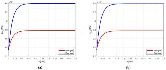
Figure 14.
Comparison between the vapor pressures obtained by modeling the vapor as ideal or real gas, in an aluminum-acetone heat pipe. (a) Comparison of the vapor pressures at the evaporator. (b) Comparison of the vapor pressures at the condenser.
Therefore, when acetone is used as working fluid, it is necessary to model the vapor by using the real gas equations.
4.2.4. Copper–HFC134a Refrigerant
Finally, again the same case is analyzed, but using a heat pipe made of copper and filled with HFC134a as working fluid.
The results are the same of the acetone–aluminum case: the temperature profiles (Figure 15) show a practically null difference, while the pressure profiles (Figure 16) evidence a deviation of more than .
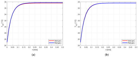
Figure 15.
Comparison between the vapor temperatures obtained by modeling the vapor as ideal or real gas, in a copper-HFC134a heat pipe. (a) Comparison of the vapor temperatures at the evaporator. (b) Comparison of the vapor temperatures at the condenser.
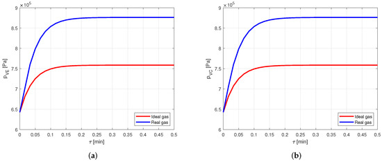
Figure 16.
Comparison between the vapor pressures obtained by modeling the vapor as ideal or real gas, in a copper-HFC134a heat pipe. (a) Comparison of the vapor pressures at the evaporator. (b) Comparison of the vapor pressures at the condenser.
Therefore, also when using HFC134a as working fluid of the heat pipe, modeling the vapor as a real gas offers a significant increase in the accuracy.
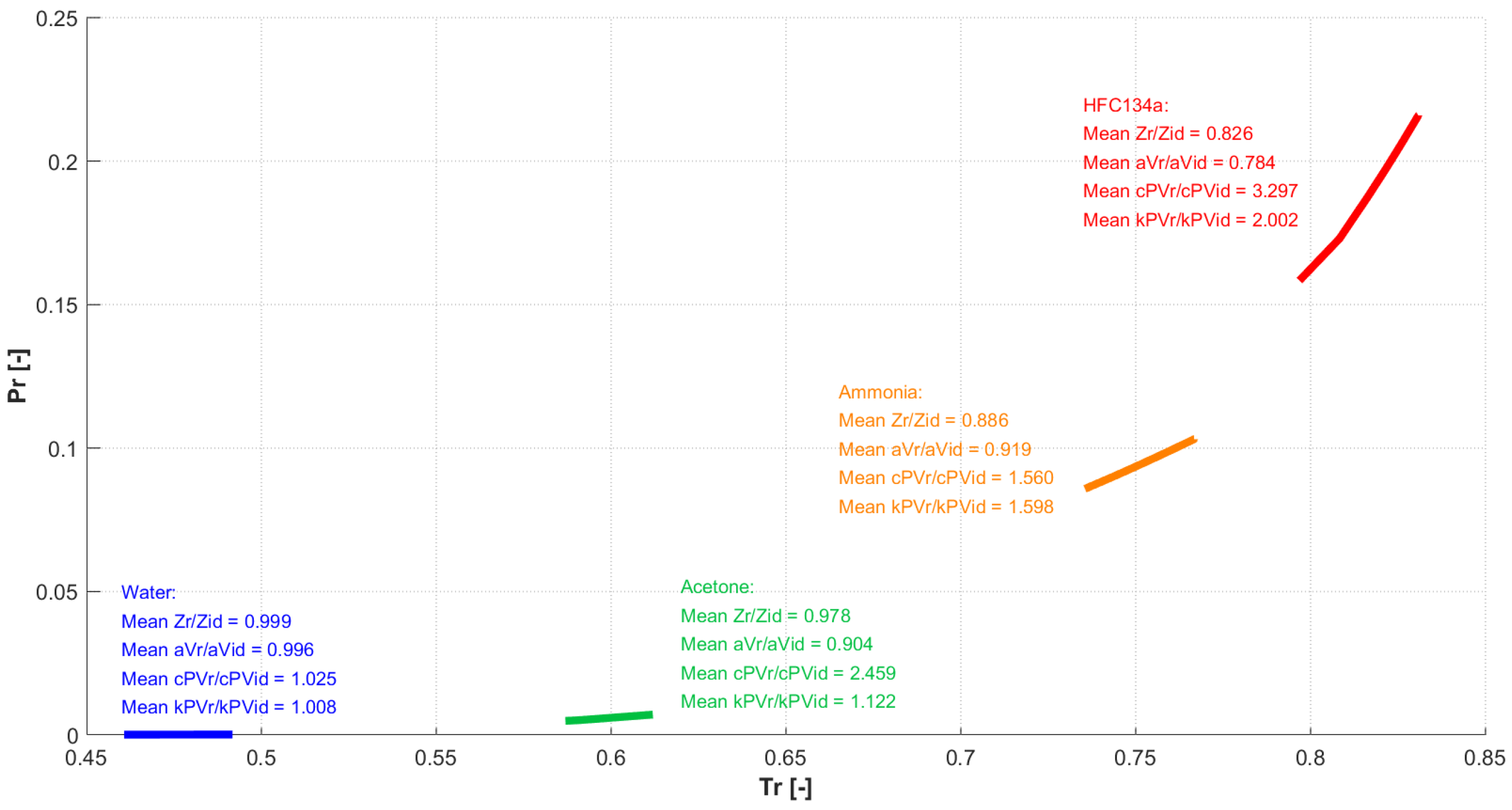
In summary, the results confirmed that when the working fluid and the operating conditions are such that the intermolecular forces play a significant role, real gas equations and properties should be used. The amount of deviation from the ideal gas behavior at a certain temperature and pressure depends on the specific substance. To better evidence this aspect, Figure 17 shows the paths followed by the four fluids (water, ammonia, acetone, HFC134a) in the evaporator, during the transition from start-up to steady operation, in a chart (using reduced thermodynamic properties, and ).
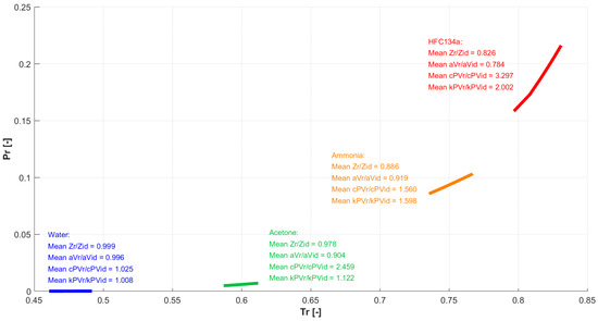
Figure 17.
Paths followed by the four fluids in the evaporator during the thermal transient.
As it can be seen, the fluids work in different regions. The average ratios between real gas and ideal gas values for compressibility, speed of sound, isobaric specific heat, and isobaric expansion coefficient are also reported. The latter evidence how for some fluids the values are all close to unity, and this is reflected in a negligible difference between real and ideal gas predictions, while for others the difference is large, resulting in the need for real gas modeling.
5. Conclusions
In this study, a multinode lumped parameter model for steady and transient analysis of heat pipes was developed, starting from other models already existing in literature, but including the effects of gravity (orientation angle) and modeling the vapor as a real gas.
The model was validated by using an experimental case study, in which three parallel heat pipes were embedded in a chassis cover and heated by a resistor, during seven cycles of of thermal charge and of thermal discharge.
The evaporator and condenser wall temperatures of the heat pipe in the middle, measured by two thermocouples, were compared to the ones obtained through the model. The results showed good agreement in predicting data in the stabilized thermal cycles, while the model provides temperatures much higher than the measured ones in the first cycles. This is probably due to the heat pipe activation process, the method through which the boundary conditions were calculated, and also to the position of the thermocouples which acquired the experimental results.
Additionally, it is analyzed whether, for some working fluids, it is important to model the vapor as a real gas, rather than as an ideal gas. This analysis showed that the vapor temperatures obtained by modeling the vapor as an ideal or real gas are almost the same, for all the considered cases. However, the vapor pressures can be significantly different.
In particular, when using water or ammonia as working fluids, the difference between the vapor pressures is negligible, while when using acetone or HFC134a as working fluids, modeling the vapor as an ideal gas rather than a real gas leads to an error in the vapor pressure prediction larger than .
Therefore, it can be concluded that when the operating conditions are such that the intermolecular forces play a significant role, it becomes important to model the working fluid as a real gas, both in terms of relations and of values of the thermophysical properties included in the model. Otherwise, the latter may be significantly under- or overestimated, resulting in a bad prediction, particularly of the vapor pressures.
Author Contributions
Conceptualization, all authors; methodology, R.C. and M.G.; resources, L.G., R.I. and M.M.; software, R.C.; investigation, R.C. and M.G.; formal analysis, R.C. and M.G.; validation, all authors; writing—original draft preparation, R.C.; writing—review and editing, all authors; Visualization, R.C. All authors have read and agreed to the published version of the manuscript.
Funding
This research received no external funding.
Data Availability Statement
The results of the numerical simulations are available from the authors upon reasonable request.
Conflicts of Interest
The authors declare no conflict of interest.
Nomenclature
The following symbols and subscripts are used in this manuscript:
| Symbols: | |
| A | Area [m2] |
| diagonal matrix of the coefficients multiplying the | |
| derivatives of the solid network unknowns [WsK−1] | |
| a | Speed of sound [ms−1] |
| symmetric matrix of the coefficients multiplying the | |
| solid network unknowns [KW−1] | |
| C | Capacitance of a thermal equivalent condenser [WsK−1] |
| vector of the constant terms | |
| c | Specific heat [J kg−1 K−1] |
| Specific heat at constant pressure [J kg−1 K−1] | |
| Hydraulic diameter | |
| f | Body force per unit volume [Nm−3] |
| g | Gravity acceleration [ms−2] |
| h | Convective coefficient [Wm−2 K−1] |
| Latent heat of vaporization [J kg−1] | |
| K | Wick permeability [m2] |
| Isobaric expansion coefficient [K−1] | |
| identity matrix | |
| L | Length |
| l | Variable of integration |
| Mass flow rate [kg s−1] | |
| N | Total number of vapor mass flow rates crossing the vapor |
| tank boundaries | |
| n | Current time step |
| P | Perimeter |
| p | Pressure |
| Heat power | |
| R | Resistance of a thermal equivalent resistor [WK−1] |
| r | Radius |
| Reynolds number | |
| s | Specific entropy [J kg−1 K−1] |
| T | Temperature |
| t | Thickness |
| u | Vapor velocity [ms−1] |
| V | Volume [m3] |
| w | Weight/Width |
| x | One-dimensional coordinate |
| vector of the temperatures of the solid network | |
| Heat pipe orientation angle | |
| Wick porosity | |
| Contact angle | |
| Thermal conductivity [Wm−1 K−1] | |
| Dynamic viscosity | |
| Density [kgm−3] | |
| Surface tension [Nm−1] | |
| Time | |
| Subscripts: | |
| 0 | Initial |
| 1 | Node 1 |
| 2 | Node 2 |
| A | Adiabatic zone/Axial |
| C | Condenser zone/Condensing/Circular |
| c | Capillary |
| E | Evaporator zone/Evaporating |
| Effective | |
| External wall | |
| Equivalent | |
| External wick | |
| F | Referred to a thermal exchange by convection |
| i | Summation index |
| Entering the system | |
| Internal wall | |
| Internal wick | |
| L | Liquid/Linear |
| M | Mixed |
| m | Mean/Molar |
| n | Referred to a generic node |
| Exiting the system | |
| P | Solid wall |
| p | Pore/Solid wall |
| R | Radial |
| r | Reduced |
| Saturation | |
| Total | |
| V | Vapor zone/Vapor |
| W | Wick |
| w | Wick |
| x | One dimensional coordinate |
Appendix A. Details about the Numerical Implementation
In order to solve the twenty equations of System (33), the following numerical method has been used.
The first six equations to be solved in the iterative cycle covering all the time steps are the ones describing the solid network. For each time step, the vapor temperatures , , and (which is a linear combination of and ) are evaluated at the previous time step, so that the six equations for the solid network have six unknowns (, , , , , ), and can be solved all together before the others. In particular, they are rewritten as:
Defining a vector , which contains the unknowns:
it is possible to write System (A1) in matrix form, as:
where:
- is the diagonal matrix which contains the coefficients that multiplies the derivatives of the unknowns, namely the capacitances;
- is the symmetric matrix which contains the coefficients that multiplies the unknowns, namely the inverse of the solid resistances;
- is the vector of the constant terms, namely the one representing the heat transfer rates entering and exiting the solid network.
At this point, using the forward finite differences approach, Equation (A3) can be rewritten in discrete form as:
where: the superscripts and indicate the current and the following time steps, respectively; and indicates the time step.
Since matrix is diagonal, its inversion is straightforward. In fact, is the diagonal matrix whose coefficients are the inverse of the ones of . This property makes the computational cost of the inversion of significantly lower.
Therefore, vector at time can be computed starting from the same vector at time , by inverting Equation (A4) as:
where: is the identity matrix.
After that, the fourteenth, eighth, ninth, tenth, and eleventh equations of System (33) are rewritten as:
where the definitions of and , merged with the definitions of and , are exploited.
At this point, System (A6) can be rewritten in discrete form by using the forward finite differences, and solved similarly to the one for the solid network, as:
Therefore, for each time step, the eleven equations of Systems (A5) and (A7) are solved, in order to find eleven variables: , , , , , , , , , , . The remaining nine variables are not computed in the iterative cycle, but for all the time steps sequentially after it, as:
After solving System (A8), all the variables of the problem have been computed.
References
- Shukla, K. Heat pipe for aerospace applications—An overview. J. Electron. Cool. Therm. Control 2015, 5, 1. [Google Scholar] [CrossRef] [Green Version]
- Jouhara, H.; Chauhan, A.; Nannou, T.; Almahmoud, S.; Delpech, B.; Wrobel, L.C. Heat pipe based systems-Advances and applications. Energy 2017, 128, 729–754. [Google Scholar] [CrossRef]
- Elnaggar, M.H.; Edwan, E. Heat pipes for computer cooling applications. In Electronics Cooling; InTech: Rijeka, Croatia, 2016; p. 51. [Google Scholar]
- Velardo, J.; Singh, R.; Date, A.; Date, A. An investigation into the effective thermal conductivity of vapour chamber heat spreaders. Energy Procedia 2017, 110, 256–261. [Google Scholar] [CrossRef]
- Cullimore, B.; Baumann, J. Steady State and Transient Loop Heat Pipe Modeling. In Proceedings of the International Conference On Environmental Systems, Toulouse, France, 10 July 2000. [Google Scholar]
- Suman, B.; De, S.; DasGupta, S. Transient modeling of micro-grooved heat pipe. Int. J. Heat Mass Tran. 2005, 48, 1633–1646. [Google Scholar] [CrossRef]
- Ferrandi, C.; Marengo, M.; Zinna, S. Influence of Tube Size on Thermal Behaviour of Sintered Heat Pipe. In Proceedings of the 2nd European Conference on Microfluidics, Toulouse, France, 8–10 December 2010. [Google Scholar]
- Ferrandi, C.; Iorizzo, F.; Mameli, M.; Zinna, S.; Marengo, M. Lumped parameter model of sintered heat pipe: Transient numerical analysis and validation. Appl. Therm. Eng. 2013, 50, 1280–1290. [Google Scholar] [CrossRef]
- Bernagozzi, M.; Charmer, S.; Georgoulas, A.; Malavasi, I.; Michè, N.; Marengo, M. Lumped parameter network simulation of a Loop Heat Pipe for energy management systems in full electric vehicles. Appl. Therm. Eng. 2018, 141, 617–629. [Google Scholar] [CrossRef]
- Wang, X.; Li, B.; Yan, Y.; Gao, N.; Chen, G. Predicting of thermal resistances of closed vertical meandering pulsating heat pipe using artificial neural network model. Appl. Therm. Eng. 2019, 149, 1134–1141. [Google Scholar] [CrossRef]
- Guichet, V.; Khordehgah, N.; Jouhara, H. Experimental investigation and analytical prediction of a multi-channel flat heat pipe thermal performance. Int. J. Thermofluids 2020, 5, 100038. [Google Scholar] [CrossRef]
- Zimmermann, S.; Dreiling, R.; Nguyen-Xuan, T.; Pfitzner, M. An advanced conduction based heat pipe model accounting for vapor pressure drop. Int. J. Heat Mass Tran. 2021, 175, 121014. [Google Scholar] [CrossRef]
- Guilizzoni, M. La Fisica Tecnica e il Rasoio di Ockham; Maggioli Editore: Santarcangelo di Romagna (RM), Italy, 2017. [Google Scholar]
- Payne, L.; Rodrigues, J.; Straughan, B. Effect of anisotropic permeability on Darcy’s law. Math. Method Appl. Sci. 2001, 24, 427–438. [Google Scholar] [CrossRef]
- Byon, C.; Kim, S.J. Capillary performance of bi-porous sintered metal wicks. Int. J. Heat Mass Tran. 2012, 55, 4096–4103. [Google Scholar] [CrossRef]
- Pal, R. Teach second law of thermodynamics via analysis of flow through packed beds and consolidated porous media. Fluids 2019, 4, 116. [Google Scholar] [CrossRef] [Green Version]
- de Laplace, P.S. Traité De Mécanique Céleste: Supplément au Dixième Livre du Traité de Méchanique Céleste sur l’action Capillaire; Duprat: Paris, France, 1808; Volume 6. [Google Scholar]
- National Institute of Standards and Technology. 2021. Available online: https://www.nist.gov (accessed on 13 December 2021).
- Incropera, F.P.; Lavine, A.S.; Bergman, T.L.; DeWitt, D.P. Fundamentals of Heat and Mass Transfer; Wiley: Hoboken, NJ, USA, 2007. [Google Scholar]
- Mitropoulos, A.C. The Kelvin equation. J. Colloid Interface Sci. 2008, 317, 643–648. [Google Scholar] [CrossRef] [PubMed]
- Comsol—Software for Multiphysics Simulation. 2021. Available online: https://www.comsol.com/ (accessed on 26 December 2021).
- Nezbeda, I. Simulations of vapor–liquid equilibria: Routine versus thoroughness. J. Chem. Eng. Data 2016, 61, 3964–3969. [Google Scholar] [CrossRef]


Publisher’s Note: MDPI stays neutral with regard to jurisdictional claims in published maps and institutional affiliations. |
© 2022 by the authors. Licensee MDPI, Basel, Switzerland. This article is an open access article distributed under the terms and conditions of the Creative Commons Attribution (CC BY) license (https://creativecommons.org/licenses/by/4.0/).