Large-Eddy Simulation of a Classical Hydraulic Jump: Influence of Modelling Parameters on the Predictive Accuracy

Abstract

Results from large-eddy simulations of a classical hydraulic jump at inlet Froude number two are reported. The computations were performed using the general-purpose finite-volume-based code OpenFOAM^®, and the primary goal was to evaluate the influence of the modelling parameters on the predictive accuracy, as well as establish the associated best-practice guidelines. A benchmark simulation was conducted on a grid with a 1 mm-cell-edge length to validate the solver and provide a reference solution for the parameter influence study. The remaining simulations covered different selections of the modelling parameters: geometric vs. algebraic interface capturing, three mesh resolution levels, and four choices of the convective flux interpolation scheme. Geometric interface capturing led to better accuracy, but deteriorated the numerical stability and increased the simulation times. Interestingly, numerical dissipation was shown to systematically improve the results, both in terms of accuracy and stability. Strong sensitivity to the grid resolution was observed directly downstream of the toe of the jump.

1. Introduction

A hydraulic jump is an abrupt change in the water depth accompanying the transition of the flow from supercritical to subcritical. This transition causes energy dissipation, which defines the application of hydraulic jumps in engineering. In fact, according to [1], hydraulic jumps are the most commonly used energy dissipators in hydraulic structures. However, the hydraulic jump is also a natural environmental phenomenon, occurring in rivers and bays. This motivates the significant attention this class of flows has received from the scientific community. Hydraulic jumps have been the subject of a multitude of studies, both experimental and numerical; recent reviews can be found in [2,3]. Most works focuses on the so-called “classical” hydraulic jump (CHJ), which occurs in a smooth horizontal rectangular channel.

An illustration of the air-water interface in a CHJ is shown in Figure 1. The topology of the interface is complex and rapidly evolving, which can be fully appreciated by looking at the animations found in the archive published alongside this article (see the Data Availability Statement). The interface dynamics are driven by a recirculating motion—the so-called roller—which leads to overturning waves occurring across the jump.

Consequently, a significant amount of air is entrained. A detailed discussion of the entrainment mechanism can be found in [4]. The flow in the jump is also highly turbulent, with a turbulent shear layer forming below the roller and interacting with it.

The main physical parameter of the CHJ is the inlet Froude number, ${\mathrm{Fr}}_1$, computed based on the water inlet velocity, $U_1$, and its depth, $d_1$. Several classifications of the jump’s behaviour based on ${\mathrm{Fr}}_1$ can be found in the literature; see [2] and the references therein. The most stable CHJs occur when ${\mathrm{Fr}}_1\in [4,9]$. The rate of air entrainment also depends on the Froude number, and at higher ${\mathrm{Fr}}_1$, the level of aeration increases. Here, we considered a jump at ${\mathrm{Fr}}_1=2$, which corresponds to the “weak jump” [5] regime. It is characterised by a relatively thick jet at low velocity entering the jump and a relative energy loss of about 7% [6].

In spite of the flow’s complexity, given the parameters of the inflow, some of its properties can be easily derived analytically based on control volume analysis; see e.g., [7] (p. 250). This includes the water depth after the jump, $d_2=0.5d_1\left({(1+8{\mathrm{Fr}}_1^2)}^{0.5}-1\right)$.

From a numerical perspective, the CHJ represents an extremely challenging test of predictive capabilities for multiphase modelling approaches. A suitable model should be able to capture fast and complex topology changes taking place across a wide range of spatial scales. Accurate turbulence modelling is also necessary and, in particular, the possibility to properly account for its interaction with the multiphase structures. On the other hand, the geometric simplicity of the case makes mesh generation easy, and the abundance of published experimental data makes validation easier. Furthermore, data from direct numerical simulation (DNS) [4] are also available.

A compilation of previous numerical studies of the CHJ, classified by turbulence modelling approach, and also ${\mathrm{Fr}}_1$, can be found in [3]. At the lowest level of fidelity, there are works where the jump is simulated using one-dimensional Boussinesq equations; see [8]. However, the majority of works are based on two-equation Reynolds-averaged Navier–Stokes (RANS) turbulence models and the volume of fluid (VoF) method for capturing the interface. Note that in RANS, it is assumed that there is a clear scale separation between the modelled turbulent motion and other types of unsteadiness. In the case of a CHJ, this is unlikely to take place due to the direct interaction between turbulence and multiphase structures, e.g., entrained bubbles. Generally, it is unclear whether the topological changes in the flow occur significantly slower than the integral time scales of turbulence. A possibility for resolving this inconsistency is keeping the resolution coarse enough for the interface to remain steady and introduce an explicit model for air entrainment, as performed in [9]. However, these theoretical difficulties do not imply that RANS cannot be used to obtain useful results. On the contrary, as summarised in [3], RANS is capable of predicting $d_2$, the mean location of the interface, and the length of the roller with a <5% relative error.

In order to obtain new physical insights and obtain an accurate picture of the turbulent motion inside the jump, scale-resolving turbulence modelling approaches can be used. Only a few studies have reported results from such simulations. The DNS by Mortazavi et al. [4] was already mentioned above and represents an important milestone. In [10,11], detached-eddy simulation (DES) was used. A detailed analysis of the flow was given; in particular, a quadrant decomposition of the turbulent shear stress was considered, as well as high-order statistical moments of the velocity field. A large-eddy simulation (LES) of a CHJ was conducted as part of the study by Gonzalez and Bombardelli, which also included RANS simulations [12]. Unfortunately, due to the reference being a short conference abstract, the results were only discussed superficially. In [13], the authors reported on an unsuccessful attempt to conduct an LES: the location of the jump could not be stabilised. Finally, in [9], which was already mentioned in the context of RANS, results from DES modelling were also discussed. However, the simulation in question was not a DES in the classical sense, i.e., not a fully resolved LES outside the RANS region. Instead, a rather coarse mesh was used, and an air entrainment model was employed. Nevertheless, this DES yielded more accurate results than the corresponding RANS.

With the increase of available computing power, it can be expected that LES and its hybrids will find wider adoption in hydraulic engineering in the near future. This transition is already well under way in, for example, the automotive and aerospace industries. From a practical perspective, an important step is to establish guidelines for the selection of the most important LES modelling parameters and understand the limitations in terms of accuracy that can be achieved at a given computational cost. Of immediate interest is to consider the particular case of solvers based on finite-volume discretisation, since these are currently the workhorse of industrial computational fluid dynamics. In this numerical framework, the two arguably most important LES input parameters are the density of the grid and the numerical scheme used for interpolating convective fluxes. Both control the capability of the LES to resolve turbulent structures, as well as the stability of the simulation. In the case of multiphase flow, the choice of the interface-capturing scheme is also important. The goal of this paper was to quantify the effects of these three parameters on the various quantities of interest. To that end, results from an LES campaign, consisting of 25 simulations of a CHJ at ${\mathrm{Fr}}_1=2$, are presented. This included a high-fidelity simulation with a similar resolution level as the DNS in [4]. In total, the campaign covered four different mesh resolution levels and two VoF approaches: algebraic and geometric. The diffusivity of the convective flux interpolation scheme was also controlled, and four diffusivity levels were considered. All the simulation results, including ready-to-run simulation cases, are made available as a supplementary dataset (see the Data Availability Statement).

The remainder of the article is structured as follows. Section 2 presents the computational fluid dynamics methods used in the paper. The setup of the CHJ simulations is presented in Section 3. The results of the simulation campaign are shown and analysed in Section 4. Finally, concluding remarks are given in Section 5.

2. Computational Fluid Dynamics Methods

2.1. Governing Equations

The volume of fluid (VoF) method [14] was used to simulate the flow. Accordingly, a single set of conservation equations was solved for both fluids, and the phase was distinguished based on the values of the volume fraction of the liquid, $\alpha$. The momentum and continuity equations read as follows,

$$\begin{array}{cc}\hfill \frac{\partial \rho u_i}{\partial t}+\frac{\partial }{\partial x_j}\left(\rho u_i{u}_j\right)& =-\frac{\partial p_{\rho gh}}{\partial x_i}-g_i{x}_i\frac{\partial \rho }{\partial x_i}+\frac{\partial }{\partial x_j}\left(\mu \left(\frac{\partial u_i}{\partial x_j}+\frac{\partial u_j}{\partial x_i}\right)\right)+f_s,(i=1,2,3)\hfill \end{array}$$

(1)

$$\begin{array}{cc}\hfill \frac{\partial u_j}{\partial x_j}& =0.\hfill \end{array}$$

(2)

Here, summation is implied for repeated indices, $u_i$ is the velocity, $\rho$ is the density, $\mu$ is the dynamic viscosity, $g_i$ is the standard acceleration due to gravity, $p_{\rho gh}=p-\rho g_i{x}_i$ is the dynamic pressure, and $f_s$ is the surface tension force. The latter was accounted for using the continuous force model [15]:

$$f_i^s=\sigma \kappa \frac{\partial \alpha }{\partial x_i}.$$

(3)

Here, $\sigma$ is the surface tension coefficient and $\kappa =\partial n_i^f/\partial x_i$ is the curvature of the interface between the two phases, where $n_i^f$ is the interface unit-normal, which is computed as follows,

$$n_i^f=\frac{\partial \alpha }{\partial x_i}/\left(\left|\frac{\partial \alpha }{\partial x_i}\right|+{\delta }_N\right).$$

(4)

Here, ${\delta }_N$ is a small number added for the sake of numerical stability.

Equations (1) and (2) must be complemented with an interface-capturing approach in order to compute the distribution of $\alpha$. Methodologies for this are discussed in the next subsection. Given the values of $\alpha$, the local material properties of the fluid are computed as:

$$\begin{array}{cc}\hfill & \rho =\alpha {\rho }_1+(1-\alpha ){\rho }_2,\hfill \end{array}$$

(5)

$$\begin{array}{cc}\hfill & \mu =\alpha {\mu }_1+(1-\alpha ){\mu }_2,\hfill \end{array}$$

(6)

where the indices 1 and 2 are used to refer to the liquid and gas properties, respectively.

2.2. Interface Capturing Methods

As discussed above, it is necessary to introduce a method for computing the evolution of $\alpha$, i.e., capture the location of the interface between the two fluids. Here, two different approaches to this were considered. The first is algebraic, meaning that a transport equation for $\alpha$ is solved:

$$\frac{\partial \alpha }{\partial t}+\frac{\partial u_j\alpha }{\partial x_j}+\frac{\partial }{\partial x_j}\left(u_j^r(1-\alpha )\alpha \right)=0.$$

(7)

The last term in the equation is artificial, and its purpose is to introduce additional compression of the interface. To that end, the direction of $u_i^r$ is aligned with the interface normal, $n_i^f$. The magnitude of $u_i^r$ is defined as $C_{\alpha }\left|u_i\right|$, where $C_{\alpha }=1$ is an adjustable constant.

Special treatment of the convective term in (7) is necessary in order to ensure that $\alpha$ is bound to values between 0 and 1. Typically, a total-variation diminishing (TVD) scheme is chosen to compute the convective flux, but this can be insufficient because the TVD property of such schemes is, in fact, only strictly valid for one-dimensional problems. An additional flux-limiting technique, referred to as MULES, was used to rectify this. While we omit discussing MULES in detail and instead refer the reader to [16], we note that it is based on the idea of flux-corrected transport and the work of Zalesak [17]. It should also be mentioned that two variations of MULES are available in OpenFOAM^®, explicit and semi-implicit. Using the latter sometimes allows keeping the simulation stable for CFL numbers larger than one.

The second approach belongs to the class of geometric VoF methods and is referred to as isoAdvector. The details of isoAdvector can be found in [18]; here, we provide a brief summary of the key steps of the algorithm. In contrast to algebraic VoF, here, the surface of the interface is explicitly reconstructed at each time step. Within each cell, it is represented by a plane, and the reconstruction algorithm ensures that it divides the cell volume consistently with the local value of $\alpha$. To predict the location of the interface at the next time step, it is advected along the direction of the interface normal. For each cell, the advection velocity is obtained using linear interpolation from the vertices of the cell onto the centroid of the interface-plane. Then, based on the predicted new location of the interface, the change in $\alpha$ is computed.

Comparing the two approaches, one can generally say that geometric VoF can be expected to be more accurate, yet more computationally demanding. Quantifying these differences for the case of the hydraulic jump was one of the goals of the present paper. A significant drawback of the algebraic VoF is the necessity to choose the convection scheme for $\alpha$, which can have a large influence on the results. Selecting the values of model constants, such as $C_{\alpha }$, also represents a difficulty.

2.3. Numerical Methods

The computations were performed using the open-source CFD software OpenFOAM^® Version 1806. This code is based on cell-centred finite-volume discretisation, which can currently be considered standard for industrial CFD. Two solvers distributed with OpenFOAM^® were employed, corresponding to the two VoF methodologies discussed above. For algebraic VoF, the solver interFoam was used, whereas isoAdvector was implemented in the interIsoFoam solver. Here, we omit the particulars regarding the solver algorithms, but note that they are based on the PISO [19] pressure–velocity coupling procedure. For a detailed discussion, we refer the reader to the following thesis works [16,20].

A key component of the finite-volume method is the spatial interpolation and time integration schemes. For spatial interpolation, the goal is to obtain the values of the unknowns at the cell face centroids based on the values at the centroids of the cells. The most trivial choice is using linear interpolation, which is second-order accurate. This scheme can be applied to interpolation of diffusive fluxes without negative side-effects. Unfortunately, when applied to convective fluxes, linear interpolation leads to a dispersive error. In spite of this, in single-phase LES and DNS, it is common practice to use this scheme anyway because the high density of the mesh, in combination with a small time step, allows avoiding any significant contamination of the solution. On the other hand, in industrial flow simulations, it is quite common to use a second-order upwind scheme. Although also unbounded, the error introduced by this scheme is dominated by a dissipative term, which facilitates the stability of the simulation, but negatively affects the capability to resolve small-scale turbulent motions. In this work, a linear blending of these two interpolation schemes was considered. The following weights for the linear upwind scheme were tested: 10%, 25%, 50%, and 100%. For simplicity, this weight is referred to as “the amount of upwinding” in the remainder of the paper.

For time integration, both solvers have the option of using a first-order implicit Euler scheme. In interFoam, the Crank–Nicholson scheme can also be used, as well as a linear blending of Crank–Nicholson and Euler. In interIsoFoam, one can instead use a second-order accurate backward-differencing scheme. Unfortunately, it was only possible to keep the simulations stable using the Euler scheme. However, since the employed time step sizes were kept low, it was anticipated that the numerical errors would be dominated by the spatial interpolation errors, whereas the time-integration error would play a smaller role.

Finally, in the case of MULES, a scheme has to be chosen for the convection of $\alpha$. Here, a TVD scheme using the van Leer limiter was selected to that end; see [21] (p. 170), for the definition. The selected limiter results in a more diffusive scheme than some alternatives, but here, the artificial compression term in (7) remedied that.

2.4. Turbulence Modelling

In order to obtain the governing equations for LES based on the employed two-phase flow model, spatial filtering should be formally applied to Equations (1) and (), as well as (7) in the case of algebraic VoF. Following standard practice, we used implicitly filtered LES, letting the finite-volume grid act as the spatial filter. The associated filter size was equal to the cubic root of the local computational cell volume.

Filtering led to the appearance of the subgrid stress (SGS) term in the momentum Equation (1). Several models are available for this term, the majority based on the Boussinesq approximation, meaning that the stress is assumed to have the same structure as the viscous stress. Unfortunately, the existing closures were designed for single-phase flows and do not account for the interaction effects between multiphase and turbulent structures. Detailed investigations of the impact of this on the predictive accuracy have not yet been reported in the literature. Here, we considered the effect of SGS modelling by comparing simulation results obtained with the WALE model [22] and without explicit SGS modelling. The results are available in Appendix A, and the effect of the SGS model can be seen to be marginal. This is in line with the authors’ previous experience with finite-volume solvers, particularly when relatively dissipative numerical schemes are employed. Numerical dissipation may be comparable in magnitude to that produced by the SGS model, and having both present in the simulation may lead to the deterioration of the accuracy. Further results comparing the performance of SGS models in OpenFOAM for single-phase flows can be found in [23]. In that study, none of the SGS models considered managed to improve upon not using an explicit model. Based on these considerations and the results in Appendix A, we chose to run the simulations without SGS modelling.

2.5. Instability Sources in VoF Simulations

Compared to single-phase LES, numerical stability in LES-VoF simulations can be significantly harder to achieve. As discussed in Section 4, for certain combinations of the grid resolution, VoF methodology, and amount of upwinding, the CHJ simulations diverged. It is therefore appropriate to briefly review the main additional sources of numerical instability intrinsic to the considered multiphase modelling approach.

The continuous force model (see Equations (3) and (4)) used for the surface tension force computation can lead to parasitic currents across the interface between the phases. An illustration of such currents produced in an interFoam simulation of a single rising bubble can be found in [24]. The source of the currents was the numerical imbalance between the pressure gradient across the interface and the surface tension. When the velocity of the parasitic current becomes large, the simulation may crash. Interestingly, in [25], the author mentioned that the sharper interface obtained using isoAdvector actually increased the magnitude of the parasitic currents.

A multitude of improvements to the continuous force model have been proposed, ranging from more accurate curvature estimation algorithms to more robust discrete handling of the balance between pressure and surface tension forces; see, for example, [26]. An improved interface reconstruction algorithm for the herein-used geometric VoF method was recently validated in [27]. The results showed a reduction in parasitic current in the canonical benchmark case of a stagnant bubble in a quiescent liquid. In [28], the authors presented a library, which includes several new surface tension models for OpenFOAM. Unfortunately, these developments were not yet available at the time we conducted the simulations.

The second source of instabilities was the treatment of the gravity term in the momentum Equation (1). When a segregated pressure–velocity coupling algorithm, such as PISO, is used, a numerical imbalance between the dynamic pressure gradient and the density gradient terms can occur, which will be compensated by an acceleration of the fluid [29]. This can lead to a strong increase of the velocity magnitude in the gas above the interface, due to its low density. For this reason, it is not uncommon to artificially increase the density of the gas to facilitate stability.

The crucial practical consequence of the above is that one does not necessarily obtain a more stable simulation by refining the grid and using a more accurate interface-capturing approach. This is very different from single-phase incompressible LES, in which dampening numerical instabilities by using a denser grid or a smaller time step is a common strategy. It should also be mentioned that it is not possible to predict when the discussed instabilities will take place. Some of the CHJ simulations conducted as part of this study were well under way when the destabilizing velocity overshoots occurred, leading to the loss of tens of thousands of core-hours worth of computing time. An even more unfortunate scenario is when a very strong spurious current takes place, but no crash occurs. The simulation finished, but the results were unpublishable because the computed statistical moments of velocity were contaminated. In our simulations, the solver would sometimes exhibit surprising resilience and survive currents that were 3 orders of magnitude stronger than the characteristic velocity scale of the flow. It is therefore recommended to closely monitor the maximum velocity values in the course of the simulation.

3. Simulation Setup

The setup of the simulation was similar to that used in the DNS by Mortazavi et al. [4]. An overview of the computational domain, as well as the boundary conditions can be found in Figure 2, and

Table 1. Simulation parameters.

Property	Value
Water inlet height, $d_1$	0.059 m
Water height post-jump, $d_2$	0.140 m
Domain length, $L_x$	2.05 m, ≈34.75$d_1$
Domain height, $L_y$	0.47355 m, ≈8$d_1$
Domain width, $L_z$	0.2478 m/0.4956 m, $4.2d_1$/$8.4d_1$
Weir height, $H_w$	0.02225 m
Weir length	The edge-length of the computational cell, $\Delta x$
Distance from the weir to the outlet, $L_w$	0.2 m
Liquid density, ${\rho }_1$	997.3 kg/${\mathrm{m}}^3$
Gas density, ${\rho }_2$	1.20012 kg/${\mathrm{m}}^3$
Density ratio, ${\rho }_1/{\rho }_2$	831
Liquid kinematic viscosity, ${\nu }_1$	$8.1611213\times {10}^{-6}$${\mathrm{m}}^2/\mathrm{s}$
Gas kinematic viscosity, ${\nu }_2$	$1.34295\times {10}^{-4}$${\mathrm{m}}^2/\mathrm{s}$
Kinematic viscosity ratio, ${\nu }_1/{\nu }_2$	0.06077
Dynamic viscosity ratio, ${\mu }_1/{\mu }_2$	50.5
Surface tension coefficient, $\sigma$	0.07484925
Water inlet velocity, $U_1$	1.52156 m/s
Inlet Froude number, ${\mathrm{Fr}}_1$	2
Weber number, We	1820
Reynolds number, Re	11,000

contains a full list of the setup parameters. The main difficulty in setting up a hydraulic jump simulation is obtaining a stable jump positioned sufficiently far away from the inlet and outlet boundaries of the domain. A common approach to facilitating the formation of the jump is by introducing a vertical barrier—a weir—some distance upstream of the outlet; see, e.g., [10,30,31]. In other works [1,4,32], including the reference DNS, the jump was controlled by the boundary condition at the outlet of the domain. The particular condition enforced varies among the studies.

Here, the weir approach was employed due to its simplicity. This choice also facilitates reproducibility by making the simulation setup easier to reproduce in any CFD code, without the need to program a new boundary condition. Test simulations were necessary to find a configuration of the domain length $L_x$, weir height $H_w$, and streamwise position of the weir, $L_w$, in order to obtain a stable jump positioned roughly in the middle of the domain. The streamwise dimension of the weir was always set to equal the size of a computational cell, $\Delta x$, which is defined below. A simple pressure outlet was used on the downstream boundary.

At the inlet, the depth of the water $d_1$ and the inlet velocity $U_1$ were set to enforce ${\mathrm{Fr}}_1=U_1/\sqrt{g{d}_1}=2$. In the air phase, a Blasius boundary layer profile subtracted from $U_1$ was enforced. The thickness of the boundary layer was $\delta =1.3d_1$. This matches the condition in the DNS [4].

The condition at the bottom surface was also matched and was set to a slip wall. This allowed not spending computational resources on the boundary layer, which would have been formed if a no-slip condition were to be imposed. In the DNS, a slip condition was also used for the top boundary. However, we found this choice difficult to justify and instead imposed a pressure outlet, mimicking the atmosphere. Accordingly, the height of the domain was made significantly larger than in the DNS as well. Some test simulations with a slip applied to the top boundary were nevertheless conducted, and the changes in the obtained solution were not significant.

The spanwise extent of the domain, $L_z$, was set to match the DNS, $L_z=4.2d_1$. However, the analysis of two-point autocorrelations of the velocity field at selected locations (presented below) revealed that a larger $L_z$ should preferably be used. Due to limitations in computational resources, it was not possible to extend $L_z$ in all the conducted simulations. However, in the simulations on coarser meshes (defined below), $L_z=8.4d_1$ was used. One the one hand, this can be seen as an impediment to the consistent evaluation of the predictive accuracy across several mesh densities. On the other hand, simulations on coarse meshes are more prone to deteriorating in accuracy due to an insufficiently wide domain, because a coarse mesh tends to introduce spurious spatial correlations. The latter consideration was judged to outweigh the former.

It remains to define the material properties of the fluids: their densities, kinematic viscosities, as well as the surface tension coefficient. These were adjusted to exactly match the dimensionless parameters of the DNS, which includes the Weber number, $\mathrm{We}={\rho }_1{U}_1^2{d}_1/\sigma =1820$, the Reynolds number, $\mathrm{Re}=U_1{d}_1/{\nu }_1=\mathrm{11,000}$, the density ratio, ${\rho }_1/{\rho }_2=831$, and the dynamic viscosity ratio, ${\mu }_1/{\mu }_2=50.5$. The corresponding dimensional values can be found in Table 1.

Several computational meshes, varying in their density, were employed in the study. All the meshes are fully defined in the next section, and here, the general topology, which all the meshes shared, is presented. The region occupied by the jump was meshed using cubic cells. This can be considered optimal in terms of the performance of the employed numerical algorithms. A rapid coarsening towards the top boundary was introduced slightly above the half-height of the domain. Similarly, the mesh was coarsened towards the outlet past the location of the weir. Coarsening towards the inlet was also present, starting about half-way from the position of the jump to the inlet.

4. Numerical Experiments

In this section, the results of the simulations are presented and discussed. First, an overview of the simulation campaign is given in Section 4.1. This is followed by a presentation of the results from the simulation on the densest mesh and their comparison with reference DNS data in Section 4.2. Finally, in Section 4.3, the effects of various modelling parameters are quantified.

4.1. Simulation Campaign Overview

The simulation campaign consisted of 25 cases, which differed in the amount of upwinding introduced by the convective flux interpolation scheme, the density of the grid, and the VoF methodology employed.

A single simulation, referred to as the benchmark, was run on a grid with the edge of the cubic cells $\Delta x$ set to 1 mm, which is approximately equal to the resolution used in the DNS. With this grid, the theoretical height of the jump, $d_2-d_1$, was discretised by 81 cells. The size of the grid was $\approx 83$ million cells. Algebraic VoF was used, and only 2% upwinding was employed. We note that the initial plan was to use the geometric VoF for the benchmark simulation due to its superior accuracy. However, stabilizing the simulation proved difficult. Several costly attempts were made, with the amount of upwinding gradually increased, but even with 20% upwinding, instabilities occurred.

The rest of the simulations covered the following choices for the grid resolution, $\Delta x\in [2,3,4]$ mm, and amount of upwinding, $[10\%,25\%,50\%,100\%]$. We from here on refer to the four grids used in the study as [$\Delta x1$, $\Delta x2$, $\Delta x3$, $\Delta x4$] and denote the amount of upwinding as [$u10\%$, $u25\%$, $u50\%$, $u100\%$]. For each configuration, algebraic and geometric VoF were considered, which are referred to by the name of the key underlying algorithm, MULES and isoAdvector, respectively. As mentioned in Section 3, for simulations on grids $\Delta x3$ and $\Delta x4$, the value of $L_z$ was doubled.

All simulations were first run for 1 s of simulation time, after which time-averaging was commenced and continued for 11 s. This corresponds to $\approx 283d_1/U_1$ time units. By comparison, the reference DNS was averaged across 120 time units. To obtain the final statistical results, spatial averaging along the spanwise direction was performed. The time- and spanwise-averaged quantities are denoted with angular brackets below, $\langle ·\rangle$. Adaptive time stepping based on the maximum value of the CFL number currently registered in the domain was used. For simulations using MULES, the maximum CFL allowed was 0.75, whereas 0.5 was used with isoAdvector.

Further notation used in the remainder of the paper is now introduced. The mean location of the interface is denoted as $\langle {\alpha }_{0.5}\rangle$, corresponding to the 0.5 isoline in the mean volume fraction field. The triple u, v, w is used to denote the three Cartesian components of velocity. The location of the toe of the jump, $x_{toe}$, is defined as the streamwise location at which the vertical position of $\langle {\alpha }_{0.5}\rangle$ is $1.1d_1$. The same definition is used in the reference DNS data [4]. The following rescaling of the coordinate system is used: $x^{\prime }=(x-x_{toe})/d_1$, $y^{\prime }=y/d_1$.

4.2. Benchmark Simulation

Here, the results of the benchmark simulation are compared to the DNS of Mortazavi et al. [4]. The grid resolution in the two simulations was similar, but the setup did not match exactly, as pointed out in Section 3. There were also certain differences in the definitions of the considered quantities of interest, as discussed below. Additionally, for certain quantities, the DNS clearly poorly converged. Nevertheless, a qualitative and, in most cases, quantitative comparison of the results was possible. We stress that the primary goal here was not to obtain perfect agreement, but rather to answer the principle question of whether the employed physical and numerical modelling frameworks were capable of capturing the properties of such a complicated flow.

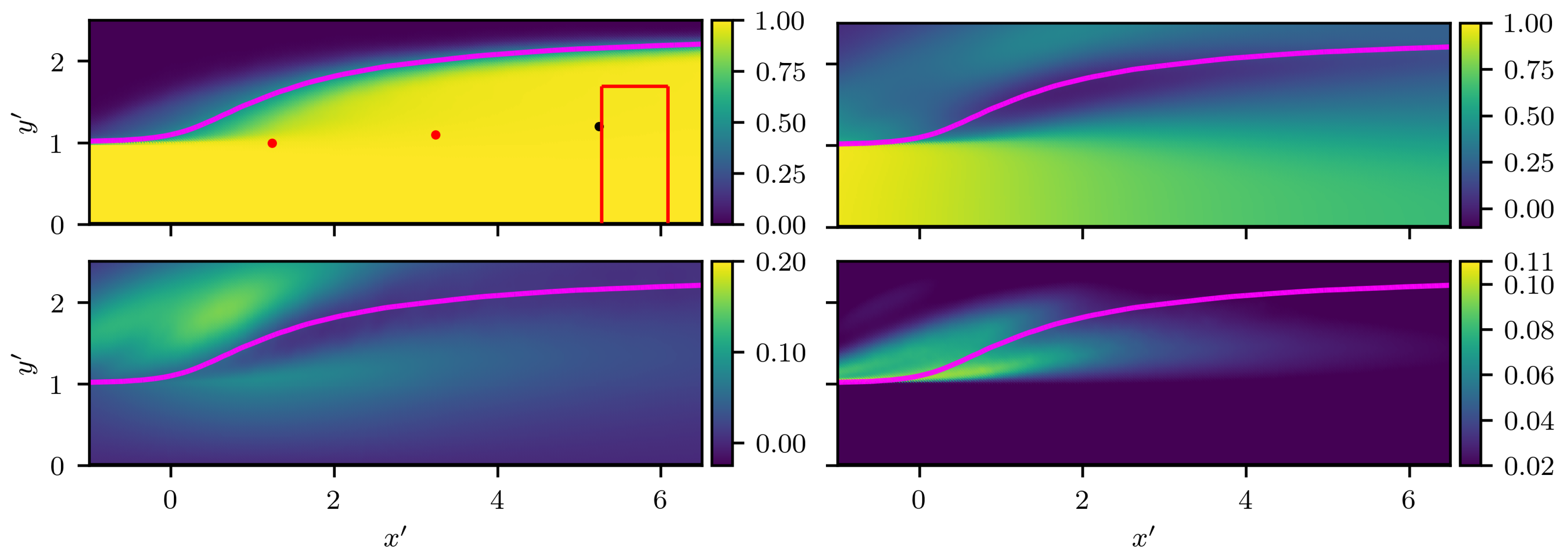
An overview of the distribution of the main flow quantities is given first; see Figure 3. The top-left plot shows the distribution of $\langle \alpha \rangle$, with the magenta line showing $\langle {\alpha }_{0.5}\rangle$. Close to the toe of the jump, and some distance downstream, the values of $\langle \alpha \rangle$ were significantly lower than one, indicating air entrainment. The mean streamwise and vertical velocities are shown in the top-right and bottom-left plots, respectively. As expected, the streamwise velocity was significantly lower downstream of the jump. It is also visible how the boundary layer in the gas followed the interface, leading to an increase in the vertical velocity in a region above the toe of the jump. Finally, the mean turbulent kinetic energy per unit mass, $\langle k\rangle$, is shown in the bottom-right plot. High values were observed in the region close to the toe, with the peak directly downstream of it. This reflects the coupling between turbulence and the air entrainment.

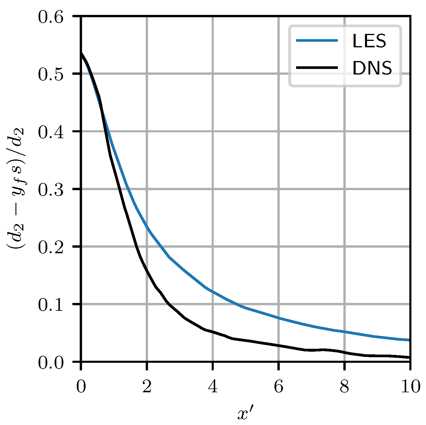
As discussed in the Introduction, the depth of the water after the jump, $d_2$, can be computed a priori. It was therefore possible to compute how the location of the interface approaches $d_2$ with increasing x. The corresponding graph is shown in Figure 4 along with the reference DNS data. We note that the value at $x^{\prime }=0$ was fixed through the definition for $x_{toe}$, which explains why the agreement with the DNS was perfect. The rate of growth of the water depth continued to be similar in both the LES and DNS up to $x^{\prime }\approx 1$. Further downstream, the DNS values converged towards $d_2$ at a faster pace, and for the LES, full convergence was in fact not achieved in the limits of the computational domain. The observed discrepancy was likely explained by the difference in the treatment of the outflow boundary.

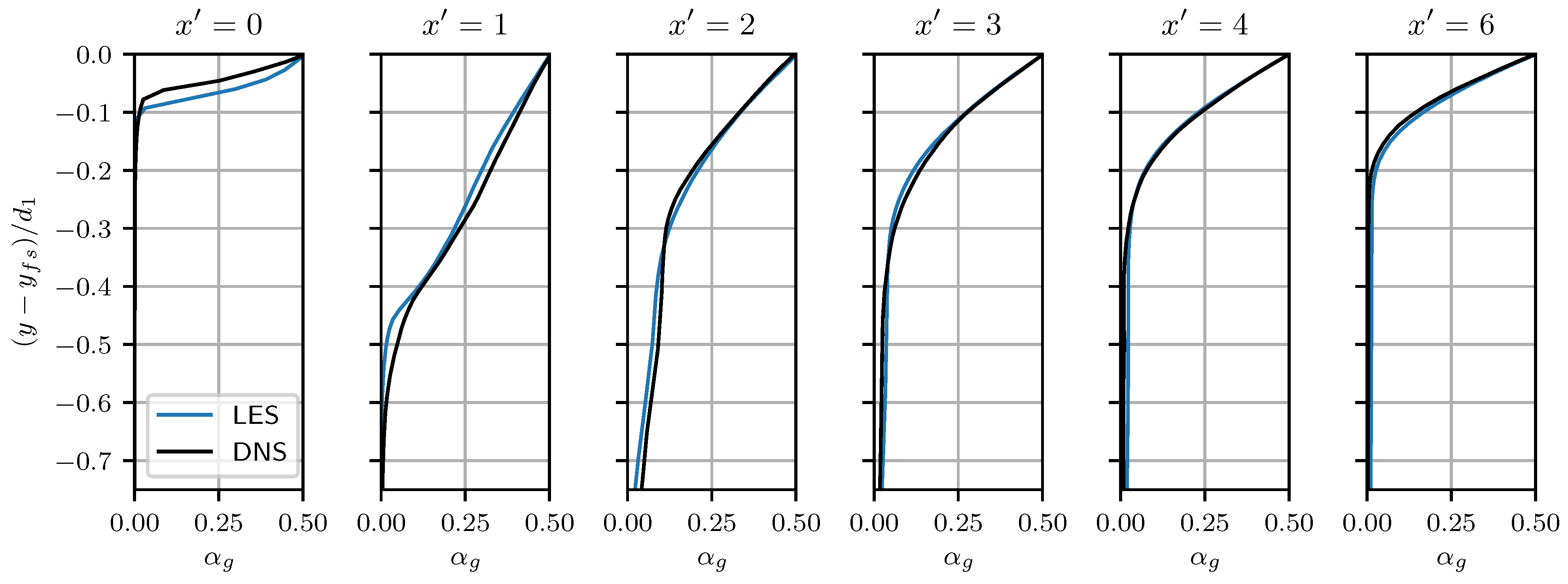
Figure 5 shows the obtained profiles of $\langle \alpha \rangle$. The agreement with the DNS was extremely good, with observable discrepancies only at $x^{\prime }=0$ and $x^{\prime }=1$. As discussed above, the most intense air entrainment occurred right downstream of the toe, so it is unsurprising that capturing the same $\langle \alpha \rangle$ profile in this region was the most difficult.

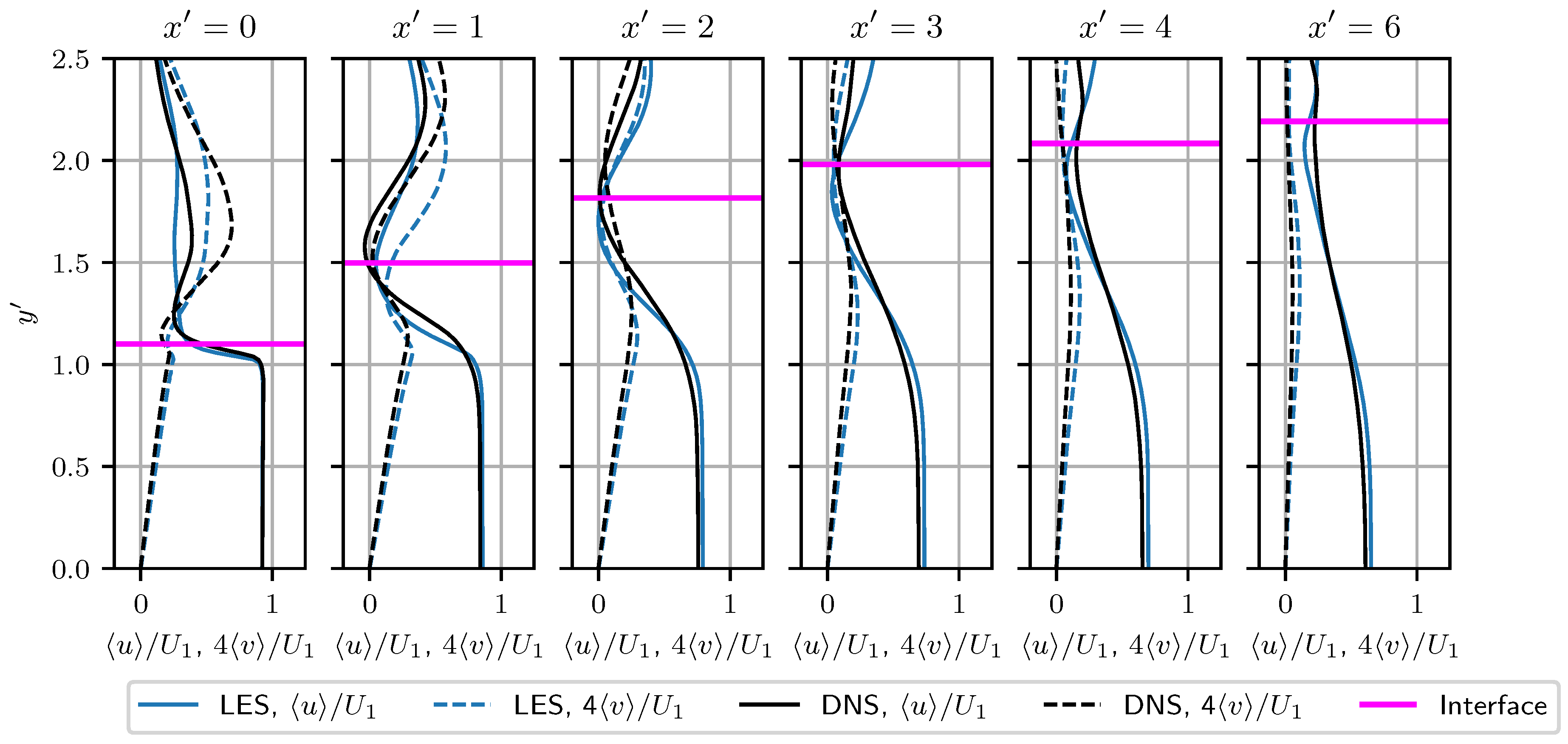
The mean streamwise and vertical velocity profiles are shown in Figure 6. The horizontal magenta lines show the positions of $\langle {\alpha }_{0.5}\rangle$. Excellent agreement with the reference was obtained at all six streamwise positions. A noticeable deviation was only observed in the values of the vertical velocity of the air, which are not of particular interest and can be significantly affected by the boundary condition at the top of the domain.

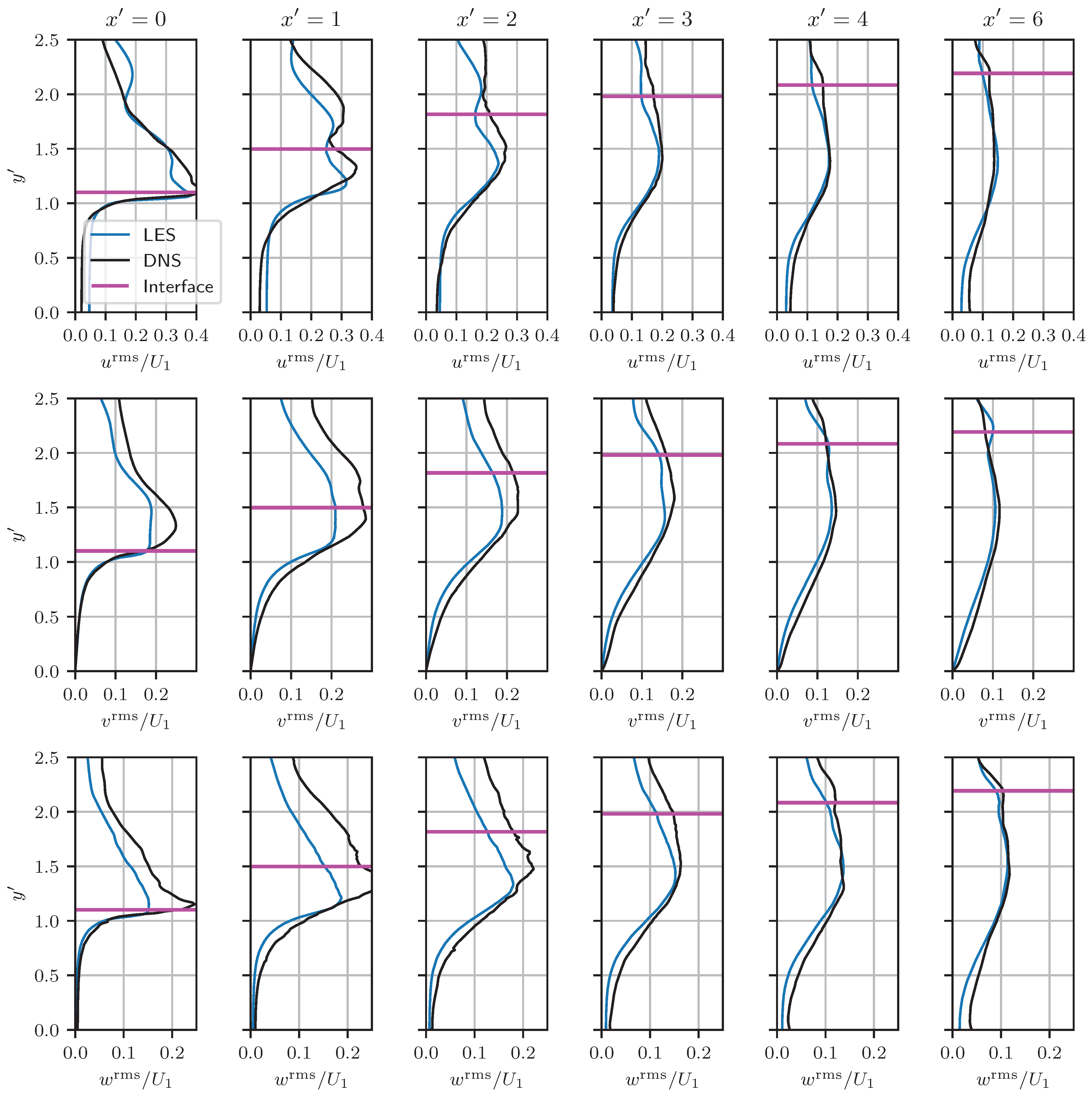
The profiles of the root-mean-squared values of the three velocity components are shown in Figure 7. We note that the inspection of the DNS data clearly showed that these second-order statistical moments did not completely converge; see Figure 8 in [4]. In light of this and the differences in the simulation setup, the obtained agreement was generally very good. All three components were predicted with a similar accuracy. It is noteworthy that the disagreement with the DNS was chiefly observed in the air and a short distance below the interface, whereas closer to the bottom, the match was close to perfect.

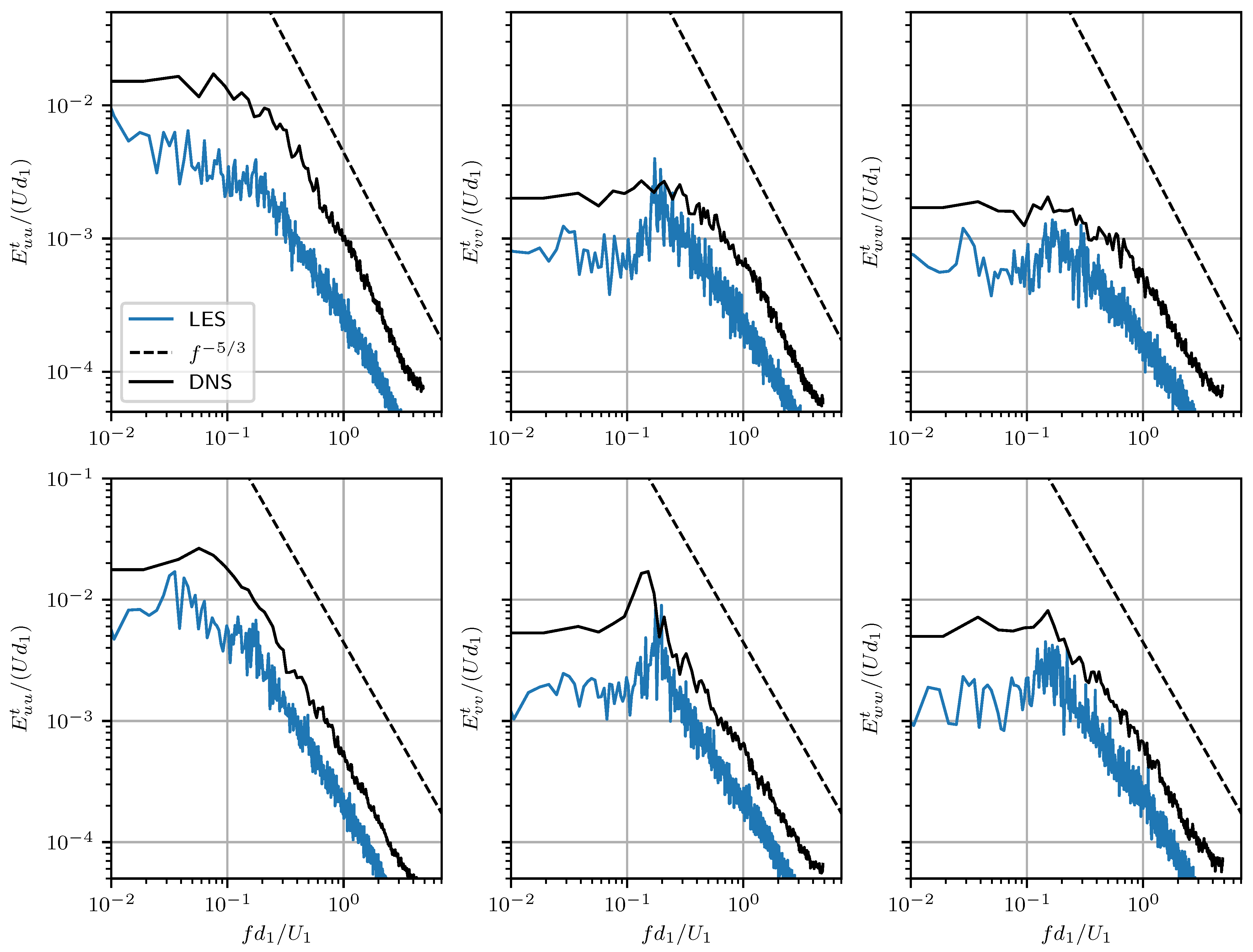
The analysis continued with the consideration of the temporal energy spectra of the velocity fluctuations. These were computed at two $[x^{\prime },y^{\prime }]$ positions: $[1.24,1]$, $[3.24,1.1]$. These are shown with red dots in the top-left plot in Figure 3. Note that the $x^{\prime }$ values were essentially an outcome of the simulation, since it was not possible to know the value of $x_{toe}$ a priori. Furthermore, the intention was to use the same x and y values in the whole simulation campaign, and the location of $x_{toe}$ varied slightly from simulation to simulation. The values were therefore chosen in a conservative way to ensure that both locations were to the right of the toe. The DNS data also provided temporal velocity spectra, including the following $[x^{\prime },y^{\prime }]$ positions: $[0,1]$, $[2,1.1]$. Both the DNS and LES data are shown in Figure 8. The LES recovered the correct slope in the inertial range, which was in most cases close to the canonical $-5/3$-power spectrum. Less energy was contained in the fluctuations in the case of the LES, but this was likely a consequence of the signals being sampled from locations further from the toe. Spectra for all three velocity components were predicted with comparable precision.

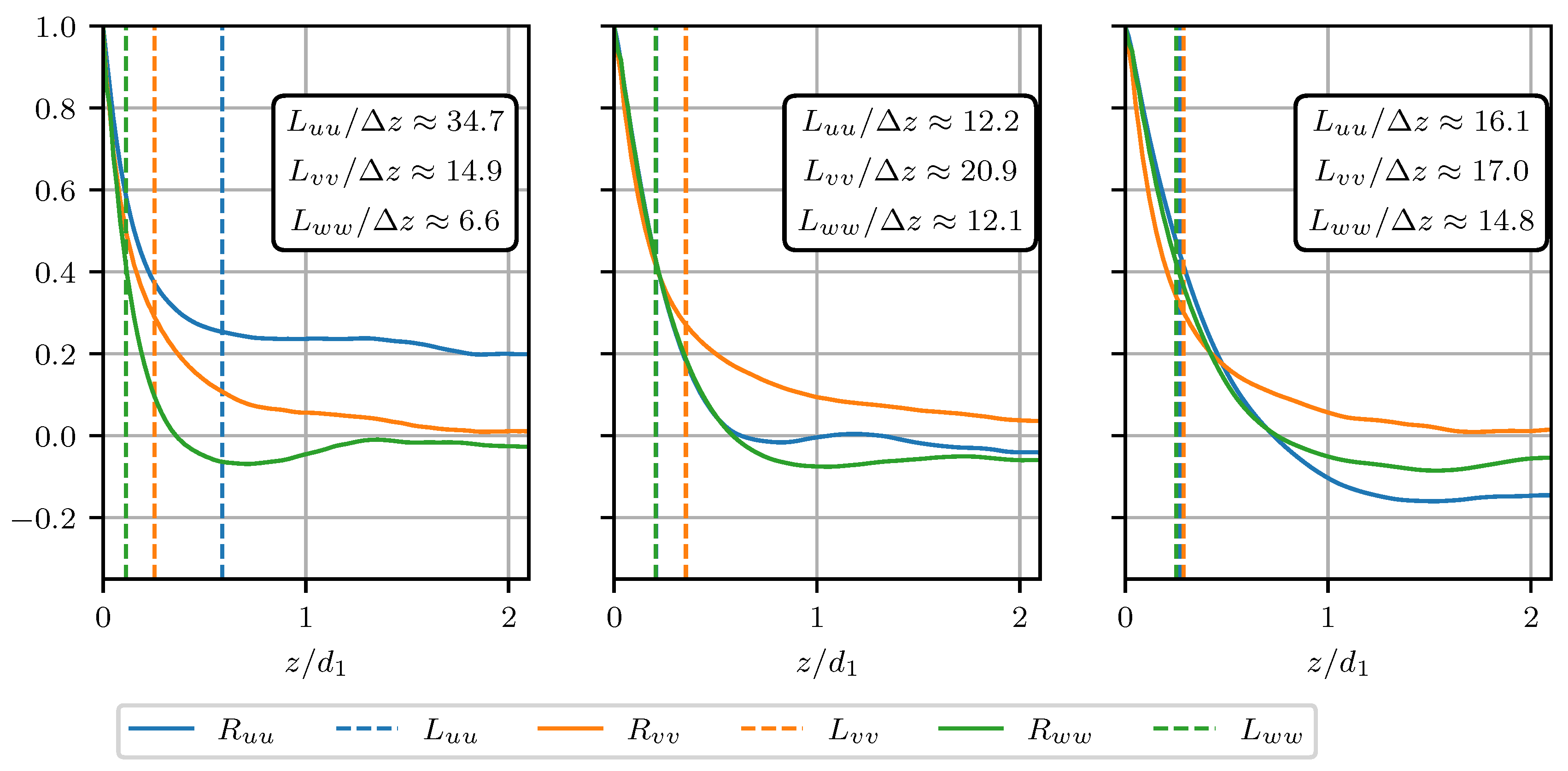
Next, the spanwise autocorrelation functions of the three velocity components, $R_{u_i{u}_i}$, were considered. These were computed at the same two $[x^{\prime },y^{\prime }]$ locations as the temporal spectra, plus an additional location further downstream: $[5.24,1]$; see the black dot in Figure 3. The result is shown in Figure 9. Evidently, $R_{uu}$, did not decline to zero for two of the three considered locations. This indicates that the spanwise dimension of the computational domain was somewhat insufficient and prompted the use of a larger domain for the simulations on the $\Delta x3$ and $\Delta x4$ meshes. The figure also presents the ratio of the integral length scales $L_{u_i{u}_i}$ and the cell size in the spanwise direction $\Delta z$. The smallest scale to be discretised was $L_{ww}$, and at $[1.24,1]$, it was only covered by $\approx 6.6$ cells. By comparison, in [33], eight cells were recommended for a coarse LES. This may indicate that even with the $\Delta x1$ mesh, some turbulent scales were resolved poorly. Alternatively, the integral length scale may be a poor metric to relate the grid resolution for this particular flow. In any case, further downstream, $L_{u_i{u}_i}$ grew, meaning that the resolution with respect to them improved.

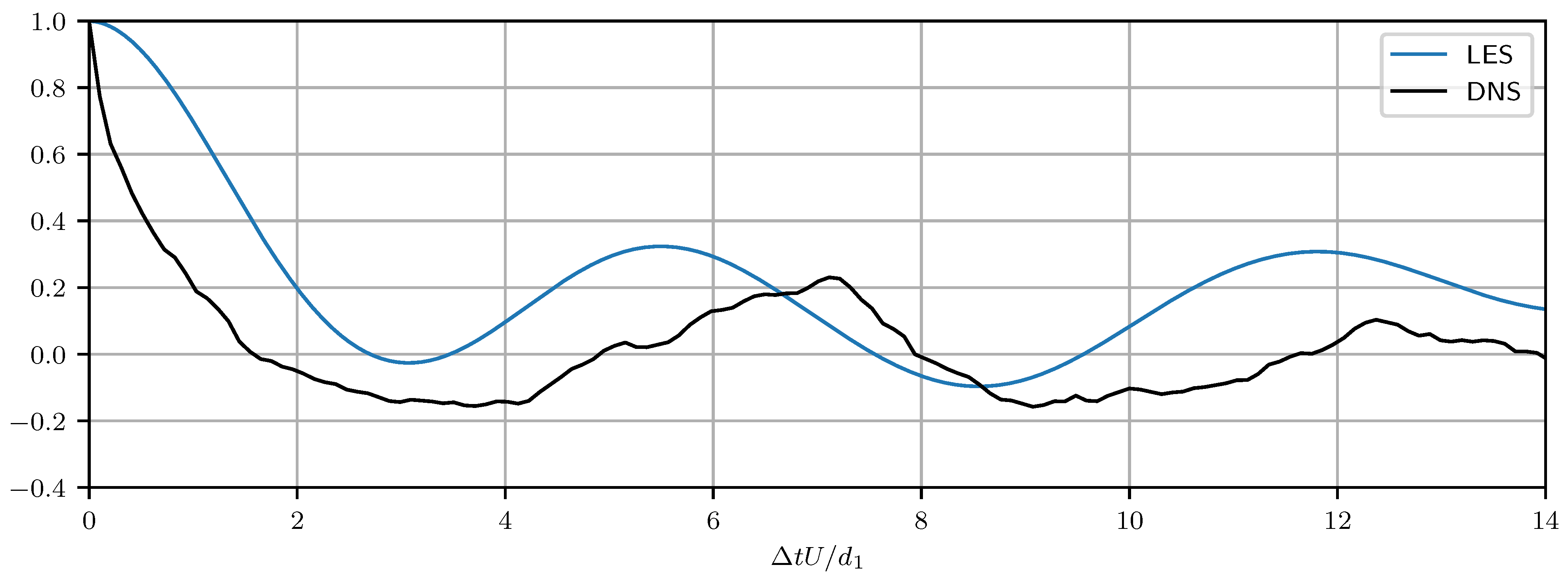
Lastly, we analysed the air entrainment by considering the temporal variation of the volume of air passing through the box $x^{\prime }\in [5.27,6.09]$, $y^{\prime }\in [0,1.70]$. The box is shown with red lines in the top-left plot in Figure 3. Similar to the analysis made for the DNS [4], we considered the autocorrelation function of the recorded signal. The result is shown in Figure 10. As expected, strong periodicity was revealed. The DNS data appeared somewhat unconverged, but the location of the first peak was relatively close to the LES. The integral time scales corresponding to the two curves were clearly different, but that is explained by the fact that the width of the box used for sampling the signal was larger in the LES.

The primary conclusion of this section is that OpenFOAM^® can be successfully used for scale-resolving simulations of the CHJ. This can probably be extended to include other codes based on the same discretisation and multiphase modelling frameworks. In spite of the slight differences in the simulation setup, the observed overall agreement with the DNS data was good not only for the first- and second-order statistical moments of the considered flow variables, but also for temporal turbulent spectra and the air entrainment properties. This justifies using the produced dataset as an accurate reference for the particular simulation setup selected.

4.3. Influence of Modelling Parameters

In this section, the effects of the grid resolution, amount of upwinding, and interface-capturing method on the cost and accuracy of the results are considered. The cost of the simulations is analysed first, and the associated metric, $N_h$, is defined as follows. First, the simulation logs were used to compute the number of physical hours necessary to advance each simulation by 1 s. Since the simulations on different grids were parallelised using different amounts of computational cores, the obtained timings were then multiplied by the corresponding amount of cores used. This assumed linear scaling of the computational effort with parallelisation, which was not exact, but provided a very good approximation in the range of core numbers used in the study. Recall also that in the simulations using isoAdvector, the time step was adjusted to ensure the maximum Courant number was $<0.5$, whereas $0.75$ was used in the MULES simulations. To be able to account for the cost difference associated with the VoF algorithm as such, the cost metric for the MULES simulations was premultiplied by $0.75/0.5$. Note that since a typical desktop computer has around 10 computational cores and the full simulation needs to be run for about 10 s, $N_h$ also gives a rough estimate of how many hours it would take to perform a given simulation on a desktop machine.

The obtained values of $N_h$ are shown in

Table 2. The simulation cost metric, $N_h$. For each $\Delta x$ and $u\%$ combination, two values are given, corresponding to MULES and isoAdvector, respectively.

	$\mathit{u}10\%$	$\mathit{u}25\%$	$\mathit{u}50\%$	$\mathit{u}100\%$
$\Delta x2$	595/825	553/855	554/778	591/801
$\Delta x3$	284/-	197/257	199/264	198/250
$\Delta x4$	75/-	53/62	52/66	50/64

. Each entry contains two numbers, corresponding to MULES and isoAdvector. It is evident that the isoAdvector simulations are more expensive. Depending on the other simulation parameters, the ratio of $N_h$ varied within $\approx [1.17$, $1.55]$. As a general trend, isoAdvector became relatively more expensive with increased mesh resolution. Numerical dissipation sometimes favourably affected the amount of iterations necessary to solve the pressure equation. Here, this effect was observed when the transition from 10% to 25% upwinding occurred, with the former always leading to a more expensive simulation. However, for higher $u\%$, the effect of dissipation on $N_h$ was neither particularly strong nor regular. Considering the cost as a function of $\Delta x$, it is crucial to recall that the $\Delta x2$ simulations were performed on a thinner domain. Since the computational effort did not scale linearly with the number of cells, this could not be directly accounted for in the metric. Based on the data, on a desktop machine, it was possible to perform $\Delta x4$ simulations in about 3 d and $\Delta x3$ in about 10 d. For $\Delta x2$, the corresponding number was from 25 d to 35 d depending on the simulation settings. Taking into account the increased access of both academia and industry to HPC hardware, it can be said that the simulations on all three grids were relatively inexpensive, at least by LES standards.

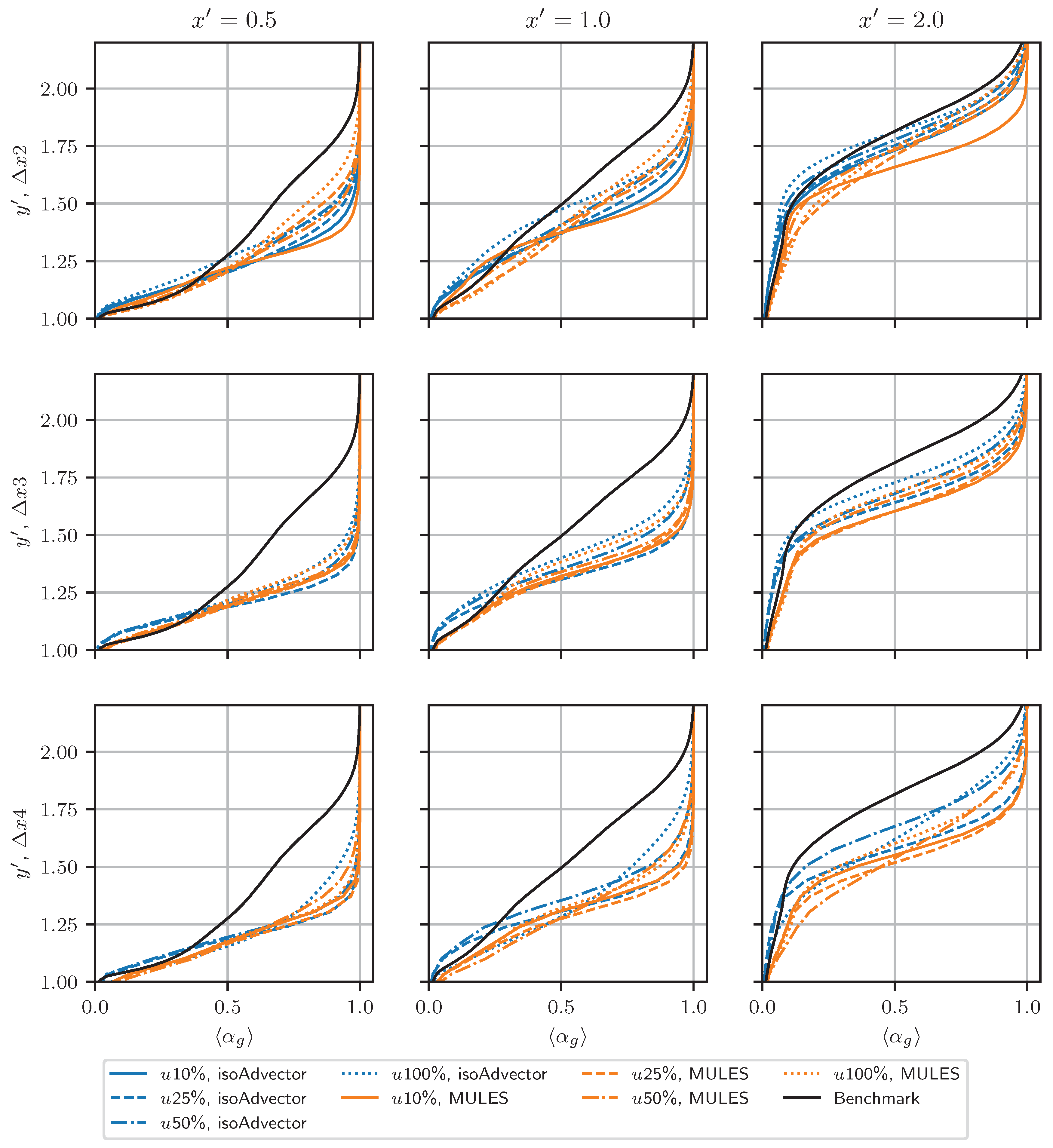
Next, the computed profiles of $\langle \alpha \rangle$ were investigated; see Figure 11. The benchmark simulation revealed that the region of the flow that was most difficult to predict was directly downstream of the toe. Therefore, here, we focused on the following streamwise positions: $x^{\prime }=0.5$, $1.0$, $2.0$. The clear trend overarching all $x^{\prime }$ and $\Delta x$ was that a higher amount of upwinding led to better results. For the majority of $\Delta x$ and streamwise positions, using isoAdvector and $u100\%$ led to the best predictive accuracy. The fact that using more dissipative schemes improved the results was somewhat unexpected, because typically, the recommendation for scale-resolving simulations is to keep dissipativity to a minimum. However, it should be appreciated that in VoF, any parasitic currents arising due to numerical errors of the dispersive type propagate into errors in the advection of the interface. It appears that avoiding these errors is more important than resolving steep velocity gradients. As expected, the quality of the results degraded with the coarsening of the mesh. The most precise result on $\Delta x2$ was quite close to the benchmark. On the coarser grids, the accuracy was acceptable considering how inexpensive the corresponding simulations were.

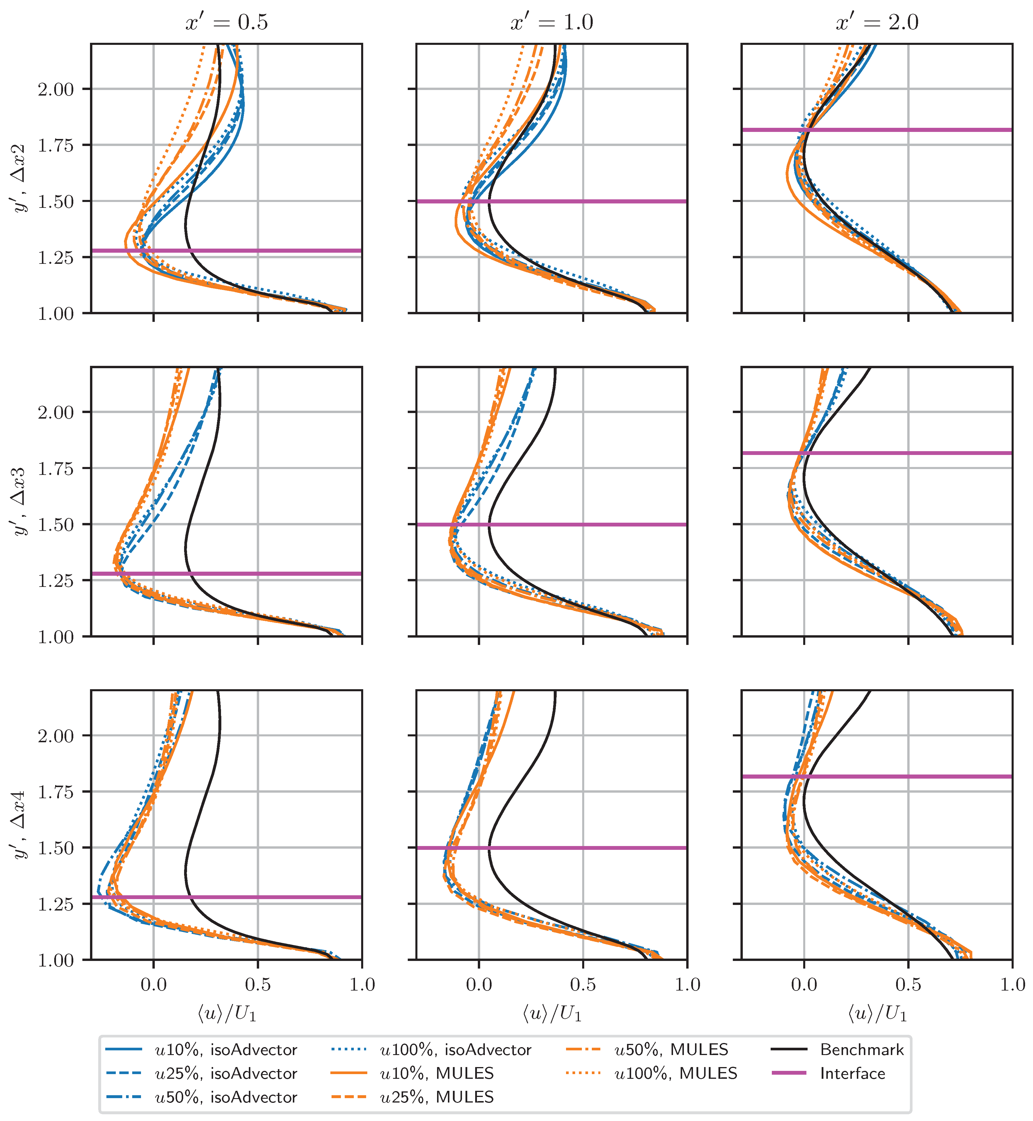
The predictions of the mean velocity are analysed next; see Figure 12. We focused on the streamwise component $\langle u\rangle$ only, since the level of accuracy of $\langle v\rangle$ was similar. It was clear that compared to $\langle \alpha \rangle$, the results were more robust with respect to the amount of upwinding. This is rather peculiar: the choice of interpolation scheme for u had little effect on $\langle u\rangle$, but a stronger effect on a different quantity, $\langle \alpha \rangle$. Nevertheless, the profiles obtained with higher $u\%$ were generally slightly more accurate, at least in the water phase. Using isoAdvector led to superior accuracy in the gas phase, whereas in the water phase, no significant advantage over MULES was achieved. The combination of $\Delta x2$, $u100\%$, and isoAdvector gave the best results, which were close to the benchmark. At coarser resolutions, the accuracy deteriorated, but not as strongly as for $\langle \alpha \rangle$.

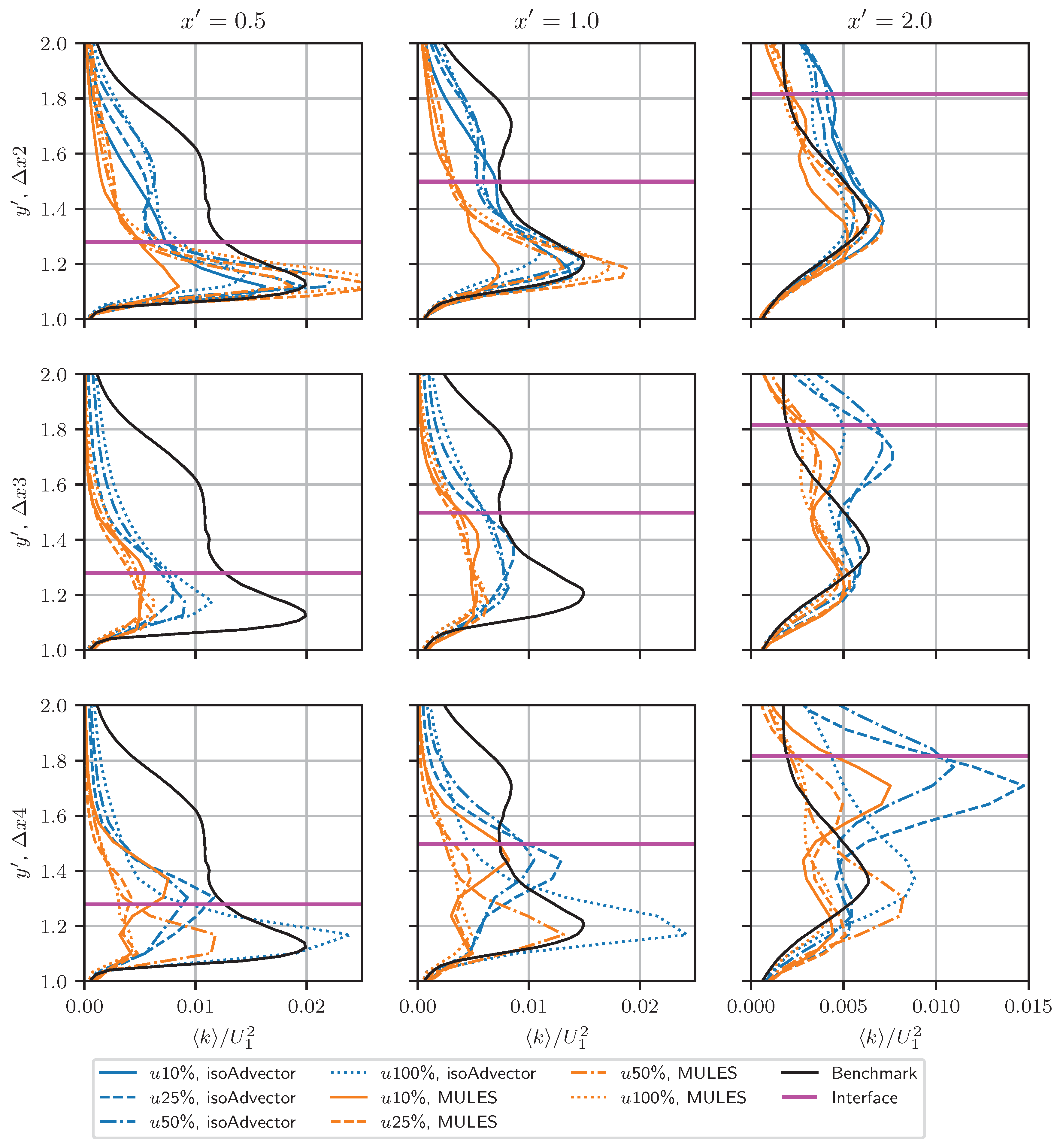
Figure 13 shows the obtained profiles of $\langle k\rangle$. The observed error patterns were significantly less regular than in $\langle u\rangle$ and $\langle \alpha \rangle$. Two factors contributed to this. One is that $\langle k\rangle$ lumped together the errors in the variances of the three velocity components. The other was that parasitic oscillations had a direct amplifying effect on $\langle k\rangle$. Both of the above can lead to either error cancellation or amplification. On the $\Delta x2$ grid, the best results were achieved with isoAdvector and 25/50% upwinding. In the case of $u100\%$, the main peak in the detached shear layer was somewhat under-predicted, but the discrepancy was not very significant. An interesting observation is that at lower grid resolutions, a secondary peak in $\langle k\rangle$ was developed for $x^{\prime }=1.0$ and $2.0$ right underneath the interface. This unphysical peak was more pronounced when isoAdvector was used and could even be observed on the $\Delta x2$ grid when this interface-capturing technique was used. It was present in all three components of the velocity variance, although for the streamwise component, it was less pronounced. The size of the peak grew with a decreasing amount of upwinding, which confirmed its numerical origin. Even apart from this additional peak, the results for $\langle k\rangle$ on $\Delta x3$ and $\Delta x4$ were quite inaccurate, although the combination $\Delta x4$, $u50\%$, and MULES reproduced the main features of the benchmark profiles fairly faithfully.

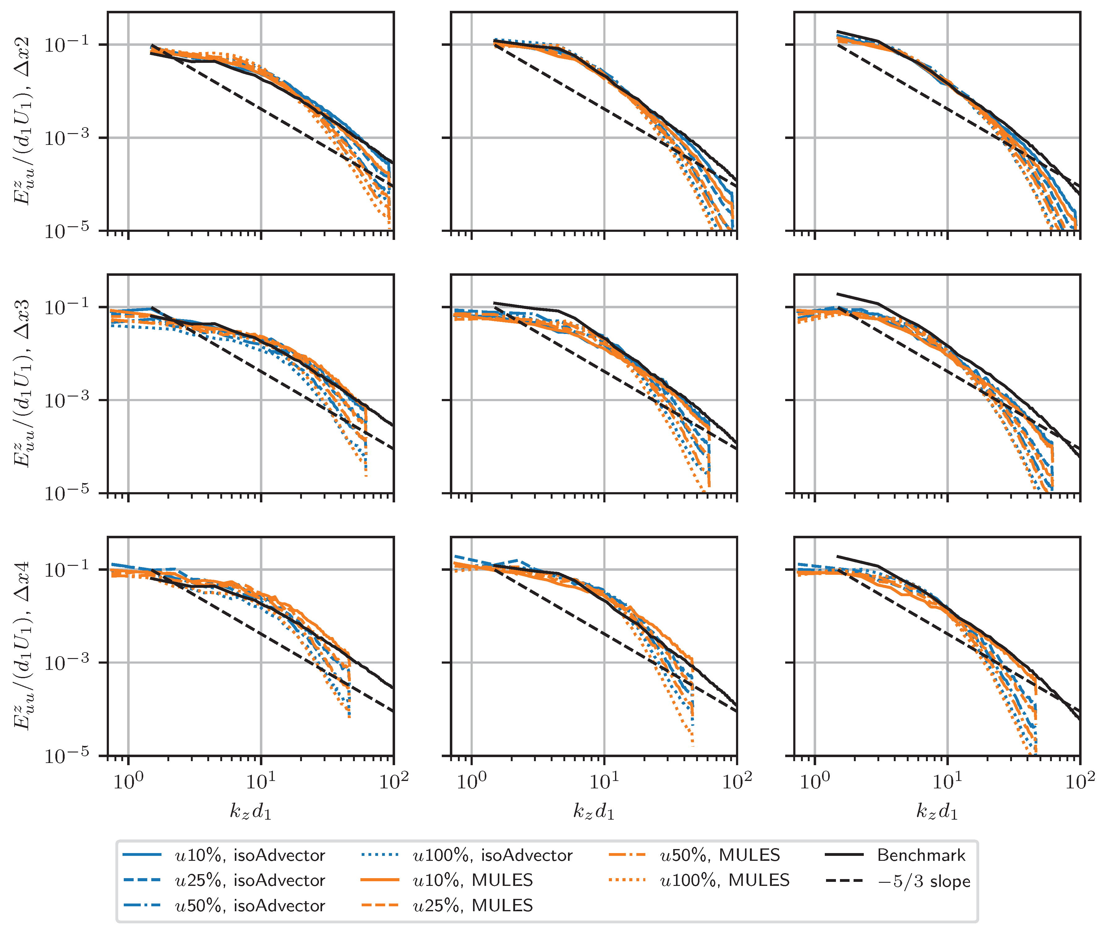
The analysis of the velocity predictions is now concluded by considering the spanwise energy spectra of the streamwise velocity; see Figure 14. The spectra were computed at the same three $[x,y]$ locations as the spanwise autocorrelation functions for the benchmark simulations. This entailed that the respective $x^{\prime }$ values were slightly different from simulation to simulation. The reason for considering spanwise spectra instead of temporal was that, due to a larger amount of samples to average across, the spanwise spectra were much smoother, making it easier to distinguish the profiles from different simulations in the plots. Unsurprisingly, increased upwinding led to heavier dampening of the high-frequency fluctuations. Due to the log–log scale being used, it was actually difficult to distinguish any effects of the VoF algorithm or $\Delta x$, besides the fact that the frequency band of the spectrum was larger for denser meshes. One could say that for small amounts of $u\%$, the spectrum was relatively well predicted even at $\Delta x4$. Therefore, one should exercise caution when making judgements regarding the mesh resolution based on the spectrum predictions.

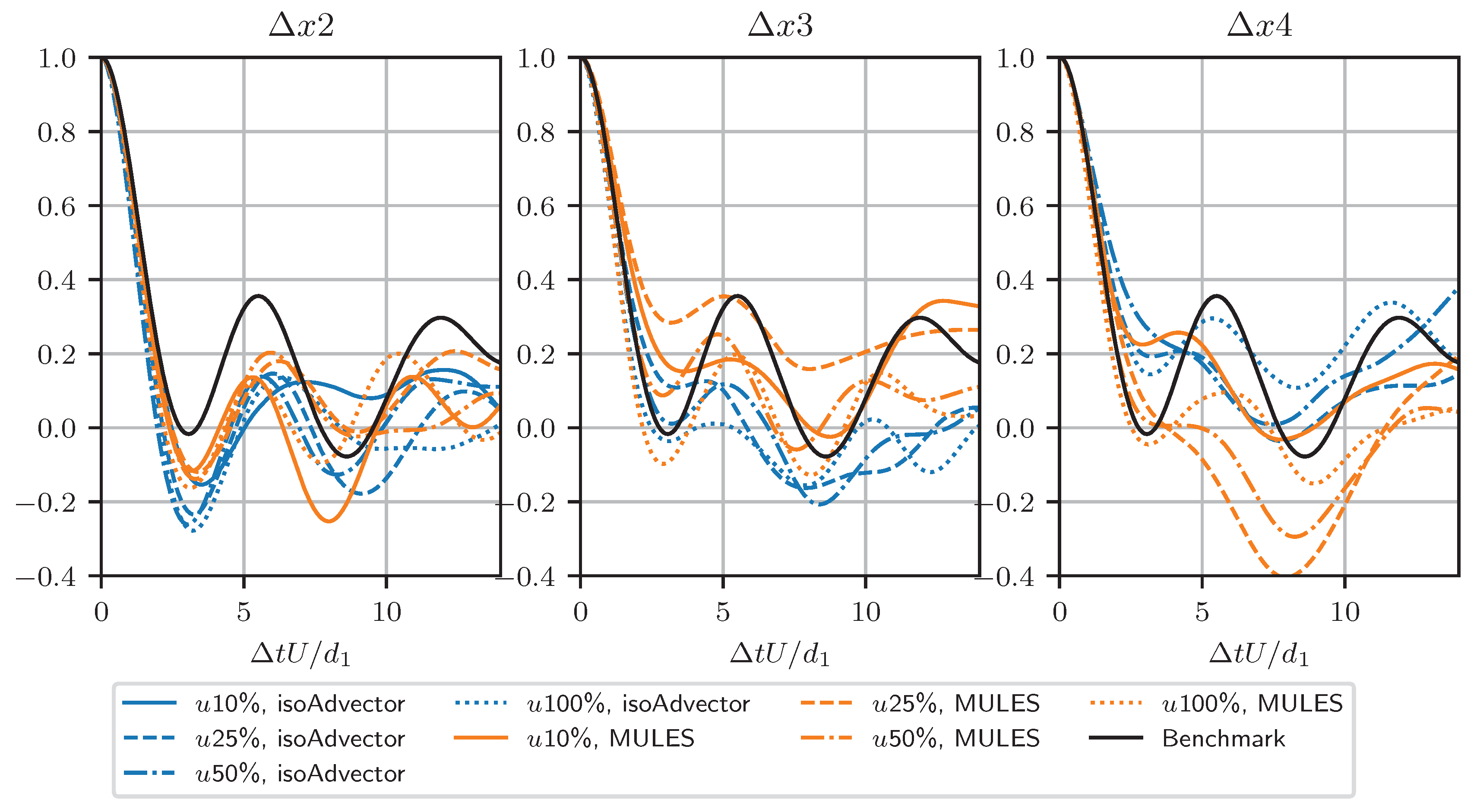
Finally, the periodicity of air entrainment was analysed. As for the benchmark simulation, the autocorrelation functions of the volume of air passing through a box located some distance downstream of the toe (see the top-left plot in Figure 3) were computed. The results are shown in Figure 15. For $\Delta x2$ and $\Delta x3$, the location of the first peak was quite well predicted by all the simulations, whereas for $\Delta x4$, the accuracy deteriorated, in particular for some of the simulations using MULES. Animations of the $\alpha =0.5$ isosurface revealed that isoAdvector did a much better job at preserving the sharpness of the interface as the entrained bubbles travelled downstream. Therefore, if tracking the fate of the bubbles is important, using this VoF approach is recommended. It should also be noted that while all the simulation predicted similar entrainment frequencies, other statistical air entrainment properties did not agree equally well. For example, the mean amount of air within the monitored box was highly affected by the choice of the VoF method, with MULES giving systematically higher values.

5. Conclusions

This article presented the results from an extensive simulation campaign studying the effects of different modelling parameters on the accuracy of LES of CHJ flow at ${\mathrm{Fr}}_1=2$. The simulations were performed with a general-purpose finite-volume-based CFD code, making the obtained results relevant for industry professionals and researches alike.

A benchmark simulation on a dense grid was conducted to test whether commonly employed VoF-based multiphase modelling methodologies are sufficiently accurate to capture the complicated physics of the flow. The comparison with the DNS data [4] showed that the answer was positive, and good agreement with the reference was found for the considered quantities of interest. However, it was also revealed that numerical instabilities, discussed in Section 2.5, constituted a significant problem. It was virtually impossible to know a priori whether the chosen numerical setup would lead to a stable simulation, and a crash may occur sporadically after a significant part of the simulation time has already past. Addressing the primary sources of instability (surface tension, density gradient term in (1)) should therefore be a high priority for the development of VoF solvers in OpenFOAM^® and other codes based on similar algorithms.

The rest of the simulation campaign focused on the effects of the grid resolution, amount of upwinding, and VoF methodology. One of the most interesting results was that the most dissipative scheme, $u100\%$, led to the best results for nearly all the considered quantities of interest. This represents another example of how multiphase simulations can react counter-intuitively with respect to a change in the computational algorithm. It appeared that, for volume fraction transfer, ensuring the lack of strong dispersive errors was for this case more important than minimizing the numerical dissipation. Fortunately, dissipation also favours stability, which means that having both an accurate and stable numerical setup is possible.

Using the geometric VoF methodology, isoAdvector, led to improved interface sharpness and thus improved the resolution of entrained bubbles. The improvement in the accuracy of averaged flow quantities compared to MULES was however, not so strong, and for selected quantities and streamwise locations, MULES actually gave better results. The chance of instability was also increased by isoAdvector, and for some combinations of modelling parameters, the simulations could not be run. Unfortunately, this included the benchmark simulation. The computational costs of isoAdvector simulations were also significantly larger than their MULES counterparts; see Table 2. For equivalent simulation settings, the maximum cost ratio was 1.5; however, due to MULES being more stable, it is possible to select a larger time step, which would make the difference even larger. It is thus recommended to use isoAdvector when tracking the fate of individual air bubbles is particularly important.

The grid resolution appeared to be the most significant factor when it came to the predictive accuracy. The sensitivity was particularly strong right downstream of the toe, for which even the $\Delta x2$ grid gave relatively poor results. However, further downstream, the loss of accuracy quickly decreased. The $\Delta x3$ grid could be used to reduce the costs significantly and still maintain a level of predictive accuracy that can be suitable for industrial simulations. Using the $\Delta x4$ can only be recommended when the CHJ is a part of a larger flow configuration and is not of particular interest as such.

References

1. Bayon-Barrachina, A.; Lopez-Jimenez, P.A. Numerical analysis of hydraulic jumps using OpenFOAM. J. Hydroinform. 2015, 17, 662–678. [Google Scholar] [CrossRef] [Green Version]
2. Valero, D.; Viti, N.; Gualtieri, C. Numerical simulation of hydraulic jumps. Part 1: Experimental data for modelling performance assessment. Water 2018, 11, 36. [Google Scholar] [CrossRef] [Green Version]
3. Valero, D.; Viti, N.; Gualtieri, C. Numerical simulation of hydraulic jumps. Part 2: Recent results and future outlook. Water 2018, 11, 28. [Google Scholar] [CrossRef] [Green Version]
4. Mortazavi, M.; Le Chenadec, V.; Moin, P.; Mani, A. Direct numerical simulation of a turbulent hydraulic jump: Turbulence statistics and air entrainment. J. Fluid Mech. 2016, 797, 60–94. [Google Scholar] [CrossRef]
5. Chanson, H. The Hydraulics of Open Channel Flow: An Introduction; Elsevier: Burlington, MA, USA, 2004; p. 601. [Google Scholar]
6. Jain, S.C. Open-Channel Flow; Wiley: Hoboken, NJ, USA, 2001; p. 328. [Google Scholar]
7. Kundu, P.K.; Cohen, I.M. Fluid Mechanics, 4th ed.; Academic Press: Burlington, MA, USA, 2008. [Google Scholar]
8. Retsinis, E.; Papanicolaou, P. Numerical and experimental study of classical hydraulic jump. Water 2020, 12, 1766. [Google Scholar] [CrossRef]
9. Ma, J.; Oberai, A.A.; Lahey, R.; Drew, D.A. Modeling air entrainment and transport in a hydraulic jump using two-fluid RANS and DES turbulence models. Heat Mass Transf. 2011, 47, 911–919. [Google Scholar] [CrossRef]
10. Jesudhas, V.; Balachandar, R.; Roussinova, V.; Barron, R. Turbulence characteristics of classical hydraulic jump using DES. J. Hydraul. Eng. 2018, 144, 04018022. [Google Scholar] [CrossRef]
11. Jesudhas, V.; Balachandar, R.; Wang, H.; Murzyn, F. Modelling hydraulic jumps: IDDES versus experiments. Environ. Fluid Mech. 2020, 20, 393–413. [Google Scholar] [CrossRef]
12. Gonzalez, A.; Bombardelli, F.A. Two-phase-flow theoretical and numerical models for hydraulic jumps, including air entrainment. In Proceedings of the 31st IAHR Congress, Seoul, Korea, 11–16 September 2005. [Google Scholar]
13. Lubin, P.; Glockner, S.; Chanson, H. Numerical simulation of air entrainment and turbulence in a hydraulic jump. In Proceedings of the Colloque SHF: Modeles Physiques Hydrauliques, Lyon, France, 24–25 November 2009; pp. 109–114. [Google Scholar]
14. Hirt, C.W.; Nichols, B.D. Volume of Fluid (VOF) method for the dynamics of free boundaries. J. Comput. Phys. 1981, 39, 201–225. [Google Scholar] [CrossRef]
15. Brackbill, J.U.; Kothe, D.B.; Zemach, C. A continuum method for modeling surface tension. J. Comput. Phys. 1992, 100, 335–354. [Google Scholar] [CrossRef]
16. Damián, S.M. An Extended Mixture Model for the Simultaneous Treatment of Short and Long Scale Interfaces. Ph.D. Thesis, National University of the Littoral, Santa Fe, Argentina, 2013. [Google Scholar]
17. Zalesak, S.T. Fully multidimensional flux-corrected transport algorithms for fluids. J. Comput. Phys. 1979, 31, 335–362. [Google Scholar] [CrossRef]
18. Roenby, J.; Bredmose, H.; Jasak, H. A computational method for sharp interface advection. R. Soc. Open Sci. 2016, 3, 160405. [Google Scholar] [CrossRef] [PubMed] [Green Version]
19. Issa, R.I. Solution of the implicitly discretised fluid flow equations by operator-splitting. J. Comput. Phys. 1986, 62, 40–65. [Google Scholar] [CrossRef]
20. Rusche, H. Computational Fluid Dynamics of Dispersed Two-Phase Flows at High Phase Fractions. Ph.D. Thesis, Imperial College of Science, Technology and Medicine, London, UK, 2002. [Google Scholar]
21. Versteeg, H.K.; Malalasekera, W. An Introduction to Computational Fluid Dynamics: The Finite Volume Method, 2nd ed.; Pearson Education Limited: Essex, UK, 2007. [Google Scholar]
22. Nicoud, F.; Ducros, F. Subgrid-scale stress modelling based on the square of the velocity gradient tensor. Flow Turbul. Combust. 1999, 62, 183–200. [Google Scholar] [CrossRef]
23. Mukha, T. Inflow Generation for Scale-Resolving Simulations of Turbulent Boundary Layers; Uppsala University: Uppsala, Sweden, 2016. [Google Scholar]
24. Cano-Lozano, J.C.; Bolaños-Jiménez, R.; Gutiérrez-Montes, C.; Martínez-Bazán, C. The use of Volume of Fluid technique to analyze multiphase flows: Specific case of bubble rising in still liquids. Appl. Math. Model. 2015, 39, 3290–3305. [Google Scholar] [CrossRef]
25. Scheufler, H. Implementation of new surface tension models for the Volume of Fluid Method. In Proceedings of the 7th ESI OpenFOAM Conference, Berlin, Germany, 15–17 October 2019. [Google Scholar]
26. Popinet, S. An accurate adaptive solver for surface-tension-driven interfacial flows. J. Comput. Phys. 2009, 228, 5838–5866. [Google Scholar] [CrossRef] [Green Version]
27. Gamet, L.; Scala, M.; Roenby, J.; Scheufler, H.; Pierson, J.L. Validation of volume-of-fluid OpenFOAM® isoAdvector solvers using single bubble benchmarks. Comput. Fluids 2020, 213, 104722. [Google Scholar] [CrossRef]
28. Scheufler, H.; Roenby, J. TwoPhaseFlow: An OpenFOAM based framework for development of two phase flow solvers. arXiv 2021, arXiv:2103.00870. [Google Scholar]
29. Vukčević, V.; Jasak, H.; Gatin, I. Implementation of the Ghost Fluid Method for free surface flows in polyhedral Finite Volume framework. Comput. Fluids 2017, 153, 1–19. [Google Scholar] [CrossRef]
30. Witt, A.; Gulliver, J.; Shen, L. Simulating air entrainment and vortex dynamics in a hydraulic jump. Int. J. Multiph. Flow 2015, 72, 165–180. [Google Scholar] [CrossRef] [Green Version]
31. Witt, A.; Gulliver, J.S.; Shen, L. Numerical investigation of vorticity and bubble clustering in an air entraining hydraulic jump. Comput. Fluids 2018, 172, 162–180. [Google Scholar] [CrossRef]
32. Bayon, A.; Valero, D.; García-Bartual, R.; Vallés-Morán, F.J.; López-Jiménez, P.A. Performance assessment of OpenFOAM and FLOW-3D in the numerical modeling of a low Reynolds number hydraulic jump. Environ. Model. Softw. 2016, 80, 322–335. [Google Scholar] [CrossRef]
33. Davidson, L. Large Eddy Simulations: How to evaluate resolution. Int. J. Heat Fluid Flow 2009, 30, 1016–1025. [Google Scholar] [CrossRef] [Green Version]
Figure 1. Classical hydraulic jump at F r 1 = 2 ; a snapshot of the air–water interface.
Fluids 07 00101 g001
Figure 2. Simulation setup.
Fluids 07 00101 g002
Figure 3. Distribution of α (top left), u / U 1 (top right), v / U 1 (bottom left), and k / U 1 2 (bottom right) in the benchmark simulation. The magenta line shows α 0.5 .
Fluids 07 00101 g003
Figure 4. Convergence of the interface height towards d 2 in the benchmark simulation.
Fluids 07 00101 g004
Figure 5. The profiles of α in the benchmark simulation.
Fluids 07 00101 g005
Figure 6. The profiles of u (solid lines) and 4 v (dashed lines) obtained in the benchmark simulation. The magenta line shows the location of the interface.
Fluids 07 00101 g006
Figure 7. The profiles of u r m s / U 1 , v r m s / U 1 , and w r m s / U 1 obtained in the benchmark simulation. The magenta line shows the location of the interface.
Fluids 07 00101 g007
Figure 8. Temporal energy spectra of the three components of velocity at two selected [ x , y ] positions: [ 1.24 , 1 ] (top); [ 3.24 , 1.1 ] (bottom).
Fluids 07 00101 g008
Figure 9. Spanwise two-point auto-correlations of velocity components computed at 3 selected [ x , y ] locations: [ 1.24 , 1 ] (left); [ 3.24 , 1.1 ] (middle); [ 5.24 , 1 ] (right). Vertical dashed lines show the integral length scales.
Fluids 07 00101 g009
Figure 10. Autocorrelation function of the time signal of the air volume passing through the box x [ 5.27 , 6.09 ] , y [ 0 , 1.70 ] .
Fluids 07 00101 g010
Figure 11. The profiles of α obtained in the simulation campaign.
Fluids 07 00101 g011
Figure 12. The profiles of u / U 1 obtained in the simulation campaign.
Fluids 07 00101 g012
Figure 13. The profiles of k / U 1 2 obtained in the simulation campaign.
Fluids 07 00101 g013
Figure 14. The spanwise velocity spectra obtained in the simulations at three selected locations: [ 1.24 , 1 ] (left); [ 3.24 , 1.1 ] (middle); [ 5.24 , 1.4 ] (right).
Fluids 07 00101 g014
Figure 15. The obtained autocorrelation functions of the volume of leaked air.
Fluids 07 00101 g015