Simple Summary
It is too costly to compute the time advancement of many turbulent flows because the range of relevant motions is very broad and encompassing all of them is unaffordable. The typical compromise is to omit the smallest motions, replacing them by estimates of their effects, but this is not always adequate. Instead, it is proposed to fully resolve the flow advancement along selected line segments within the flow volume and to couple these segments so that the resulting formulation adequately represents all scales of motion. The modeling needed to implement this is described and the overall approach, termed autonomous microstructure evolution, is assessed conceptually and with reference to demonstrated capabilities of related methods.
Abstract
A multiscale modeling concept for numerical simulation of multiphysics turbulent flow utilizing map-based advection is described. The approach is outlined with emphasis on its theoretical foundations and physical interpretations in order to establish the context for subsequent presentation of the associated numerical algorithms and the results of validation studies. The model formulation is a synthesis of existing methods, modified and extended in order to obtain a qualitatively new capability. The salient feature of the approach is that time advancement of the flow is fully resolved both spatially and temporally, albeit with modeled advancement processes restricted to one spatial dimension. This one-dimensional advancement is the basis of a bottom-up modeling approach in which three-dimensional space is discretized into under-resolved mesh cells, each of which contains an instantiation of the modeled one-dimensional advancement. Filtering is performed only to provide inputs to a pressure correction that enforces continuity and to obtain mesh-scale-filtered outputs if desired. The one-dimensional advancement, the pressure correction, and coupling of one-dimensional instantiations using a Lagrangian implementation of mesh-resolved volume fluxes is sufficient to advance the three-dimensional flow without time advancing coarse-grained equations, a feature that motivates the designation of the approach as autonomous microscale evolution (AME). In this sense, the one-dimensional treatment is not a closure because there are no unclosed terms to evaluate. However, the approach is additionally suitable for use as a subgrid-scale closure of existing large-eddy-simulation methods. The potential capabilities and limitations of both of these implementations of the approach are assessed conceptually and with reference to demonstrated capabilities of related methods.
1. Introduction
To extend the range of applicability of numerical simulation of turbulent flows beyond the limits of affordable direct numerical simulation (DNS), under-resolved simulations with physically or algorithmically based subgrid-scale (SGS) closures are widely used, typically within the large-eddy-simulation (LES) framework. For constant-property flow, the main role of the SGS closure of LES is to dissipate kinetic energy at the physically correct rate based on the flow state. A secondary process that is important in some circumstances is the transfer of kinetic energy from unresolved scales to the LES-resolved flow solution, and accordingly, modeling of this backscatter has been incorporated into SGS closures. The resulting two-way coupling is especially important when LES is extended from constant-property flow to multiphysics flow involving combinations of buoyancy, multiphase couplings, and velocity divergence due to, for example, thermochemical processes.
Here, an approach designed to capture these and other multiphysics effects within SGS closures for LES is described. Unlike typical parameterizations, it involves idealized but physically based treatments of SGS advective and diffusive transport and other SGS processes, such as those mentioned. The approach involves DNS-level resolution of spatial structure and flow unsteadiness, which increases its cost relative to parameterizations, but it is less costly than DNS because this fine resolution is restricted to representative lines of sight within individual LES control volumes (CVs). Cost is further mitigated to the extent that the fidelity of the SGS closure allows coarsening of the LES mesh while maintaining the needed level of accuracy.
The method used for SGS closure involves one-dimensional turbulence (ODT), a form of map-based stochastic advection that has been used previously for SGS closure of LES as well as in various standalone applications, as cited below. Here, an ODT-based SGS closure is formulated that draws upon previously reported formulations but also introduces various novel elements, whose details and physical interpretations are the main focus of the present contribution.
To begin, it is important to clarify what it means to close an LES using ODT. Suppose that exact underlying DNS-level data are available at all times in all LES CVs. Then the unclosed terms in the LES equations can be evaluated exactly, yielding a fully accurate closure. However, if the LES time advances an SGS kinetic-energy equation, then the DNS data might be used to close an unclosed term in that equation. This might not be an optimal use of the DNS data, but if the available data were inexact rather than exact, then they might turn out to be more useful for closing a model equation carried by the LES rather than for closing the unclosed terms obtained by filtering the exact equation. For reacting flows, a related example is use of the data either to close the filtered chemical state or to provide the LES with reaction rates that are used to time advance filtered, hence modeled, chemical-kinetic equations.
ODT, in this context, provides surrogate DNS data that can be used to close either the filtered, but not otherwise modeled, LES equations or unclosed terms in submodels appended to these equations. Development and demonstration of either type of closure involves many choices with regard to mesh geometry, filtering technique, numerical algorithms, application cases, etc., ultimately resulting in the evaluation of only one or a few of the many options.
For the present purpose of introducing the general concepts and physical modeling approaches on which any particular modeling instantiation would be based, the following approach is adopted here. It is shown how ODT can be formulated so that, with suitable large-scale input, its time advancement can provide a local flow solution that, when filtered, is a physically plausible surrogate of the updated local filtered velocity that would otherwise be evaluated by advancing the filtered momentum equation. Thus, as an alternative to advancement of that equation, the updated filtered flow field can be obtained by time advancing and then filtering the fully resolved flow state on each ODT domain. There is one ODT domain per CV of the coarse-grained mesh, so this procedure updates the entire filtered flow field.
With the introduction of a pressure projection that adjusts the filtered flow field so as to enforce continuity, this approach becomes a self-contained ODT-based low-Mach-number flow simulation. It is a bottom-up approach that treats the evolving ODT state as the physical flow solution, albeit modeled rather than exact, that can be filtered to obtain an LES-like coarse-grained velocity field. In this context, the coarse-grained pressure is an auxiliary field that communicates large-scale information to each ODT domain, where this information reflects the collective interactions among the ODT domains and the inflow, outflow, and boundary conditions. Owing to the absence of any time advancement of the filtered velocity field, this formulation is not LES per se, so it is more appropriately termed autonomous microscale evolution (AME).
It is shown here that AME is a potentially viable alternative to LES. Its capabilities and limitations in this regard are assessed, subject to more definitive future evaluation by means of numerical implementation and model validation studies. As noted, the assessment also addresses points relevant to ODT SGS closure of LES. In what follows, operations on filtered fields are generically termed LES processes in order to discuss them in a familiar context until sufficient information specific to AME is provided so that discussion of AME becomes meaningful.
2. Overview of the Approach
2.1. ODT
In this section, the proposed SGS formulation of ODT is outlined to a sufficient extent that its coupling to other parts of the time-advancement cycle can be explained. For this purpose, the formulation is specialized to low-Mach-number constant-property flow. The filtered mesh is assumed to be Cartesian and all vector components are expressed in this fixed Cartesian frame.
Constant-property ODT time advances profiles of Cartesian velocity components , , on a 1D domain. This can be viewed as simulated flow evolution along a representative line of sight in a turbulent flow. Physically, such a line of sight is an open system that is continuously refreshed by fluid transport across the line of sight, but here as in most ODT formulations, the 1D evolution per se is a closed system. Other operations during the envisioned time-advancement cycle (see Section 2.3) capture large-scale and multidimensional influences that are not intrinsically represented by the evolution of the flow state on the ODT domain.
The velocity profiles are distinct from the velocity field that governs coarse-grained advection in the LES sense. Here, the latter is the set of direction-i LES-prescribed CV face-normal velocities, as in a typical staggered numerical scheme. The overbar notation indicates box filtering. The box-filtering interpretation of is explained in Section 3.
The ODT domains are Lagrangian objects, whose orientations need to be defined only for particular applications such as buoyant stratified flow and particle-laden flow. For those cases, the domain within a given CV is assumed to be aligned with the velocity vector obtained by box filtering the profiles, hence the domain orientation varies with time. (The unit vector in the direction will be denoted ). As noted, the components i of all vectors are referenced to the fixed Cartesian coordinates notwithstanding the varying domain orientation. A 2D visual rendering of a CV and its associated ODT domain is shown in Figure 1.
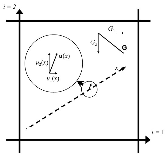
Figure 1.
2D rendering of a CV (thick solid lines), the associated ODT domain (dashed line), and their respective coordinate systems. The coordinates of the fixed Cartesian mesh of cubic CVs are labeled i, while x denotes the coordinate aligned with the ODT domain. The domain orientation is parallel to the time-varying domain-average velocity , which defines the corresponding unit vector . The components of the ODT vector property profile are , where and 2 in this 2D illustration. The pressure gradient has components where is the unit vector aligned with coordinate i. is more intuitively (though unconventionally) denoted in Equation (1) and elsewhere. For simplicity, a coarse-grained spatial discretization is assumed such that is uniform in the CV and therefore uniform in x in Equation (1).
The ODT state is subject to two advancement processes. One is viscous advancement governed by
In the last term, is density and is the index-i directional derivative of the LES-prescribed pressure, deemed to be spatially uniform within the ODT domain. In the other terms, derivatives after a comma are denoted t for time or x for spatial location on the ODT domain. This spatial treatent is not equivalent to the 1D projection of the Laplacian of the velocity vector onto the domain direction, which cannot be evaluated in ODT owing to its reduced dimensionality. Rather, viscous transport of the vector velocity is modeled as the viscous transport of the velocity components treated as three scalar fields, which qualitatively represents the vector process.
The other advancement process is a stochastic sequence of instantaneous eddy events that punctuate the viscous advancement. Each eddy event modifies the system state within some interval of the ODT domain coordinate x, so the subsequent resumption of viscous advancement starts from the new system state. For present purposes, no-flux conditions are applied at the domain endpoints.
An eddy event consists of two operations. One is a rearrangement of all property profiles within the eddy interval, termed the triplet map. It is defined on the 1D continuum coordinate x (see Section 6.1), but it is intuitive to interpret it as the continuum limit of a permutation of the cells of a uniform discretization of the x coordinate, where all cell properties are carried with the cell upon its displacement. (This is one, but not the only or preferred, numerical implementation of the map.) Within ODT, this map is a Lagrangian model analog of the advection operation of the Eulerian momentum equation.
In addition to advective and viscous transport, momentum advancement includes momentum sources and sinks, at a minimum the pressure-gradient field that enforces continuity in the flow regime of present interest. In the present formulation, these are introduced in two ways. For the case of laminar flow, hence no eddies, the model reduces to viscous transport and the LES-prescribed pressure gradient as shown in Equation (1). From the ODT perspective, that term is an external source (or sink) of momentum and kinetic energy. The eddies that introduce turbulence effects imply concomitant ODT-level pressure fluctuations. The ODT eddy representation of the effects of these fluctuations is self-contained the simplest situations, so their modeled effects should not change the domain-integrated momentum or kinetic energy. A representation of pressure fluctuations that obeys this constraint is introduced as an additional eddy operation after implementation of a triplet map. It is formulated concisely in terms of chosen functions that are added to the respective velocity components .
Momentum conservation must be obeyed by each individual velocity component but kinetic-energy conservation applies only to the sum of component kinetic energies. For the constant-density regime under consideration, these constraints require and . Other physically desirable properties are that is continuous and is nonzero only within the eddy range , where the latter reflects the association of the pressure fluctuation with the eddy motion. Additionally, requiring to be piecewise linear has proven to be mathematically convenient.
On this basis, the formulation is adopted, where is the map-induced displacement of the location x that is mapped to , here expressed as the inverse-map function . For constant density, this conserves momentum by construction while kinetic-energy conservation imposes one constraint on the coefficients .
Anticipating extension of this formulation to regimes such as variable-density flow, an additional function is introduced. Then the complete eddy event is the transformation
Here, it is convenient to represent the mapped component profiles as new functions of the fixed coordinate x rather than as the original functions with transformed arguments, so they are denoted . The coefficients and are chosen so as to change component momenta and kinetic energies subject to applicable conservation laws and additonal physical modeling sufficient to specify all the coefficient values uniquely. The evaluation of and on this basis is explained in Section 6.1 and Section 6.2.
The main physical content of ODT is the stochastic process by which eddy intervals and times of occurrence are determined. The profiles of the velocity components within the various possible eddy intervals are the inputs to that determination, and the kernels play a key role in the specification of the eddy rate distribution based on that input. has units time length such that is the rate of occurrence of eddies, whose left boundaries are within the range and whose lengths are within the range , where the argument t reflects the dependence of on the system state within at time t. The specification of and the way that it is used to sample eddy events are described in Section 6.3.
Although the profiles influence ODT advection by eddy events, they are not velocities operationally in the sense of appearing in a operator. Nevertheless, the statistical properties of these profiles are the principal model outputs, and it is important for these properties to faithfully represent the statistics of the physical flow field both for prediction purposes and in order for the SGS closure described here to be internally consistent. These requirements guide the formulation of ODT and its SGS implementation.
For given initial conditions, boundary conditions, and body forcings, if any, an ensemble of simulated realizations can be generated by running multiple realizations using a different random number seed for each. In this sense, ODT simulations are used to approximate the statistics of the ensemble, where the precision of the approximation depends on the number of realizations or, for statistically stationary flows, on the duration of the realization if a single realization is simulated. This raises the question of whether a formal mathematical representation of the underlying ensemble can be constructed. Such a construction is possible but has not previously been reported, so it is presented in Appendix A.
2.2. Coupling of ODT Domains
2.2.1. Lagrangian Formulation
ODT, as described in Section 2.1, differs from autonomous standalone ODT in that it includes the LES-prescribed pressure. This is one of the two types of large-scale input needed for SGS closure. The other required input is the set of LES face-normal velocities for all CVs, which are used to couple ODT domains in adjacent CVs.
This coupling is performed using a Lagrangian method that preserves the fine-scale flow features that are resolved within ODT. The approach is illustrated by comparing it to conventional Eulerian advective coupling of LES CVs involving a finite-volume treatment that does not resolve sub-structure within individual CVs.
For this purpose, consider constant-density finite-volume advection of a passive scalar field in 1D using a uniform mesh with cell width W. Continuity requires that all face velocities are identical, where the coordinate index is omitted for this 1D illustration. The discretized scalar field has scalar value in cell j. For the purpose of streaming the scalar along the 1D domain with velocity , treat the scalar s as a function of the continuum coordinate x. Because s is uniform within each cell, it is piecewise constant in x. Streaming for a time interval produces a shifted scalar profile . Box filtering within each cell gives, after rearrangement, , which is the lowest-order discrete upwind approximation of the Eulerian 1D advection equation
Although the spatial-continuum picture reduces to an Eulerian numerical algorithm, physically it prescribes Lagrangian time advancement as follows:
- Interpret the length-W portion of within each cell j as a separate length-W 1D domain denoted .
- For each j, remove an interval from the downstream end of and attach it to the upstream end of .
- Box filter each domain .
One consequence of the error inherent in the numerical approximation is that s is subject to numerical dissipation that is asymptotically diffusive over a long time interval with numerical diffusivity of order . The specific cause of this dissipation is the final box-filtering step. This step is omitted when using the procedure to couple adjacent ODT domains because the intent is then to preserve rather than suppress fine-scale structure. ODT advancement processes dissipate fluctuations induced by this coupling in a manner that models the physical processes governing dissipation, so dissipation in ODT is not a numerical artifact. Nevertheless, the Lagrangian coupling introduces property discontinuities that can be partially or totally mitigated depending on the flow regime, as explained shortly.
2.2.2. Domain Coupling in the Linear-Eddy Model
Although not yet implemented numerically for ODT SGS closure, this domain-coupling procedure is commonly used for SGS closure involving the linear-eddy model (LEM), which is the antecedent of ODT. Velocity profiles are not defined or time advanced in LEM. LEM evolves scalar fields on a 1D domain using a parameterized prescription of the statistics of eddy-event sampling (where an LEM eddy event is solely a triplet map) rather than a self-contained procedure. It is used as an SGS mixing and combustion closure for LES. Features common to the LEM and ODT SGS formulations are explained here in terms of LEM, omitting details documented elsewhere [1,2] that are not relevant here. As in LEM SGS implementation, the domain-coupling procedure described in Section 2.2.1 is termed splicing.
Each exemplar object receives inflow from the upstream side, which switches from one cell boundary to the other if the sign of is reversed. In contrast, each LEM domain has permanently assigned inflow and outflow ends, where the inflow is always received from the whatever direction is upstream at a given instant and the outflow is always directed in the current downstream direction. In a 3D LES CV, the LEM domain is analogous to a weather vane, whose center is fixed at the center of the LES CV. All inflows through the CV faces are appended to the tail while the current contents of the LEM domain are shifted commensurately toward the head. Outflows are produced by removing fluid intervals at the head of the domain and transferring one interval through each of the faces that, based on the sign of its face-normal velocity, is an outflow face. This process is illustrated in Figure 2.
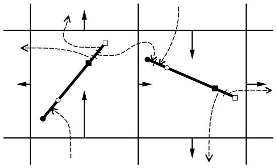
Figure 2.
Illustration of splicing-induced transfers of LEM domain segments to adjacent LEM domains. Solid lines with arrows are face-normal velocities that govern these transfers. Each 1D domain has an input end (circle) and an output end (square). Open and filled symbols demarcate the LEM domains before and after splicing. Segments transferred during splicing are separated by tick marks. Dashed curves with arrows indicate transfers between LEM domains in different CVs.
The LEM state associated with an LES CV is intended to be statistically representative of the physically correct population of SGS chemical compositions within the CV so that it provides accurate chemical closure information. For this purpose, LEM time advancement should capture the effects of all eddy motions not resolved at LES scales. This includes eddy motions as large as the size W of the CV, corresponding to eddy events of that size, so the LEM domain length D should be at least that large. This point is discussed further with reference to ODT in Section 7.1.
Another constraint is that the typical residence time of an LEM fluid parcel within an LEM domain should be roughly , which is the LES-prescribed flow-through time of the associated CV. This is desired because processes such as finite-rate chemistry within a CV imply a dependence of the chemical state of fluid exiting the CV on its residence time. More broadly, consistency between the SGS and LES advancement requires the SGS fluid parcels to follow trajectories through the flow domain that are consistent with the tracer statistics implied by the LES-resolved time advancement. Residence-time consistency is one facet of this requirement.
This ostensibly imposes the requirement , but as shown in Section 7, an additional degree of freedom is available to enforce the LEM residence time while allowing if the latter is desired, e.g., in order to reduce the statistical sample variability of outputs extracted from the LEM state.
2.2.3. Extension to ODT
The original ODT formulation [3] time advanced only one velocity component, denoted here as u. Although the SGS formulation requires the vector ODT formulation [4,5], some aspects of splicing are explained first with reference to a scalar velocity u for clarity. For this purpose, the configuration used to describe the application of splicing to the scalar field s is adopted, with u replacing s. Then on some ODT domain, whose x coordinate ranges, say, from 0 to W, splicing inserts some u profile into an interval , while now contains the u profile that previously occupied the interval . Owing to time advancement on all ODT domains prior to splicing, the profile after splicing is in general discontinuous at .
This discontinuity is an artifact of splicing that needs to be removed because the u profile governs eddy-event sampling (Section 2.1), and in particular generates an unphysical burst of small eddy events in the vicinity of a discontinuity. Two ways of removing the discontinuity are compared.
One approach is to box filter discontinuous velocity profiles. This conserves momentum but dissipates kinetic energy, with no kinetic energy remaining to be dissipated after that, as indicated by the fact that the kinetic-energy dissipation rate is then zero. This is analogous to the lowest-order ’production equals dissipation’ level of turbulence modeling, or it alternatively can be seen as analogous to implicit LES (ILES), in which the numerical algorithm provides the closure [6].
The other approach is to use the K and J kernels (see Section 2.1) to remove the discontinuity in a globally conservative manner. First, the piecewise constant function in , in is added to , where is set equal to the u discontinuity at so as to remove the discontinuity, and the condition enforces momentum conservation. This gives and . This adjustment causes some kinetic-energy change . It is counteracted to render the scheme conservative by adding to , where K is a kernel that is applied in this instance to and c is adjusted so that it causes the energy change . (As explained in Section 6.1, this involves solving a quadratic equation for c, where one of the two solution branches is identified as the physical solution. The discriminant can be negative, in which case energy conservation cannot be enforced, so some violations must be allowed.) The definition of implies , so the kernel addition does not change the total momentum on the ODT domain. For variable-density flow, both the K and J kernels are needed, involving an additional coefficient b (see Section 6.1), to enforce conservation as well as remove the discontinuity.
A CV in a 3D Cartesian mesh is subject to one splicing operation through each of its six faces during each time-advancement cycle. Then on average there are three segments appended to the inflow end of the associated ODT domain. The required adjustments can be implemented sequentially using the method described above after each attachment, or more efficiently with a slightly more complicated algebraic system that implements one adjustment accounting for all of the newly appended segments.
To sharpen the comparison of approaches, consider the special case in which the u profile on each ODT domain is initially spatially uniform, where the spatially uniform value is different on different ODT domains, indexed by j. This is analogous to the initial condition of the example. Then splicing induces ODT-level kinetic-energy nonuniformities, implying production of subgrid-scale turbulent kinetic energy (TKE). As noted, the first approach dissipates the TKE immediately. However, the adjustment after ODT splicing is globally (within each ODT domain) conservative and therefore is operationally an advective-transport mechanism rather than a dissipative process. This is consistent with the foundational principle that the effects of viscous and any other molecular transport processes on the ODT-level system states are implemented only through time advancement of molecular-transport equations, in the present instance Equation (1).
The practical consequence is that TKE dissipation in the ODT domains is the outcome of eddy-induced cascading of velocity fluctuations to the viscous scales, leading to viscous dissipation of those fluctuations. The resulting time lag from TKE production to transport, strain-induced scale reduction, and finally dissipation of TKE results in local imbalances between production and dissipation. Thus, these imbalances arise in a manner that is more closely linked to the governing physics than is the treatment provided by, e.g., a parameterized SGS kinetic-energy equation.
Advected scalars such as species mass fractions are not amenable to adjustments that remove scalar discontinuities owing to the stricter conservation laws that must be enforced locally in order to assure chemical realizability. Therefore, scalar discontinuities, including density discontinuities, are inherent artifacts of subgrid LEM and ODT formulations that involve splicing. They can be mitigated somewhat by coarsening the CVs, which reduces the splicing frequency. Because LEM and ODT fully resolve SGS turbulent cascading within the modeling framework, the desired fidelity might be achievable with coarser meshes than are usually used.
Numerical implementation considerations such as mesh resolution are similarly consequential with regard to algorithmic accuracy and stability. In past applications of LEM SGS closure of LES, benchmark tests of the splicing algorithm, such as rigid-body translation of a cylinder at some inclination relative to the Cartesian coordinates, have been conducted albeit not reported in publications. Mesh refinement studies demonstrated satisfactory convergence to the continuum limit, but for the mesh and time-step settings of practical computations, there was considerable dispersion and distortion. As indicated by the 1D analysis in Section 2.2.1, splicing is effectively first order in space and time with no available higher-order extension, so there is no obvious way to mitigate these numerical errors. In practice, this requires limitation of the application of splicing-based closure to cases for which these numerical effects are dominated by turbulent fluctuations. As shown, e.g., in [2], this encompasses a variety of regimes of interest.
Application of splicing to ODT domains is subject to these considerations as well as additional factors. First, in AME the CV face velocities that specify the volume fluxes governing the splicing operation are based on ODT flow states, as described next in Section 2.3. This introduces stochastic variations of those fluxes in space and time, which could promote numerical instability. Second, in CVs adjacent to walls, one endpoint of the associated ODT domain is attached to the wall. Splicing into or out of that endpoint could degrade the ODT representation of the near-wall flow. Strategies that avoid this, and accordingly differ from the procedure illustrated in Figure 2, are described in Section 4.
Overall, splicing is a necessary but imperfect mechanism for preserving the physical distinction between nondissipative advection and dissipative viscous and molecular-mixing processes. However, there are limited but significant applications for which purely Lagrangian LEM or ODT closure that eschews splicing is suitable. One such application is SGS mixing within the unresolved thickness of a time-varying internal fluid interface such as a flame front, a case in which the LEM domain orientation is locally normal to the front rather than locally aligned with the flow [7].
2.3. Time-Advancement Cycle
As in Section 2.2, the notional time-advancement cycle for a simple ILES analog is outlined to serve as a reference point for description of the low-Mach-number time-advancement cycle for ODT-based SGS closure:
- Within each CV, labeled by index j, the spatially uniform velocity is subject to pressure forcing that adds to , where the components of are the quantities in Equation (1) and is the cycle time step.
- The next step is a pressure projection using the CV velocities as input. Based on a staggered scheme, this yields updated CV pressures and CV face-normal velocities that are in conformance with the continuity equation.
- The updated face-normal velocities are interpolated to update the quantities .
- Advection of the velocities as prescribed by the CV face-normal velocities is implemented as a 3D generalization of the discretized advection of the scalar in Section 2.2.
The numerical diffusivity associated with the advection operation, noted below Equation (3), is not necessarily an accurate representation of SGS advective transport, which is why the algorithm is termed an ILES analog rather than an ILES. In any case, this sequence of operations is LES-like advancement of the momentum equation although it is not a conventional LES procedure.
The analogous time-advancement cycle for ODT-based SGS closure is as follows:
- Based on Equation (1) or some generalization of it such as in Section 5, each ODT domain is time advanced for an elapsed time . This involves sub-cycling over smaller time intervals owing to the smaller CFL time for the well-resolved ODT mesh. This advancement is subject to interruptions to implement eddy events. No-flux boundary conditions are applied at the ODT domain endpoints unless a wall boundary condition is applied at one of the endpoints. The ODT wall treatment is explained in Section 4.
- For each ODT domain, the average velocity vector is evaluated by box filtering the ODT flow state. The resulting filtered flow field is interpolated to evaluate the face-normal velocities , which are the inputs to a pressure projection that enforces consistency of the face-normal velocities with the spatially discretized continuity equation, as required for consistent implementation of splicing. The momentum interpolation in conventional pressure projection schemes [8,9] needs modification owing to the nonstandard AME procedures for momentum advancement (eddy events and splicing).
- For each CV, the quantity in Equation (1) now has a new value based on the updated CV pressures that is denoted . Accordingly, the fixed pressure-gradient value that should have been used during the time advancement of the associated ODT domain is the interpolant . If the ODT domain is not wall-bounded, then is modified for consistency with advancement during based on rather than by adding , uniformly over x, to the profile . If the ODT domain is wall-bounded, this would violate the no-slip boundary condition at the wall, reflecting a splitting error resulting from not applying the pressure-gradient forcing in Equation (1) on a fully synchronous basis. For this case, an approach that was shown to work well in [10] is applied. Namely, instead of incrementing uniformly over x, the correction is added to . This yields a consistent value and obeys the no-slip condition at the wall location .
- Splicing is applied as in Section 2.2.3.
A key feature of the approach is that steps 2–4 fulfill the requirements for coarse-grained advancement of the momentum equation, complementing the fine-grained advancement during step 1. Splicing requires coarse-grained information that is ultimately provided by the pressure projection, which is a correction that enforces a constraint rather than a time-stepping procedure. The correction involves the use of an auxiliary equation that is structurally a coarse-grained momentum equation but is not time advanced, as explained Appendix B.
On this basis, it is fair to say that this formulation involves no time advancement of a filtered momentum equation. In that sensem the formulation is an outgrowth of prior efforts to construct a bottom-up multiscale turbulence simulation based on ODT, notably the approach termed ODTLES [11,12,13]. The present approach is structured more like LES/LEM than like ODTLES, which involves direction-dependent hybridization of resolved and coarse-grained momentum advancement. Because the new feature is the avoidance of any time advancement of a filtered momentum equation, the approach is termed autonomous microstructure evolution (AME). This feature does not assure consistently advantageous cost/performance outcomes relative to ODTLES or conventional LES. Future studies will identify the classes of problems for which the respective approaches are advantageous.
As in ODTLES, AME distinguishes between velocity profiles that represent the flow states on the ODT domains and velocities that govern coarse-grained advection. The latter are in this respect auxiliary variables. The coarse-grained flow state represented by the set of velocities is likewise auxiliary from the ODT perspective, but from the coarse-grained perspective, the velocities constitute the desired flow solution. In LES implemented on a staggered mesh, the distinction between and is purely algorithmic, while in AME there is a further distinction because is a coarse-grained approximation of the detailed physical representation of the evolving flow state produced by ODT. A nuance in this regard is that there is a fine-grained representation of the advection induced in AME by the velocities , as explained in Section 3.
Finally, it is noteworthy that the velocities are adjusted to satisfy the 3D continuity equation but no such requirement is imposed on the ODT velocity profiles . Unlike , these are not advecting velocities although they influence the sampling of eddies that implement 1D advection on the ODT domain. Eddy advection is performed by triplet maps that obey the 1D analog of continuity by construction - namely, the total arc length of the mapped interval(s) is the same after a triplet map as before.
3. Reynolds Stress and Subgrid-Scale Kinetic Energy
The analogy between AME and LES that is described in Section 2.3 applies to physical interpretation as well as numerical modeling of time-advancement processes, particularly with regard to the SGS TKE budget. Features of SGS TKE production, transport, and dissipation in the ODT SGS closure are discussed conceptually in Section 2.2.3. They are now considered with reference to the formal definitions of these quantities in LES.
SGS TKE production is more precisely described as the conversion of coarse-grained kinetic energy into SGS TKE. One factor in the expression for the conversion rate is the Reynolds stress, whose evaluation in AME is considered first.
Splicing is the AME implementation of coarse-grained advection. Splicing is CV-to-CV transfer of portions of ODT velocity-component profiles, generically denoted u, where the transfer is governed by CV face velocities, generically . (Vector operations and the associated component indexing conform to standard conventions so scalar notation is used for clarity.) The u fluctuation profile on an ODT domain is denoted . The SGS TKE (per unit mass in what follows) is generically denoted , ignoring both component indexing and summation over components. Consistent with this, a 1D array of CVs is considered (or equivalently, a multidimensional array with nonzero spatially uniform in only one direction), as in Section 2.2.1.
On an ODT domain , suppose that a sub-interval is designated to be transferred to the ODT domain in the CV to its right, corresponding to positive . In a coarse-grained sense, the displacement of this sub-interval is , while the remainder of the u profile is unmoved by this transfer in a coarse-grained sense. (As explained in Section 7, D can exceed W while nevertheless representing the flow state in the width-W extent of the CV in direction x. Here, the default case is chosen for simplicity.) On this basis, the coarse-grained displacement of the u profile is zero except for the selected size- interval. The advecting velocity governing the displacement of that interval is denoted . Accordingly, the profile of the advecting velocity in is
Box filtering of v over the ODT domain gives and hence . This identifies the ODT profile of the velocity fluctuation as
This shows that the face velocity can be interpreted as a box-filtered velocity, thus motivating the notation that has been adopted.
Similarly, the fluctuation of the advected velocity is . Spatial averaging of the product of and then gives the contribution of the outbound transfer of the size- interval to the box-filtered Reynolds stress,
where denotes the average of u over and is the outflow endpoint D of the ODT domain.
The outbound fluid is replaced by inbound fluid occupying a size- interval for which owing to its attachment to the inflow endpoint. The ODT state in the CV that supplies this fluid is denoted . The filtered value of the interval that is transferred rightward, denoted , is in general different from , where the notation refers to the distinct size- intervals containing the inbound and outbound fluid respectively. The inbound and outbound transfers convert the original profile u into a new profile U. Box filtering of U gives , where denotes the average of u over the size region not removed during the outbound transfer.
The inbound fluid enters the CV through the face opposite to the outflow considered thus far. As noted, has the same value at both faces, which is reflected by the equal sizes of the advected fluid intervals. The box-filtered Reynolds stress associated with the inbound transfer is
where is specified by Equation (5) with u replaced by .
The new total (filtered plus SGS) kinetic energy is , which is the sum of the filtered and SGS kinetic energies, and respectively, where . Similarly, the initial SGS kinetic energy is , where . Then the splicing-induced SGS TKE change is expressed as
consisting of conversion of filtered kinetic energy into SGS kinetic energy, advection by the resolved flow, turbulent transport , subgrid transport , and viscous dissipation , respectively.
This specializes the conventional decomposition of [14] to the setup analyzed here. The conventional pressure and viscous transport terms are omitted because splicing involves no represention of SGS pressure fluctuations or viscous fluxes across cell faces. is included to indicate that dissipation of SGS TKE occurs during ODT advancement, as explained in Section 2.2.3. Because the splicing operation is not dissipative, is omitted from the application of Equation (8) to splicing that follows.
The approach is to evaluate using the appropriate specializations of the terms on the right-hand size and then to compare the outcome to the conventional expression for and . Extending interval-restricted averaging to arbitrary powers p of u and , the identities
and
will be useful in what follows. As before, each size- averaging interval begins at the lower boundary of the removed or inserted interval and refers to the complement of that interval on the ODT domain.
Evaluation of using Equations (9) and (10) gives
In accordance with the relation , this change is attributed to the time-advancement step . For simplicity, Equation (11) is specialized to vanishing , so . Noting that converges to in this limit, the leading-order result
is obtained.
In the conventional decomposition of , and in the present reduced notation. In Equation (8), a difference of values separated in time by is analyzed, so the conventional terms are multiplied by , which will lead to cancellation of based on . Additionally, each spatial derivative is replaced by times a difference between the CV in which the is analyzed and the CV to its left, whose velocity profile has been denoted . Finally D is changed to W owing to the specialization to .
On this basis,
and
are obtained, giving
In Equation (8), with omitted, substitution of results for the terms that have been evaluated gives
Rewriting this as
each term is the product of a discretized derivative of filtered u velocity and a flux-type factor involving only filtered fields. This result is compared to the conventional expressions and , where the spatial discretization reflects the evaluation of the Reynolds stresses as domain averages rather than point values at domain endpoints. This gives . Using Equations (6) and (7) to evaluate the Reynolds stresses,
is obtained.
Equation (17) reproduces the discretized derivative terms in Equation (18). To fully reproduce Equation (18), must be replaced by where appears in each of the terms multiplying a discretized derivative. This is equivalent to adding to each of these occurrences of . In the limit of vanishing W, cell-to-cell variation becomes asymptotically small such that is asymptotically small relative to , hence negligible. This shows that the difference between Equations (17) and (18) an order-of-accuracy discretization effect rather than a difference in the physics that is represented, thereby demontrating the physical correspondence between the subgrid stress associated with splicing and the subgrid stress inferred from the conventional LES formalism.
The term in Equation (16) is of divergence form (first difference of a function of a filtered quantity), identifying it as the subgrid transport term . Hence, the remaider of Equation (16) corresponds to the conversion term . This completes the evaluation of the terms of the budget.
The use of closure models that resolve the processes governing evolution eliminates the need for modeled equations for that are otherwise used for closure in various LES formulations [14]. Within the AME framework, the evaluation of budget terms is for diagnostic purposes rather than for LES closure and serves to highlight the correspondence to the conventional LES formalism. Additionally, budget diagnosis of AME simulation results potentially can aid in the formulation of modeled SGS equations for conventional LES, which are often elaborate, involving multiple equations [14]. This is an example of the potential use of AME to improve more economical LES formulations.
Moreover, the formal analysis of Reynolds stresses is directly involved in AME numerical implementation. In Appendix B, the Reynolds stresses given by Equations (6) and (7) are needed inputs to the evaluation of eddy viscosities in the equation solved by the pressure projection.
4. Extension to Wall-Bounded Flow
The formulation thus far addresses bulk-flow closure. Wall boundary layers require special treatment, in accordance with previous ODT near-wall treatments. Previous applications of ODT to wall boundary layers include multiphysics cases [15,16,17], and ODT has been implemented as a near-wall SGS closure in LES of channel flow [10,18]. That formulation is potentially suitable for near-wall closure within the present framework, but it involves under-resolved time advancement, so in keeping with AME concept, an alternative procedure is outlined.
A CV in a cuboidal flow domain has as many as three faces that are adjacent to walls. Such a CV is assigned as many ODT domains as the number of such faces, where each domain is associated with one of those faces and is deemed to be normal to that face. The domains associated with a given CV are treated as independent during ODT time advancement. As in [10], each domain is attached at one of its endpoints to its associated face and ODT advancement within the domain is subject to the boundary condition at that endpoint, while a no-flux boundary condition is applied at the other endpoint.
Consider splicing for the case in which each CV involved in this operation has one face adjacent to a wall. Each of the associated ODT domains has only one free endpoint available for splicing, so this becomes both the inflow and outflow point. All assigned outflows emanate sequentially from that endpoint, after which all assigned inflows are attached sequentially at that endpoint.
A limitation of this procedure is that there is no direct flow from the innermost sub-layer in a wall-bounded ODT domain to its downstream neighbor. However, there is an indirect communication path, as follows. Wall-normal turbulent transport in the ODT domain associated with the upstream CV can advect near-wall fluid close enough to the outflow endpoint of the ODT domain so that it can be spliced to the ODT domain in the downstream CV, followed by wall-normal turbulent transport down to the near-wall region of that ODT domain. Owing to the slowness of near-wall flow, this is the dominant mechanism of streamwise transport of near-wall fluid over large streamwise distances, but not necessarily between adjacent CVs. These assertions are supported by quasi-steady-quasi-homogeneous theory and its validations [19], which indicate that small-scale near-wall motions (resolved by ODT in AME) depend primarily on the larger-scale local flow state (controlled by splicing in AME).
In contrast, the method in [10,18] includes Eulerian implementation of direct advective transport, at each height above the wall, between parallel ODT domains in neighboring wall CVs. This is under-resolved time advancement of advection, hence outside the scope of the AME concept, but its adoption could be advantageous, depending on the application.
The treatment of CVs for which faces are adjacent to the wall is based on the interpretation of the f associated ODT domains as f instances of the representative state within the CV. Then the average over all f domains is deemed to be the average state of the CV, e.g., for the purpose of evaluating . Likewise the adjustment based on the pressure projection is applied to all f domains, so the individual domains will have different filtered velocities.
For splicing in a block-cuboidal domain with cubic meshing, the possible pairs of f values in the donor and receiver CVs are , , , , , , , , , and . Tetrahedral edge and corner CVs in an unstructured mesh allow the additional possibilities , , , , , and but exclude some of the cubic-mesh pairings. Further, for , splicing involving a pair of ODT domains within a given CV is possible. Specification of physically consistent splicing protocols for the various cases is straightforward but tedious and will be addressed as such cases arise in future applications.
5. Extension to Variable Density
5.1. Boussinesq Approximation
The model description thus far has been restricted to constant-property flow in order to introduce the approach in the simplest possible context. The first step in the extension of the scope of the model is its generalization to variable density, which is considered next.
The minimal dynamical effect of density is obtained in the Boussinesq approximation, in which density is held fixed at a reference value except in a gravitational forcing term proportional to the small local deviation of the density from the reference value. In ODT, the representation of this forcing depends on the ODT domain orientation.
On a horizontal domain, the forcing is applied during viscous advancement by adding the gravitational forcing term to Equation (1) for the velocity component that is vertically oriented. Then relabeling the density in Equation (1) as to indicate that it is a spatially uniform reference density, the gravitational forcing is added to the equation for the vertical velocity component, nominally the equation. Owing to spatial variation of the density profile , time advancement of the modified equation tends to produce velocity fluctuations along the ODT domain, thereby contributing to eddy occurrences as governed by the sampling procedure described in Section 6.3. Variants of this approach have been applied to buoyancy-driven boundary layers along vertical walls [16,20,21].
On a vertical domain, a triplet map applied to a domain interval in which varies will in general change the eddy-integrated gravitational potential energy. The energy change is an input to the kernel procedure, which imposes an equal-and-opposite change of the eddy-integrated kinetic energy of the velocity profiles (see Section 6.1) and consequently influences the sampling of eddy occurrences (see Section 6.3). Details of this approach evolved in a series of publications [3,15,22,23,24,25,26,27].
Reflecting the inflow-outflow treatment of non-wall ODT domains, each of them is deemed to be aligned with the current orientation of its time-varying filtered velocity . Accordingly, the gravity vector is decomposed into components perpendicular and parallel to . The effect of the perpendicular (parallel) component is then represented as it would be on a horizontal (vertical) ODT domain. In this way, the formulation reduces to the implementations for the respective special cases.
Because and therefore its orientation vary during ODT advancement, the domain orientation should ideally be re-evaluated continually for accurate treatment of the gravitational forcing. Since the variation of orientation is caused primarily by filtered-scale processes (splicing and pressure correction), it is nevertheless sufficient to re-evaluate it once per time-advancement cycle in keeping with splitting errors inherent in the multiscale formulation. (From this viewpoint, the pressure forcing in Equation (1) can likewise be applied only once per time-advancement cycle with negligible overall loss of fidelity.)
For conservative tracking of gravitational potential energy changes, the ODT domain must be fully specified with reference to the fixed coordinate system. A natural convention is to locate the domain midpoint at the CV center (suitably defined for CVs in an unstructured mesh). Then an orientation change corresponds to a rotation with respect to the domain midpoint. Unless the axis of the rotation is vertical, this implies vertical displacements of fluid elements. Provided that this motion is implemented once per time-advancement cycle and specifically in conjunction with splicing, the associated change of gravitational potential energy can be compensated by a change of kinetic energy that contributes to the overall kinetic-energy change during the kernel operation associated with the removal of splicing-induced discontinuties of velocity profiles, as described in Section 2.2.3.
This mechanism can likewise subsume gravitational-potential-energy effects associated with all fluid displacements that occur during splicing, including fluid shifts along the ODT domain resulting from outbound and inbound fluid transfers at opposite ends of the domain. There is splitting and spatial-discretization error associated with the displacements that occur during this operation, but it is again within the scope of error that is inherently associated with the coarse-grained evolution.
A principal application of Boussinesq buoyant stratified flow is geophysical flow. For this application, ODT SGS resolution can extend the scale range of the simulation relative to conventional LES, but not to the finest scales of turbulent motion. In this context, ODT needs closure at its resolution scale. Standalone ODT with such a closure has been used for simulation of the atmospheric boundary layer [15,28]. ODT and LEM have also been used as SGS scale-range extensions for the purpose of moist-thermodynamics closure in LES of clouds [29,30], albeit with a different strategies for coupling ODT and LEM to LES than proposed here.
5.2. Density Variation without Dilatation
The full variable-density treatment in AME, with buoyancy effects omitted, is described next. If density is a spatially nonuniform advected quantity on the ODT domain with no density changes in the Lagrangian frame, then the density profile evolves within ODT solely by triplet mapping. (An example of this regime to which ODT has been applied is immiscible fluids advected by turbulence [31].) Density nonuniformity is nevertheless dynamically consequential in ODT because it influences eddy-event occurrences and the coefficients of the kernels that are applied during eddy events, as explained in Section 6. Further, Equation (1) is generalized to the variable-density form
where is the dynamic viscosity.
These effects ultimately modify the CV face velocities and hence splicing as well as the outcome of pressure projection. The influence is two-fold. First, the evolution of the ODT velocity profiles is modified as indicated. Second, box filtering on the ODT domain now requires Favre (mass-weighted) averaging to obtain the mass-averaged velocities needed at the coarse-grained level.
This raises the point that coarse-grained mass-averaged velocities are based on box filtering over ODT domains, but domain intervals that are spliced across CV faces generally have different average densities than the ODT domains from which they are taken. Therefore, ODT cannot precisely match the mass fluxes implied by the box-filtered density and velocity fields. This is a feature rather than a deficiency, reflecting ODT-resolved property fluctuations, whose effects are not captured at the coarse-grained level. In any case, fluid transfers across CV faces are most consistently specified on a volumetric basis (see Section 7.1), so the mass-flux mismatch is immaterial to the implementation of splicing.
The effect of the pressure forcing in Equation (19) on momentum is spatially uniform, but with density variation this implies a source of velocity fluctuations that can contribute to the available energy that induces eddy events, as explained in Section 6. This is the ODT representation of baroclinic vorticity generation. Standalone ODT can at best (and only for compressible flow [32]) incorporate pressure gradients aligned with the domain, so baroclinic vorticity can be represented only in SGS ODT coupled to advancement of the coarse-grained pressure field.
The projection of the pressure forcing in the ODT domain direction implies a bulk acceleration of the domain that can alternatively be diagnosed from the time evolution of . This acceleration is analogous to gravitational forcing. In variable-density flow it induces the Rayleigh–Taylor instability, to which ODT has been applied [27]. Thus, standalone ODT captures the instability based on prescribed gravitation or acceleration and SGS ODT can represent it as a response to the coarse-grained acceleration field.
A related mechanism involving the effect of body forces in variable-density flow is the Darrieus–Landau instability. It is specifically associated with dilatational effects, as discussed in Section 5.3 and Section 6.3, and is represented in standalone as well as SGS ODT implementation.
Unlike the ODT velocity profiles, density profiles cannot be adjusted after splicing to remove discontinuities, so these discontinuities persist and potentially adversely impact model fidelity with respect to both the eddy-event time history, as explained in Section 6, and the advancement of Equation (19). It will be important to assess the effects of this artifact on model performance. Some considerations in this regard, including possible mitigation strategies, are discussed in Section 7.1 and Section 8.
5.3. Dilatational Flow
If additionally there are Lagrangian density changes, then there is a commensurate dilatational flow along the 1D domain because it is treated as a closed system during ODT advancement. Then Equation (19) is generalized to
Here, a dilatational velocity profile is introduced that is based on 1D continuity in Lagrangian form, giving , where the material derivative is determined by the physical processes driving the dilatation, e.g., thermal expansion. This determines to within an arbitrary constant, implying the freedom to advect the 1D domain by any uniform velocity. In Equation (20), advects the ODT momentum profiles , which are advected scalars from an operational viewpoint at the ODT level. Additionally, appears in a source term at the end of Equation (20) that is explained in what follows.
Dilatation changes the length of the ODT domain. As noted in Section 2.2, the model is consistent for any domain length equal to or larger than the CV scale. The handling of variable-length ODT domains during the time-advancement cycle is discussed in Section 7.1.
Recognizing that varies with time as well as with ODT domain location x, the dynamical implications at both the ODT-resolved and coarse-grained levels are considered. Bulk translation of the entire ODT domain is governed by CV face velocities that prescribe the splicing of fluid between ODT domains. The variable-density ODT-level processes that influence this coarse-grained transport have been noted in the discussion of dilatation-free variable-density ODT in Section 5.2. The net outcome is that global changes of the total momentum of the ODT domain are captured in Equation (20) by the pressure-gradient forcing, as prescribed by the pressure projection. Therefore, the undetermined constant in the evaluation of is assigned by requiring the implied domain-integrated momentum change to be zero. This avoids any double-counting of effects captured by coarse-grained processes during the time-advancement cycle.
In the chosen frame, the spatial variation of dilatation can drive or suppress momentum fluctuations and is a source of kinetic energy that is generated by the mechanism driving the dilatation, such as exothermic chemical reactions. These consequences of dilatation are incorporated into ODT by the source term in Equation (20). This expression projects , which is vectorially aligned with the ODT domain-orientation unit vector , onto the unit vector that is aligned with the coordinate direction i (see Figure 1).
As a special case, assume that the viscous and pressure terms in Equation (20) are zero, that the ODT domain is aligned with the coordinate , and that and initially. For any subsequent time history of the profile, Equation (20) then implies that , as required.
Because the components do not advect fluid along the ODT domain, there is a decoupling of the momentum and kinetic-energy changes such that the latter will not precisely reflect the conversion from thermal to kinetic energy that is induced by the dilatation. The overall self-consistency maintained by the time-advancement cycle suggests that the energy conversion process will be roughly conservative, but this remains to be demonstrated. An analogous treatment of dilatation in an application of standalone ODT to turbulent combustion [33] yielded accurate results.
Local accelerations associated with transient fluctuations of , in conjunction with the density variations that drive them, induce the Darrieus–Landau instability. This instability mechanism is incorporated into ODT as a contribution to the frequency of eddy occurrence, as explained in Section 6.3.
6. The ODT Eddy Event
6.1. Eddy Implementation
Some details of ODT eddy implementation are explained. Except where new or modified features are introduced, physical justification and interpretation are minimal because they are provided in the cited references.
An ODT eddy event involves two operations. The first is a mapping denoted and termed the triplet map that is applied to a selected (see Section 6.3) interval . Within this interval, every property profile s is subject to three-fold compression and the mapped interval is filled with three copies of the compressed profile, but the middle copy is spatially flipped. Outside this interval, is unchanged.
Each is mapped to three locations . It is sometimes convenient to refer to the single-valued inverse map for given and l. Denoting the mapped property profile as , this gives . Based on this meaning of , the generic argument x, and hence the notation , is used in what follows.
On a fixed uniform 1D mesh, the triplet map is approximated using a permutation of mesh cells [1]. An alternative approach that has proven to be advantageous is to use an adaptive mesh that allows implementation of the continuum definition of the triplet map as well as the continuum mathematical specfication of splicing procedures. Adaptive-mesh ODT implementation, as described in [21], is assumed here in all explanations of ODT and AME.
The second operation, which is applied only to velocity components, is the kernel addition shown in Equation (2). This operation is the model representation of scale-l pressure-fluctuation effects, reflecting the pressure-gradient term in the momentum equation. In this regard, the pressure-gradient term in Equation (1) is the filtered pressure computed during the pressure-projection step. No explicit model of ODT-resolved pressure fluctuations per se has been formulated for low-Mach-number flow.
The K and J kernels induce pointwise velocity changes and domain-integrated kinetic-energy changes. Additionally, J (always) and K (in variable-density flows) individually induce domain-integrated momentum changes, sometimes with equal and opposite effects so as to obtain zero net change. For a given velocity component, these changes can involve kinetic-energy exchange with other components as well as with momentum and kinetic-energy sources and sinks associated with coupling to processes involving, e.g., gravitational potential energy, surface-tension energy, or entrained particles or droplets. In Section 2.2.3, kernels are used to restore energy conservation after piecewise-uniform adjustments of velocity profiles to remove discontinuities.
These kernel effects and the applicable conservation laws constrain the coefficients and in Equation (2) as follows. For variable-density flow, momentum conservation implies
Integration over reflects the volume interpretation of the ODT domain based on the cross-sectional area introduced in Section 7.1. The integrals extend over the entire domain, but the integrands are zero outside the eddy interval so they can be equivalently restricted to that x range. The argument x is henceforth omitted. Here and below, a previous constant-density treatment [34] that introduced momentum and energy sources (or sinks) and respectively is extended to variable-density flow by bringing into all integrands. This results in minor generalizations of the algebraic solutions in [34]. Details that are readily inferred from that treatment are omitted here.
Because the triplet map conserves total momentum, can be substituted for in the integrand on the right-hand side. This cancels a term on the left-hand side, reducing Equation (21) to
This relation can be substituted for in equations that follow, reducing them to relations for the unknowns . The solution for then determines using Equation (22). Because , Equation (22) directly evaluates if is spatially uniform.
The eddy-induced change of the domain-integrated kinetic energy of velocity component i is
Conservation of total kinetic energy by the triplet map allows to be substituted for in the second integral, resulting in a cancellation of terms that gives
Substitution of Equation (22) for yields a quadratic equation for , whose solution straightforwardly generalizes Equation (11) of [34].
is thus specified in terms of and functionals of the flow state. Energy conservation imposes the constraint , leaving two additional degrees of freedom governing the allotment of this net kinetic-energy change to the three components.
For this purpose, additional modeling is introduced. Although a constant-density treatment for any combination of momentum and energy sources [34] and a variable-density treatment involving only energy sources [5] are available, there is no prior variable-density treatment involving both types of sources. This is needed for the use of kernels in Section 2.2.3 to correct conservation violations caused by flow-field adjustments to remove splicing-induced discontinuities. Equation (24), in conjunction with the energy-allocation scheme introduced in Section 6.2 to specify the required energy changes , provides the needed model extension.
Given the quantities and and the flow state, Equations (22) and (24) can be solved for . It is possible for the discriminant of the solution to be zero or negative, corresponding to an energetically prohibited event. For this and other reasons (see Section 6.3), a sampled eddy event is not necessarily implemented.
If the discriminant is positive, then the quadratic equation has two real solutions. The solution branch is chosen on the basis of the functional dependence of on . As monotonically approaches zero starting from its assigned value, one of the solution branches approaches , corresponding to no change of the flow state in the absence of a required energy change. The solution based on the assigned value that corresponds to this branch is deemed to be the physically consistent solution.
6.2. Allocation of Kinetic-Energy Changes
Rotational eddy motion can redistribute kinetic energy among velocity components. Existing formulations of the kernel operation, such as in [34], take this into account. Depending on the application, the net kinetic-energy change might be specified on a component-wise basis, hence for each component i, but the rotational eddy motion similarly justifies modification of this allocation. (To preserve momentum conservation in ODT, which is a vector constraint on each individual momentum component, momentum is not redistributed among components.)
To narrow the range of options, it is noted first that there is a state-dependent bound on the amount of kinetic energy that can be extracted from a velocity component using kernels. It is determined by minimizing with respect to using Equation (24). The absolute value of this negative quantity is termed the component-i available energy . The variable-density expression for is a straightforward generalization of Equation (12) of [34]. Through the dependence of Equation (24) on , depends on the momentum sources .
The total available energy of the post-map velocity field is then and the net available energy, accounting also for energy sources, is . If , then is an energy sink requiring a greater reduction in kinetic energy than the maximum possible reduction Q, so the eddy is deemed to be forbidden. (Criteria for eddy occurrences are explained in Section 6.3.) Therefore, nothing further needs to be said about this case, so what follows is restricted to .
The simplest assumption is that the final eddy state has no memory of details of the initial state or external sources, so H is the sole governing quantity on which to base the enforcement of energy conservation. Then the final component-i available energies are because there is no basis for different outcomes for different components.
This is a good baseline model and perhaps the only needed model. It implies the component-i available-energy change , where subscripts j and k refer to the coordinate indices not equal to i. If , this is the usual energy redistribution for , where denotes the coefficient of .
To extend this minimal formulation, a physical basis is needed for arriving at unequal values of the final component available energies . The initial component available energies are the physically compelling basis for this because component energies are properties of the ODT physical state, involving no additional external input. This consideration, in conjunction with (1) the physical principle that an eddy region cannot supply more energy to an external sink than the eddy region contains, and (2) the additional straightforward, though not physically required, assumption that the dependence of on is linear, yields the generalized formulation
where is a ‘memory’ parameter. This recovers for the ‘no-memory’ value . Because and H are non-negative and , is also non-negative provided that . The definition of available energy precludes negative , so a value of outside this range could yield a mathematical inconsistency.
The definition of as originally stated [4] does not uniquely specify the treatment of energy sources. For , and are linearly related according to , where the range corresponds to the range . Then the equivalent result is obtained, which has the advantage that it uses the existing notational convention, but at the cost of less clarity with regard to the assumptions that extend the treatment to nonzero sources. However, the notation does clarify one point. is the fraction of the component-i available energy that is transferred, in equal shares, to the other two components by the kernels, which requires its range to be . This explains the less intuitive range of the parameter .
Regardless of the number and types of physical processes contributing to , this input suffices in this formulation to determine the quantities and H and thus the energy changes that are used to calculate the coefficients . On this basis, a wide range of physical processes and their couplings interact with eddy implementation (and sampling - see Section 6.3) within a unitary framework.
For spatially uniform and no energy or momentum sources, substitution of Equation (22) into Equation (24) indicates that the terms involving cancel. Then the integrand reduces to , which is non-negative. As expected for a state with zero kinetic energy, kernels can increase but not decrease the total kinetic energy, indicating that the component-i available energy is zero. Eddy selection, as described in Section 6.3, is based on available kinetic energy. In particular, positive available kinetic energy is required in a selected interval in order for an eddy to be implemented in that interval. Therefore, if all velocity components are uniform within the eddy range and there are no external sources, the eddy event is not implemented. Accordingly, the available-energy formalism satisfies the requirement that density variation in the absence of velocity fluctuations or an external source cannot induce eddy events. In buoyant stratified flow, the gravitational-potential-energy change resulting from triplet mapping a gravitationally unstable density profile is an external source that can generate eddy events in initially motionless fluid. This is the basis of ODT applications to buoyancy-driven flow that are discussed in Section 5.1.
6.3. Eddy Sampling
The physical reasoning and formal analysis on which eddy sampling is based are discussed in detail in references cited below. Here, the concepts are briefly outlined and the mathematical expression for the eddy rate distribution that is derived in those references is presented and explained.
As in mixing-length theory, is expressed dimensionally in terms of the relevant length scale, in this case l, and a modeled time scale , giving . Unlike conventional mixing-length theory, the value of l is specific to each event rather than a fixed function of spatial location, and depends on the instantaneous system state in the size-l eddy interval rather than mean values of bulk metrics of the flow.
The model adopted for [35], re-expressed in present notation, is
where
- , , and is the eddy volume.
- is the net final available energy, now interpreted as the kinetic energy associated with the eddy motion.
- , where and are the -averaged dynamic viscosity and density, respectively. ( is a harmonic average.) is a viscous penalty that suppresses eddies that are subject to sufficient viscous damping to prevent their occurrence. (A negative argument of the square root indicates that the eddy has insufficient net final available energy to overcome viscous suppression.)
- C and Z are adjustable model parameters.
- The term is the underlying dimensional estimate of . Other quantities in Equation (26) are based on a variable-density formulation [5] that consistently generalizes an earlier constant-density expression for , including equivalent definitions of model parameters.
With the choice in Equation (25), corresponding to the value used almost all ODT studies to date, eddy implementation is effectively parameter-free and thus universal. Thus, all case-dependent behavior is embodied in the rate distribution from which eddies are sampled. This is reflected in order-one variation of the best-fit parameter values for different classes of flows.
For unconfined flows that impose no intrinsic limitation on the largest eddy size , various empirical principles have been invoked to suppress unphysically large eddies [5]. In SGS implementation of ODT, C and have been set by requiring the mesh-resolved and ODT SGS energy spectra to be complementary in wave-number range, without a gap or overlap, and to satisfy an amplitude matching condition at wave number [11]. These are internal consistency requirements, involving no empirical input, so the only empirically tuned parameter is Z, which is tuned to match the empirical dissipative roll-off of the energy spectrum. (For wall-bounded ODT domains, Z is chosen to match the transition from the viscous layer to the buffer layer [10].) In AME, will be of order W, so self-consistent determination of C and can be performed using domain sizes that allow the possibility of . The implications of with regard to splicing are discussed in Section 7.1.
constrained by the assigned size bound fully determines the statistics of eddy occurrences. Efficient sampling from this time-evolving distribution is needed for cost-effective numerical implementation. Because depends only on the current system state with no explicit dependence on past history, eddy occurrences constitute a Poisson process in time. The thinning method, in which a Poisson event process is oversampled but events are selectively rejected so as to recover the correct sampling statistics, can therefore be used for eddy sampling. Details of the application of this method to sampling from are provided in the Appendix of [21].
The central role of the net available energy in both the selection and implementation of eddy events has been highlighted. The scope of the phenomenology that this approach can capture is illustrated by ODT modeling of the Darrieus–Landau instability in premixed flames. Local accelerations induced by thermal expansion are equivalent to body forces that can result in the equivalent of triplet-map-induced changes of gravitational potential energy in variable-density flow, as explained in Section 5.3. This equivalent gravitational effect, represented in ODT as an external source contributing to the available energy so as to increase the amplitudes of the applied kernels, thereby promoting eddy occurrences, has been incorporated into combustion simulations as a representation of the Darrieus–Landau instability [16,33]. SGS ODT in AME can similarly capture this phenomenology.
7. Details of the Splicing Procedure
7.1. Enforcement of Consistent Volume Transfers
In this section, it is convenient to refer to ODT SGS closure of LES, but references to LES likewise apply to the coarse-grained fields in AME. The unclosed LES property fields that SGS ODT is intended to close are intensive properties. For this purpose, each ODT domain serves as a representative sample of flow states that can be averaged in order to obtain closure in the associated CV. This allows freedom to set the ODT domain length so that ODT provides a sufficient statistical sample of flow states for closure purposes, subject to other requirements. The relevant considerations are examined with reference to a cubic LES mesh and then generalized to an arbitrary unstructured mesh.
During an advancement step corresponding to a time increment , the volume transfer across an LES CV face is , where is the face-normal velocity and is the face area. In order to accommodate such LES-level transfers on a consistent volumetric basis, each ODT domain is assigned a nominal volume that is equal to the volume V of the associated CV, where D is the domain length and is a nominal cross-sectional area, hence . To accommodate the LES-prescribed rate of volume inflow on the ODT domain, the nominal splicing-induced flow velocity along the ODT domain must be . The corresponding residence time of fluid on the ODT domain is .
For the example in Section 2.2.1, the fluid residence time in a CV is . The cubic-mesh relations and reduce the ODT residence-time result to the same expression, showing that the proposed volumetric interpretation of the ODT domain is consistent in this regard.
Expressing this another way, the LES face velocity implies a displacement of a fluid element of length across the face in time , but for , the corresponding length of the spliced ODT interval is . Although the volumetric picture involving and is useful for motivating this splicing-length rule, numerical implementation requires only the application of this rule. In this regard, serves no purpose other than helping to motivate this rule and therefore has no physical significance nor does it have any role in model implementation.
As noted, may be desired based on sample-size considerations. Sample-size requirements related to the ODT representation of backscatter are discussed in Section 7.3. An ODT SGS closure of LES of clouds provided indications that produced insufficient sampling [30]. That formulation did not involve splicing, but was found to be sufficient in a cloud LES study using LEM SGS closure with splicing [29]. Both formulations involved dynamically active feedback of SGS moist thermodynamics to LES-resolved scales. ODTLES applications without such feedback did not indicate sample-size insufficiency, but the numerically dissipative domain coupling in ODTLES could have contributed to the suppression of fluctuations. These disparate observations do not point to any firm conclusions other than to say that the sample-size requirement might depend on both the application case and details of the model formulation.
Another consideration with regard to the domain size is that ODT eddy events should span a size range such that the combination of splicing and ODT eddy events captures the full spectral range of turbulent eddy motions, with neither double-counting nor gaps, as explained in Section 6.3. For a different form of ODT SGS closure, it was found that eddy events extending to size were required for this purpose [11]. This is qualitatively reasonable because the typical displacement of a fluid element by a triplet map is less than half the map size.
For variable-density and other variable-property flows, another advantage of is that it allows a significant interval of the domain starting from the inlet endpoint to be omitted from both filtering and the gathering of output data. This would reduce the impact of splicing-induced property discontinuities introduced near the inlet on the overall flow evolution. (Molecular transport mollifies these discontinuities before they are advected far from their points of origination.) For velocity profiles, the procedure for removing discontinuities is stated in Section 2.2.3 to involve kernels applied to the interval , but more generally they should be applied to , which includes the case assumed in that discussion.
Irrespective of the presence or absence of splicing-induced discontinuities, there is another potential artifact near both the inlet and outlet endpoints of the ODT domain. The no-flux boundary conditions applied at those endpoints (see Section 2.1) result in suppression of eddy-induced transport that might have occurred near those locations if the domain were instead unbounded, in effect creating a numerical boundary layer at each endpoint. Each occurrence of splicing refreshes these peripheral zones so the artifact might not be consequential. If it is nevertheless significant in some cases, then omitting regions near both endpoints from filtering and data gathering could be beneficial, subject to consideration of any conservation violations that might result from this.
In the general case of an unstructured mesh, CVs might have different volumes V and CV faces might have different areas , so the volumetric picture is generalized accordingly. Subject to the considerations that have been noted, any choices of the domain lengths D of individual ODT domains based on user-specified criteria are allowed, so in general these domains will have different nominal cross-sections . Consider a volume transfer from CV 1 to CV 2 across a face of cross-section , corresponding to a face-normal fluid-element displacement . This implies splicing of an ODT interval of length out of CV 1, but volume preservation implies that it arrives in CV 2 with length . Thus for , the length of the spliced interval must be rescaled by the factor in order to preserve volume.
Because this rescaling is a volume-preserving change of the shape of the spliced interval, the resulting stretching or shrinking of the length of individual fluid elements does not imply any density changes. This rescaling modifies the length scales of flow structures represented by ODT property profiles, and hence is a model artifact. Provided that is neither very large nor very small, the artifact is not necessarily severe because it is akin to the physically based triplet-map-induced rescalings of intervals of the ODT domain. It can be avoided by assigning a fixed ratio , hence fixed , to all CVs, but this might not be the optimal choice based on other considerations.
For dilatational flows the situation requires further explanation because the D value changes during the ODT advancement within each time-advancement cycle. This is a operator-splitting effect resulting from the fact that fluid-element density changes are accommodated during ODT advancement by varying the domain length. This is rectified during the pressure-projection step, which assigns CV face velocities so as to produce a net volume transfer into or out of a CV that is equal and opposite to the net volume change implied by the ODT advancement. The indicated adjustments involving the possibly CV-specific and values remain valid, here assuming that splicing restores the D value corresponding to the CV volume.
If ODT were used as an SGS closure of unclosed terms in an LES rather than within the AME framework, then the LES advancement might produce CV face velocities that do not precisely restore the prior D values of all ODT domains. This can be rectified by rescaling ODT domain lengths as needed to enforce the desired domain lengths and then using the relation to update . The adjustment should be small if there is reasonable consistency between ODT and LES advancement.
7.2. Ordering of Fluid Transfers
During each time-advancement cycle, a segment of an ODT domain is transferred across each CV face. For a CV with f faces, this involves some number of inbound transfers and outbound transfers. (For non-dilatational flow, i cannot be 0 or f because these values would imply a change of the CV volume.) Figure 2 illustrates a portion of a notional 2D flow domain with Cartesian meshing and hence , with on the left side and on the right side.
For , the order in which inbound segments are attached to the ODT domain must specified. As in [36], residence-time considerations are invoked to address this. Suppose , corresponding to two inbound segments, whose volumes are denoted and , with . If segment 2 is attached first, followed by segment 1, then segment 2 is immediately positioned a relatively substantial fraction of the distance from the inflow to the outflow endpoint of the domain, shortening its residence time prior to its eventual expulsion of its contents. Although the choice of ordering does not affect the mean residence time of fluid in the CV, the ordering 2 followed by 1 will tend to broaden the residence-time distribution relative to the choice 1 followed by 2. In the absence of evidence to the contrary, the default procedure should be to keep the residence-time distribution as narrow as possible. Accordingly, the attachments should be performed in decreasing order of segment volumes.
Now consider two outbound transfers requiring volumes . Based on the same consideration, in what order should they be implemented? Detaching a segment of volume first would enable the second transfer to occur from a region relatively close to the inflow endpoint, corresponding to a relatively short residence time of the transferred segment. Therefore, the default ordering for outbound transfers is from smallest to largest segment volumes, where this choice is subject to comparison of the resulting residence-time distribution to any available empirical evidence.
7.3. SGS Contribution to Face Velocities
As noted in Section 3, conventional LES closures involve some implicit or explicit modeling of . This enables estimation of a subgrid velocity fluctuation that has been used to model backscatter by adding random increments of this order of magnitude to the filtered face velocities [14].
This raises the conceptual question of whether ODT SGS closure requires some analog of this additional procedure in order to model backscatter. This question has physical implications with regard to the choice of the ODT domain size, which affects the statistical variability of filtered quantities as noted in Section 7.1. In the limit of infinite ODT domain size, filtered ODT property profiles converge to ensemble-average values of the filtered properties. Then in this limit, the filtered properties have the same meaning as in conventional LES, so as in LES, additional modeling would be needed in order to capture backscatter. The choice of a finite ODT domain size, which is a practical necessity, introduces finite-sample variability that can be viewed as either an error source relative to conventional LES or as a supplement to conventional LES in that it provides a model representation of backscatter as an inherent attribute of ODT.
Like any other model feature, the validity and fidelity of this backscatter representation depends on the physical realism of ODT flow advancement, but it also requires an objective basis for choosing the ODT domain size so as to obtain the physically correct degree of finite-sample variability. Backscatter modeling in conventional LES provides guidance in this regard. Because is a diagnosed property of the ODT state, can be evaluated. Then the ODT analog of conventional backscatter modeling is obtained when the domain size is chosen so that the finite-sample variability of values obtained for given flow conditions is of order as determined from the ODT results. Relatively large ODT domains might be needed for multiphysics cases, e.g., with reaction-driven thermal expansion, owing to the intensity and sporadic occurrences of the associated backscatter effects. Based on the identified self-consistent choice of domain size, the resulting finite-sample variability of would be imprinted on the face velocities by the pressure projection. (This happens whether or not the procedure is optimized as described.)
In Section 2.3, the importance of generating realistic fluid-parcel trajectories through the flow domain was noted. This depends upon both the evaluation of the CV face velocities and the splicing protocol. For a splicing-based LEM closure of LES that lacked the SGS flow information provided by ODT, a particle-tracking approach involving an autocorrelated stochastic velocity contribution modeled SGS fluctuation effects on the splicing-induced fluid-parcel trajectories [29]. This improved the model representation of turbulent dispersion. With ODT closure, it is possible that fluctuations induced by ODT statistical variability will adequately capture this effect.
8. Discussion
LEM and ODT have been used in various ways for SGS closure of LES, such as for chemistry closure of reacting flow simulations, for near-wall momentum closure, and in ODTLES, which involves direction-dependent hybridization of resolved and coarse-grained momentum advancement. The present formulation is based on the viewpoint, within the low-Mach-number framework, that a broad range of turbulence phenomenology and associated microphysics can be well represented by modeling momentum advancement on a fully resolved basis, using only the coarse-grained pressure-projection step to capture global effects. The absence of time stepping of coarse-grained momentum or scalar transport equations motivates the description of the approach as autonomous microstructure evolution (AME).
As in LEM chemistry closures, one ODT domain is associated with each coarse-grained control volume. Relative to that and other previous formulations, AME includes the following novel features:
- The distribution of the available kinetic energy among velocity components during the kernel operation is consistently formulated for the general case of arbitrary external energy and momentum sources and sinks.
- Alignment of the orientation of each ODT domain with the evolving coarse-grained flow is enforced. Nevertheless, velocity components are defined in the fixed coordinate system of the physical domain.
- As in LEM SGS closure, the splicing operation that implements fluid transfers between ODT domains is governed by the coarse-grained velocity field but the transferred parcels maintain full spatial resolution of property profiles. A novel feature is the subsequent adjustment of velocity profiles that eliminates splicing-induced discontinuities subject to the applicable conservation constraints.
- A volumetric interpretation of splicing-induced fluid transfer provides flexibility with regard to the choice of ODT domain lengths while maintaining physically consistent fluid residence times on the ODT domains, and it straightforwardly generalizes to an unstructured mesh.
- A fine-grained interpretation of the splicing operation enables a physically consistent formulation of the Reynolds shear stress, enabling a prescription for diagnosing the terms of the SGS turbulent-kinetic-energy budget.
- The freedom to assign the ODT domain length, in combination with the availability of SGS TKE statistics, offers the possibility of a self-consistent quantitative approach to the representation of backscatter.
- A splicing protocol specialized to ODT domains attached to a wall at one endpoint incorporates the dominant fluid-transfer mechanism in boundary layers.
- For variable-density flow, the projection of the coarse-grained pressure gradient onto the ODT domain orientation identifies the bulk acceleration of the domain. On this basis, the Rayleigh–Taylor instability mechanism is embedded in the eddy selection and implementation procedures.
- For buoyant stratified flow in the Boussinesq approximation, a synthesis of standalone ODT formulations for horizontal and vertical domains respectively yields a formulation that is applicable for arbitrary domain orientation.
These features and the framework that encompasses them, embodied in the time-advancement cycle outlined in Section 2.3, offer the prospect of improved cost-performance characteristics relative to conventional LES and existing LEM and ODT closure formulations. This will be elaborated in sequels to the present contribution.
The adjustment of velocity profiles to eliminate splicing-induced discontinuities avoids a potential artifact, but it has been noted that this remedy is not applicable to density and other advected scalar fields. The alternative remedy of using long domains and excluding a limited neighborhood of the inlet endpoint from filtering operations applied to these property fields has been proposed. In this regard, several points are relevant. First, this artifact does not arise in constant-density flow or in buoyant stratified flow in the Boussinesq approximation, allowing a wide scope of AME application that is not subject to this artifact. Second, LEM SGS closure of mixing and chemical reactions in LES is subject to this artifact, yet its performance is satisfactory for a variety of combustion applications [2].
Finally there is the mitigation strategy of coarsening the mesh. Regardless of the ODT domain sizes in individual CVs, for a given mesh a fluid element must pass through the same number of CVs in order to traverse the flow and hence is spliced that number of times. A reduction in the number of splicings can only be achieved by coarsening the mesh.
This raises the question of the mesh resolution requirement in AME. AME time advancement is structured to involve only minimal large-scale influence through the pressure-projection operation, where the justification is that ODT is formulated to adequately represent flow phenomenology at all scales below those dominated by case-specific 3D large-scale forcings and constraints such as inflows, outflows, and boundary conditions. Therefore, a coarse very-large-eddy-simulation (VLES) type of mesh is not only viable but is central to the AME concept. The efficacy of coarse meshing has been shown in applications of ODTLES [11,12].
Coarse meshing not only mitigates any splicing artifacts but also reduces computational cost. For a flow that would require DNS CVs, AME with CVs where would require order fully resolved cells per ODT domain for a total of ODT cells. Assuming that computation time scales with the total number of ODT cells, this corresponds to a cost-reduction factor relative to DNS. This cost reduction could somewhat or entirely compensate for the cost of ODT relative to other SGS closures, depending on the case. Experience with ODTLES has indicated that the parallel-processing efficiency of SGS ODT results in acceptable turnaround times on high-performance computers [13].
Apart from the discontinuity artifact, splicing is a numerical form of ‘mesomixing’ (meaning at subgrid scale, but not at the molecular-mixing microscale) in the same sense that the ODT eddy event is a physically based mesomixing operation. This aspect of splicing is analogous to numerical dissipation in LES that can dominate the physical based dissipation if it is not carefully managed. Mesh coarsening reduces the number of times that a fluid element is spliced as it traverses the flow but the number of physical mesomixing events during the traversal, whether modeled as eddy events or resolved on the 3D mesh, is unchanged. Thus, mesh coarsening has the additional advantaged of reducing numerical mesomixing relative to physically based mesomixing, thus enhancing the physical fidelity of the numerical implementation.
High fidelity with VLES-type meshing is plausible for simple flows such as the canonical free-shear flows. In the near-wall regions of boundary layers and confined flows, the demonstrated performance of ODT as a standalone and an SGS near-wall model [10,11,12,16,18,21] provides assurance that the ODT near-wall formulation for AME described in Section 4 will likewise provide suitable closure on a coarse mesh.
Unsteady boundary layers are subject to local flow separation and re-attachment. Related features such as recirculation zones arise in bulk flow. The compatibility of the present formulation with unstructured meshes provides the flexibility to refine the mesh adaptively so as to increase spatial resolution when and where it is needed. Where the local refinement leaves an insufficient range of subgrid scales to benefit from the multiscale ODT treatment, the splicing protocol can be retained but box filtering can be applied after each splicing operation so as to implement the no-model closure described in Section 2.2.1.
An approach to adaptive meshing termed the arbitrary Lagrangian Eulerian (ALE) method [37] employs operator splitting consisting of Lagrangian implementation of advection and Eulerian implementation of molecular transport. The mesh adaption advects CV faces, involving no property fluxes across faces. This overcomes the advective CFL time-step limitation although there remains a weaker time-step bound that prevents topologically forbidden mesh structures and related anomalies. After mesh adaption, the flow state is mapped onto an improved mesh structure, causing redistribution of fluid volumes among CVs. This implements the physically prescribed molecular-transport fluxes across CV faces.
In AME with ALE meshing, splicing is decomposed into two operations. First, the ODT domains are displaced in accordance with the advection of the CVs containing them. Second, the mesh remapping prescribes transfers of domain segments across CV faces. This implementation reduces both splicing frequency and volume fluxes per splicing occurrence, thus mitigating numerical artifacts as in conventional ALE.
SGS ODT within the AME framework has been emphasized because this is convenient for explaining the closure approach without reference to the particulars of LES implementation. Addressing SGS ODT within an LES framework in full detail requires consideration of the interactions between the numerical and physical modeling implementations in a particular LES code, which is beyond the present scope. Nevertheless it is pertinent to note that a basic requirement for closure of LES (and likewise AME, as shown in Appendix B) is evaluation of the filtered Reynolds stresses. In Section 3 a formalism for their evaluation based on analysis of the SGS TKE budget is developed and is shown to be broadly consistent with the Navier–Stokes equation-based LES formalism.
Another potential application of ODT SGS closure is motivated by LEM chemistry closure of LES [2]. The LES provides LEM with CV face velocities that govern splicing and a parametric representation of SGS turbulence that controls LEM SGS advection. The only LEM input to LES flow advancement is the filtered divergence, deduced from volume creation caused by thermal expansion, that is used to solve the coarse-grained pressure Poisson equation. ODT could be used in this formulation instead of LEM. ODT would receive additional input from the LES in the form of pressure-gradient forcing of the ODT momentum equation, but would provide the same output as LEM to the LES flow advancement. The ODT filtered flow field would then be at best roughly consistent with the LES flow field, but this should be sufficient for the intended chemistry closure. The potential benefit of the use of ODT instead of LEM is relaxation of the restriction to standard inertial-range similarity scalings, instead allowing dynamical effects such as SGS baroclinic vorticity, the Darrieus–Landau instability, and the kinematical effects of thermally induced viscosity fluctuations to be captured. Importantly, this substitution is not simply a matter of replacing LEM by ODT in existing formulations. As explained in Section 2.2.3, it also requires the application of a specialized splicing protocol to ODT velocity profiles.
The present restriction of AME to low-Mach-number flow is a consequence of the exclusion of coarse-grained momentum advancement. The relaxation of this restriction by extending the scope of ODT SGS implementation to LES closure leads to consideration of closure of compressible LES formulations using low-Mach-number ODT as described here or its extension to compressible flow [32]. In applications to supersonic inert mixing [38] and to detonation phenomena [39,40], LEM has been used for subgrid mixing/reaction closure in which high-speed effects are communicated by the LES thermodynamic inputs to LEM. This is a suitable strategy for some purposes, but ODT SGS closure, especially if compressible, would extend the scope of application of LES to high-speed flows. The dynamically based ODT representation of SGS kinetic energy (Section 3) would be a pertinent input to the LES energy equation.
Thus, the novel flow-advancement features that have been described have potential benefits beyond AME per se. Similarly, AME can be supplemented by coarse-grained advancement in particular situations in which it is advantageous, as illustrated by a previous approach to ODT-based near-wall closure that is mentioned in Section 4. Another example, noted in Section 5.1, is buoyant stratified flow at geophysical scales, for which SGS ODT can serve as a scale-range extension relative to conventional closures, but cannot affordably resolve the physical microscales and accordingly requires its own SGS closure. Although coarse-grained in this sense, this formulation preserves the defining AME feature that there is no time advancement of a momentum equation on the filtered 3D mesh.
Details of the numerical implementation of AME will be presented in a future publication, accompanied by applications to canonical flows for demonstration and validation purposes. The relative performance of alternative strategies for model formulation or numerical implementation that have been noted will be evaluated, involving tradeoffs with regard to physical soundness, numerical accuracy, and computational cost. For clarity of interpretation, the initial test cases will be simple and in some instances within the scope of the capabilities of conventional LES, ODTLES, or standalone ODT. These steps are targeted on the principal goal of capturing the configuration-specific coupled dynamics of microphysical processes and high-intensity turbulence that are difficult to investigate using presently available methods.
Funding
This research received no external funding.
Acknowledgments
The author thanks Jackson Mayo for contributing the analysis presented in Appendix A.
Conflicts of Interest
The author declares no conflict of interest.
Abbreviations
The following abbreviations are used in this manuscript:
| ALE | Arbitrary Lagrangian Eulerian |
| AME | Autonomous microscale evolution |
| CFL | Courant-Friedrichs-Lewy |
| CV | Control volume |
| DNS | Direct numerical simulation |
| ILES | Implicit large-eddy simulation |
| LEM | Linear-eddy model |
| LES | Large-eddy simulation |
| ODT | One-dimensional turbulence |
| Probability density function | |
| SGS | Subgrid-scale |
Appendix A. Functional Fokker–Planck Equation Governing the Time Evolution of the Probability Distribution of ODT Flow States
For constant-property ODT, the system configuration is denoted and is treated as a scalar (one-component) field; generalization of what follows to the vector velocity field is straightforward. Stochastic ODT evolution of u can be expressed in terms of the single-time PDF of all possible system configurations u. Its time advancement is governed by the functional Fokker–Planck equation
On the right-hand side, the first term represents Liouville evolution of the PDF due to the deterministic viscous advancement based on viscosity , where prime denotes x-derivative and a functional derivative is applied to the quantity in braces. The second term represents the loss in probability for the configuration u due to eddy events, which occur at the rate and lead to configurations different from u. The third term represents the gain in probability for the configuration u due to eddy events that lead to u from all other possible configurations , weighted by , the eddy rate , and the eddy parameter PDF , where denotes the parameters that specify a given eddy; the functional delta function restricts the functional integration over configurations to the relevant events, such that the post-eddy configuration equals u. LEM is the special case in which the rate and the PDF are independent of u. ODT/LEM numerical simulation can be viewed as a Monte Carlo method for solving this Fokker–Planck equation; other approximate solution methods may be available.
Appendix B. Pressure Projection in AME
Pressure projection is conventionally applied to the Navier–Stokes equation by taking the divergence of the equation and then invoking the continuity equation to obtain a Poisson equation that is solved to obtain an updated pressure field and then adjust the flow state so as to enforce continuity. In AME, the flow state that must obey continuity is the set of CV face velocities , while pressure values reside at CV centers.
The AME pressure projection is based on the synthetic 3D momentum equation
where is a spatially varying eddy viscosity that is evaluated as a Cartesian tensor using the gradient-transport relation
Here, the derivative of in direction j is evaluated as a first difference between the CVs that share the face that is crossed by the flux, while the contributions of splicing operations to the Reynold stresses are obtained using Equations (6) and (7). Based on the synthetic momentum equation with evaluated as indicated, the pressure Poisson equation is derived and solved computationally in discrete form. (A well-behaved numerical scheme has been formulated and will be described elsewhere.)
The synthetic 3D momentum equation is at best an approximation of the coarse-grained dynamics of the current flow state at the time of the pressure adjustment. As such, it introduces modeling error in the same sense that the idealized ODT flow representation introduces modeling error. Importantly though, it is an auxiliary equation that is re-initialized during each time-advancement cycle rather than evolving persistently in a manner that could become deoupled from, and therefore inconsistent with, ODT-level flow advancement.
Indeed, the pressure adjustment as a whole does not involve time advancement and the quantities are auxiliary variables, whose adjustment has no direct effect on any of the ODT property profiles, which constitute the flow state. In this sense, the pressure projection per se does not time advance the flow state although it does evaluate the pressure field, which is a physical output, albeit under-resolved.
References
- Kerstein, A.R. Linear-eddy modelling of turbulent transport. Part 6. Microstructure of diffusive scalar mixing fields. J. Fluid Mech. 1991, 231, 361–394. [Google Scholar] [CrossRef]
- Menon, S.; Kerstein, A.R. The linear eddy model. In Turbulent Combustion Modeling: Advances, New Trends, and Perspectives; Echekki, T., Mastorakos, E., Eds.; Springer: Berlin/Heidelberg, Germany, 2011; pp. 221–244. [Google Scholar]
- Kerstein, A.R. One-dimensional turbulence: Model formulation and application to homogeneous turbulence, shear flows, and buoyant stratified flows. J. Fluid Mech. 1999, 392, 277–334. [Google Scholar] [CrossRef]
- Kerstein, A.R.; Ashurst, W.T.; Wunsch, S.; Nilsen, V. One-dimensional turbulence: Vector formulation and application to free shear flows. J. Fluid Mech. 2001, 447, 85–109. [Google Scholar] [CrossRef]
- Ashurst, W.T.; Kerstein, A.R. One-dimensional turbulence: Variable-density formulation and application to mixing layers. Phys. Fluids 2005, 17, 025107, Erratum in Phys. Fluids 2009, 21, 119901. [Google Scholar] [CrossRef]
- Grinstein, F.F.; Margolin, L.G.; Rider, W.J. Implicit Large Eddy Simulation: Computing Turbulent Fluid Dynamics; Cambridge University Press: Cambridge, UK, 2007. [Google Scholar]
- Schmidt, H.; Klein, R. A generalized level-set/in-cell-reconstruction approach for accelerating turbulent premixed flames. Combust. Theor. Model. 2003, 7, 243–267. [Google Scholar] [CrossRef]
- Majumdar, S. Role of underrelaxation in momentum interpolation for calculation of flow with nonstaggered grids. Numer. Heat Transf. 1988, 13, 125–132. [Google Scholar] [CrossRef]
- Bartholomew, P.; Denner, F.; Hazmil Abdol-Azis, M.; Marquis, A.; van Wachem, B. Unified formulation of the momentum-weighted interpolation for collocated variable arrangements. J. Comput. Phys. 2018, 375, 177–208. [Google Scholar] [CrossRef]
- Schmidt, R.C.; Kerstein, A.R.; Wunsch, S.; Nilsen, V. Near-wall LES closure based on one-dimensional turbulence modeling. J. Comput. Phys. 2003, 186, 317–355. [Google Scholar] [CrossRef]
- Schmidt, R.C.; Kerstein, A.R.; McDermott, R. ODTLES: A multi-scale model for 3D turbulent flow based on one-dimensional turbulence modeling. Comput. Methods Appl. Mech. Eng. 2010, 199, 865–880. [Google Scholar] [CrossRef]
- Gonzalez-Juez, E.; Schmidt, R.C.; Kerstein, A.R. ODTLES simulations of wall-bounded flows. Phys. Fluids 2011, 23, 125102. [Google Scholar] [CrossRef]
- Glawe, C.; Medina, J.A.; Schmidt, H. IMEX based multi-scale time advancement in ODTLES. Z. Angew. Math. Mech. 2018, 98, 1907–1923. [Google Scholar] [CrossRef] [Green Version]
- Sagaut, P. Large Eddy Simulation for Incompressible Flows, 3rd ed.; Springer: Berlin/Heidelberg, Germany, 2006. [Google Scholar]
- Kerstein, A.R.; Wunsch, S. Simulation of a stably stratified atmospheric boundary layer using one-dimensional turbulence. Bound. Layer Meteorol. 2006, 118, 325–356. [Google Scholar] [CrossRef]
- Monson, E.I.; Lignell, D.O.; Werner, C.; Hintze, R.S.; Finney, M.A.; Jozefik, Z.; Kerstein, A.R. Simulation of ethylene wall fires using the spatially-evolving one-dimensional turbulence model. Fire Sci. Tech. 2016, 52, 167–196. [Google Scholar] [CrossRef]
- Klein, M.; Schmidt, H.; Lignell, D.O. Stochastic modeling of surface scalar-flux fluctuations in turbulent channel flow using one-dimensional turbulence. Int. J. Heat Fluid Flow 2022, 93, 108889. [Google Scholar] [CrossRef]
- Freire, L.S.; Chamecki, M. Large-Eddy Simulation of smooth and rough channel flows using a one-dimensional stochastic wall model. Comput. Fluids 2021, 230, 105135. [Google Scholar] [CrossRef]
- Chernyshenko, S. Extension of QSQH theory of scale interaction in near-wall turbulence to all velocity components. J. Fluid Mech. 2021, 916, A52. [Google Scholar] [CrossRef]
- Dreeben, T.D.; Kerstein, A.R. Simulation of vertical slot convection using one-dimensional turbulence. Int. J. Heat Mass Transf. 2000, 43, 3823–3834. [Google Scholar] [CrossRef]
- Lignell, D.O.; Kerstein, A.R.; Sun, G.; Monson, E.I. Mesh adaption for efficient multiscale implementation of One-Dimensional Turbulence. Theor. Comput. Fluid Dyn. 2013, 27, 273–295. [Google Scholar] [CrossRef]
- Wunsch, S.; Kerstein, A.R. A model for layer formation in stably stratified turbulence. Phys. Fluids 2001, 13, 702–712. [Google Scholar] [CrossRef]
- Wunsch, S.; Kerstein, A.R. A stochastic model for high Rayleigh-number convection. J. Fluid Mech. 2005, 528, 173–205. [Google Scholar] [CrossRef]
- Gonzalez-Juez, E.; Kerstein, A.R.; Lignell, D.O. Fluxes across double-diffusive interfaces: A one-dimensional-turbulence study. J. Fluid Mech. 2011, 677, 218–254. [Google Scholar] [CrossRef]
- Gonzalez-Juez, E.; Kerstein, A.R.; Shih, L.H. Vertical mixing in homogeneous sheared stratified turbulence: A one-dimensional-turbulence study. Phys. Fluids 2011, 23, 055106. [Google Scholar] [CrossRef]
- Schmidt, H.; Kerstein, A.R.; Wunsch, S.; Nédélec, R.; Sayler, B.J. Analysis and numerical simulation of a laboratory analog of radiatively induced cloud-top entrainment. Theor. Comput. Fluid Dyn. 2013, 27, 377–395. [Google Scholar] [CrossRef]
- Gonzalez-Juez, E.D.; Kerstein, A.R.; Lignell, D.O. Reactive Rayleigh-Taylor turbulent mixing: A one-dimensional-turbulence study. Geophys. Astrophys. Fluid Dyn. 2013, 107, 506–525. [Google Scholar] [CrossRef]
- Freire, L.S.; Chamecki, M. A one-dimensional stochastic model of turbulence within and above plant canopies. Ag. Forest Meteorol. 2018, 250–251, 9–23. [Google Scholar] [CrossRef]
- Hoffmann, F.; Yamaguchi, T.; Feingold, G. Inhomogeneous mixing in Lagrangian cloud models: Effects on the production of precipitation embryos. J. Atmos. Sci. 2019, 76, 113–133. [Google Scholar] [CrossRef]
- Stechmann, S.N. Multiscale eddy simulation for moist atmospheric convection: Preliminary investigation. J. Comput. Phys. 2014, 271, 99–117. [Google Scholar] [CrossRef]
- Movaghar, A.; Linne, M.; Herrmann, M.; Kerstein, A.R.; Oevermann, M. Modeling and numerical study of primary breakup under diesel conditions. Int. J. Multiphase Flow 2017, 98, 110–119. [Google Scholar] [CrossRef] [Green Version]
- Jozefik, Z.; Kerstein, A.R.; Schmidt, H. Simulation of shock-turbulence interaction in non-reactive flow and in turbulent deflagration and detonation regimes using one-dimensional turbulence. Combust. Flame 2016, 164, 53–67. [Google Scholar] [CrossRef]
- Jozefik, Z.; Kerstein, A.R.; Schmidt, H.; Lyra, S.; Kolla, H.; Chen, J.H. One-dimensional turbulence modeling of a turbulent counterflow flame with comparison to DNS. Combust. Flame 2015, 162, 2999–3015. [Google Scholar] [CrossRef] [Green Version]
- Fistler, M.; Lignell, D.O.; Kerstein, A.R.; Oevermann, M. Turbulence modulation in particle-laden, stationary homogeneous isotropic turbulence using one-dimensional turbulence. Phys. Rev. Fluids 2020, 5, 044308. [Google Scholar] [CrossRef]
- Lignell, D.O.; Lansinger, V.B.; Medina, J.; Klein, M.; Kerstein, A.R.; Schmidt, H.; Fistler, M.; Oevermann, M. One-dimensional turbulence modeling for cylindrical and spherical flows: Model formulation and application. Theor. Comput. Fluid Dyn. 2018, 32, 495–520. [Google Scholar] [CrossRef]
- Arshad, S.; Kong, B.; Kerstein, A.R.; Oevermann, M. A strategy for large-scale scalar advection in large eddy simulations that use the linear eddy sub-grid mixing model. Int. J. Numer. Methods Heat Fluid Flow 2018, 28, 2463–2479. [Google Scholar] [CrossRef]
- Donea, J.; Huerta, A.; Ponthot, J.-P.; Rodrıguez-Ferran, M. Arbitrary Lagrangian–Eulerian methods. In The Encyclopedia of Computational Mechanics; Wiley: Hoboken, NJ, USA, 2004; Volume 1, pp. 413–437. [Google Scholar]
- Sankaran, V.; Menon, S. LES of scalar mixing in supersonic mixing layers. Proc. Combust. Inst. 2005, 30, 2835–2842. [Google Scholar] [CrossRef]
- Maxwell, B.; Pekalski, A.; Radulescu, M. Modelling of the transition of a turbulent shock-flame complex to detonation using the linear eddy model. Combust. Flame 2018, 192, 340–357. [Google Scholar] [CrossRef]
- Maxwell, B.M.; Bhattacharjee, R.R.; Lau-Chapdelaine, S.S.M.; Falle, S.A.E.G.; Sharpe, G.J.; Radulescu, M.I. Influence of turbulent fluctuations on detonation propagation. J. Fluid Mech. 2017, 818, 646–696. [Google Scholar] [CrossRef] [Green Version]


Publisher’s Note: MDPI stays neutral with regard to jurisdictional claims in published maps and institutional affiliations. |
© 2022 by the author. Licensee MDPI, Basel, Switzerland. This article is an open access article distributed under the terms and conditions of the Creative Commons Attribution (CC BY) license (https://creativecommons.org/licenses/by/4.0/).