Abstract
Flow mapping around bridge piers is crucial in estimating scour development potential under different flow conditions. The reliable measurement of turbulence and the estimation of Reynolds stress can be achieved on scaled models under controlled laboratory experiments using high-frequency Acoustic Doppler Velocimeter Profilers (ADVP) for flow measurement. The aim of this paper was to obtain operation parameters for an array of Vectrino Profilers for turbulent flow field measurement to reliably measure the flow field around bridge piers. Laboratory experiments were conducted on a scaled river model set up in an open channel hydraulic flume. Flow field data were measured on three characteristic profiles, each containing five measurement points collected by ADVPs configured as an array of two instruments. The determination of the operation parameters was done as a two-step process—calibration through the flume’s pump flow rate and verification with Acoustic Doppler Current Profiler RioGrande field data. Based on the results, the following setup for ADVPs’ operation parameters can be used to obtain reliable flow data in the scour hole next to the bridge pier: adaptive Ping Algorithm, Transmit Pulse Size of 4 mm and Cell Size of 1 mm.
1. Introduction
Insight into the flow environment in rivers across different scales and timeframes is important for all applications relying on detailed flow intensity information, such as the conveyance capacity of vegetated channels [1], environmental impact assessment for energy harvesting structures such as hydrokinetic turbines [2] or tidal turbines [3], the quantification of biogeochemical fluxes [4], suspended-sediment transport [5] or the morphodynamic evolution of confluences [6], to name a few. Environmental flows are challenging to observe and map due to the complex interaction of channel and overbank flow [7], flow in the river bends [8] and confluences [9]. Flow field data measurement is commonly conducted using the Acoustic Doppler Current Profiler instrument (ADCP) by transecting the river from a moving boat along the analyzed river section to obtain discrete spatial flow field data [10] or permanent mounting to obtain long-term time-series data for a single profile [11]. The factors currently hindering environmental surveys are related to time-consuming data acquirement, where the flow regime changes more rapidly than the cross-sections and can be surveyed across the analyzed river reach, as well as ADCP’s hardware limitations that cannot detail turbulence at the desired level [12].
To overcome the challenges imposed by the environmental flows, research can be conducted in a controlled environment, such as numerical simulations or hydraulic models in scaled laboratory experiments, with each having limitations of their own. The numerical modelling of water resources problems often aims to increase both spatial and temporal resolution, utilizing hardware resources to the maximum [13]. Hydraulic models can simulate the interaction of a large number of variables without explicitly declaring them, as required by the numerical model, and are often used to develop flow conditions further used to validate turbulence-simulated numerical models [14]. On the other hand, laboratory experiments are generally constrained by the flume size (length, width and depth) as well as the pump capacity for flow generation and therefore require significant scaling to accommodate both the model and flow. Scaling reduces the resolution of measured data, which can be noticeable for large-scale turbulence experiments [15] or when different motion mechanisms are simulated, such as sediment transport [16]. The development of 3D printing enabled the customization of the laboratory model to simulate structures in more detail, thus significantly improving the external perception of the relevant processes [17].
Laboratory experiments are usually deployed to collect the flow field in the vicinity of structures with great detail at the domain large enough to replicate prototype conditions in the river surrounding the structure that induces the turbulent conditions that are being simulated. Reliable turbulence data can be collected only if the data collection instruments operate at a high frequency, along with the acoustic doppler velocimeters (ADVs) [18] or experimental methods such as particle tracking velocimetry (PTV) and particle image velocimetry (PIV) [19]. ADV Vectrinos have been available since the 1990s as one of the most popular instruments for laboratory experiments, with several upgrades having been made, such as Vectrino II or the Vectrino profiler (ADVP) [20]. ADVs are versatile instruments for measuring turbulent and mean flows in hydraulic laboratories that can be used for various applications in fluid flow environments: velocity profiling in challenging situations, such as bores and positive surges [21] or turbidity currents [22], near-wall turbulence [23], turbulence in fish passes [24,25], flow–vegetation interaction [26], turbulence in scour holes [27,28], suspended ashes concentration [29,30], salinity estimation [31], etc. The Vectrino Profiler was released in 2011, offering velocity sampling in volumes ranging up to 30 mm over a 45–75 mm distance from the probe and sampling rates of up to 200 Hz. The sampling cell size is generally 1 mm but can be increased up to 4 mm, if needed, while the cell diameter remains 6 mm. The Vectrino evolution has immediately raised interest in the data quality and accuracy of ADVPs: Leng and Chanson [21] observed a close agreement between the ADVP and traditional ADV data for the same steady flow conditions while observing a discrepancy between instantaneous velocity fluctuations by an order of magnitude. Zedel and Hay [32] measured the flow in a turbulent jet with known flow properties and concluded that the two instruments provide similar values for mean velocities, Reynolds stress and energy spectra, noting that ADVPs’ sampling cell size is 2.5 times smaller than ADV’s, reflecting on the lesser signal needed to process the measurement. Voulgaris and Trowbridge [33] evaluated turbulence measurement with ADV and LDV and concluded that. while vertical turbulence intensity can be accurately measured, streamwise and spanwise components are influenced by the noise induced by the ADV’s geometry. Several researchers analyzed differences in measurements conducted with PIV. Craig et al. [34] towed the two ADVPs in a towing tank and showed that the mean velocity profile and log-law correspond well with the PIV data. Lacey et al. [35] compared velocities and turbulence statistics between stereo PIV and ADVP and found that mean longitudinal and lateral velocities have similar values only near the ADVPs’ “sweet spot”, while mean vertical velocities, TKE and Reynolds stress deviate substantially. Similarly, several other researchers have found that PTV and PIV produce very similar results near the ADVPs’ “sweet point”, e.g., Ruonan et al. [36] and Koca et al. [37], the latter demonstrating that the bed interference adversely influences the ADVP measurements as close as 1.7–5 mm above the bed.
Since ADVPs are inherently associated with laboratory experiments and therefore present a benchmark for flow velocity measurement, attempts were made to use them to evaluate velocities measured with larger ADCP instruments designed for shallow open flows, in turn operating with a lower sampling rate. The main difference between ADCP and ADV is in the sampling volume, where ADCPs’ large cell size dampens the turbulence on a smaller scale. Jourdain de Thieulloy et al. [38] compared unidirectional Single-Beam ADP velocity measurements along a 10 m tank profile with 3D ADV point measurements at four selected locations along the profile. They concluded that the mean velocity measured by the SB-ADP data has negligible bias compared to the velocity recorded by the ADV. Stone and Hotchkiss [39] compared the velocity profiles acquired by ADCP on two shallow stream sites, where the data correlated well with ADCPs’ high noise, reflecting the large standard deviation of the velocity data. Nidzieko et al. [40] compared the Reynolds stresses estimated from high pinging (20 Hz) ADCP and collocated ADVs collected at the field site in the tidal channel of Elkhorn Slough. They found a strong correlation between the ADCP and ADV data, with R2 = 0.86. Nystrom et al. [41] evaluated 3- and 4-beam ADCP velocity profiles on three locations within a large flume. The 4-beam ADCP corresponded with the ADV data better than the 3-beam ADCP, with Reynolds stress errors occurring near the transducer and the bottom as a result of ringing and side-lobe interference.
The aim of this paper is to determine the optimal operation parameters of Nortek’s Vectrino Profilers configured as an array of two instruments for turbulence measurement around bridge piers. The configurable velocity profiling parameters were Ping Algorithm (PA), Transmit Pulse Size (TPS) and Cell Size (CS). Data were collected in a hydraulic flume on a scaled model of the Drava River reach next to the railroad bridge in Osijek, Croatia. ADVP data were collected on three characteristic profiles—upstream and downstream boundaries of the river reach and bridge profile. The determination of the operation parameters was carried out as a two-step process—calibration and verification. The calibration of the parameters was carried out by integrating the experimental flow velocity data over the cross-section and calculating the flow rate, which, upon successful calibration, corresponds to the flume’s pump flow rate. The verification of the parameters obtained through calibration was carried out by comparing the ADVPs’ velocity profiles with the corresponding profiles measured at the field site with ADCP RioGrande. Once the optimal operation parameters for ADVPs are established at characteristic locations, the same setup can be used to obtain reliable flow data in the scour hole next to the bridge pier, which is used in subsequent research phases.
2. Methodology
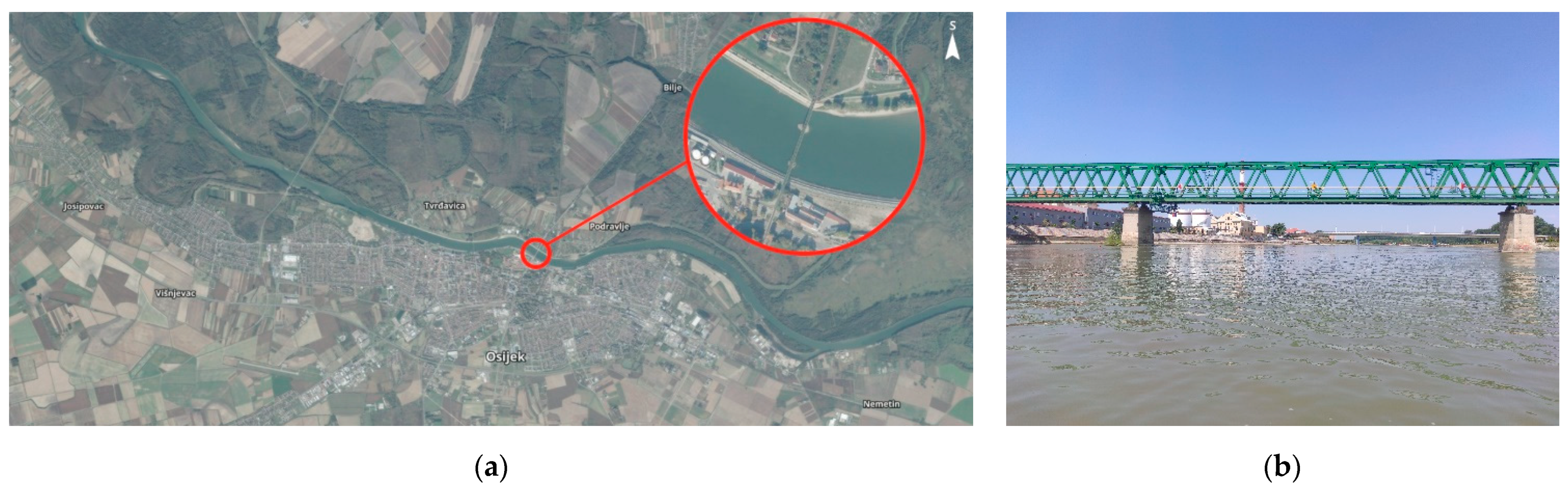
To test the ADVPs’ operation (www.nortekgroup.com (accessed on 9 September 2022)), a scaled model of the Drava River’s reach in Croatia was used as a reference. This Drava River reach was selected because it is the location of the prototype railroad bridge selected for the investigation of scouring around bridge piers protected with riprap [42] under the R3PEAT project [43]. The prototype bridge is located in Osijek, Croatia on the Drava River 18 + 960 km (N 45.56056, E 18.70475, Figure 1). The bridge is a truss bridge with a total of three bridge openings, formed by the two piers located in the main channel and abutments on each riverbank. The largest bridge opening is between the piers—71 m wide—and the symmetrical openings between the piers and the associated abutment are 58 m wide. Two piers are identical (30 m high and 3.5 m wide), with riprap scour protection installed around them.

Figure 1.
Orthophoto map of the case study area (a), photo of the bridge (b).
The flow regime of the Drava River at this river reach is pluvial—glacial, with low flows occurring during winter (January and February) and high flows occurring during spring and summer (May, June and July). The automatic gauging station GS Osijek is located at the river site; it has been operational for almost 200 years (since 1827). The catchment area up to the GS Osijek is 39,982 km2, with a mean long-term water level measured at 85.52 m above sea level (a.s.l.) and a corresponding flow rate of 552 m3/s. The flow conditions at the bridge site were measured with ADCP on three separate campaigns within the various research projects [44,45]. A summary of the measured hydraulic and hydrologic parameters averaged over the entire reach is given in the table (Table 1).

Table 1.
Summary of the measured hydraulic and hydrologic parameters from field surveys.
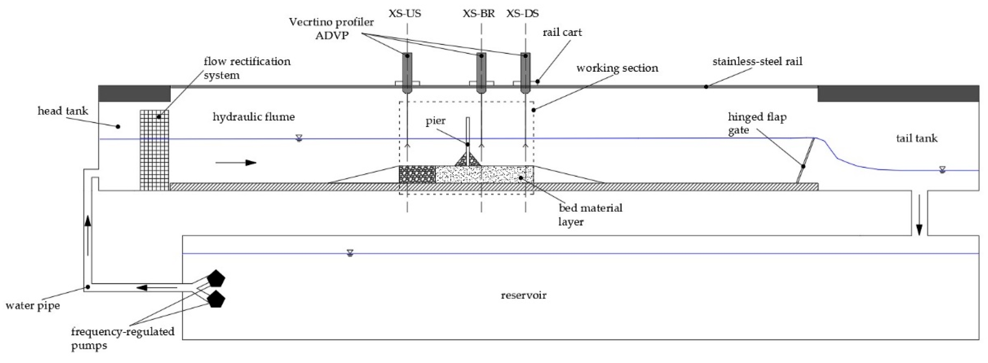
The physical model of the Drava River reach adjacent to the bridge was built in an 18 m-long, 0.9 m-wide and 0.9-m deep recirculating hydraulic flume in the Hydraulics laboratory under the University of Zagreb Faculty of Civil Engineering. The flume has a rectangular cross-section, with sides entirely made of glass for visual monitoring during the experiments, enclosed with inlet and outlet sections and a separate water tank, as shown in the schematic below (Figure 2). The working area of the flume selected for this research to accommodate the sand bed and pier model is 3 m long, 0.4 m wide and 0.8 m deep. The flow rate in the flume is controlled by two frequency-regulated Amarex pumps (www.ksb.com (accessed on 9 September 2022)) with a maximum capacity of ~50 L/s, while the water depth is controlled by a hinged flap gate at the flume outlet. A flow rectification system, aluminum “honeycomb”, is used at the flume inlet to direct the flow coming from the pump into the working section of the flume. Water levels are monitored remotely, obtaining data from two Geolux (www.geolux-radars.com (accessed on 9 September 2022)) LX 80-15 10 Hz Oceanographic Radar Level sensors fitted at the inlet and outlet of the flume’s working section. The model setup—the pier scour physical model scale and velocity measurement—were modelled according to the state-of-the-art literature [35,46,47,48,49,50,51]. The pier was modelled as a distorted scale in the vertical direction—the horizontal scale is 1:125 to the prototype, while the vertical scale is 1:11.18 with the sediment material of the prototype (ρ = 1.65 g/cm3) [52]. According to the Froude similarity principle, the velocity scale is 1:3.34 to the prototype. A bridge pier was included in the model to induce turbulence in the experiment, simulating the conditions occurring in bridge pier turbulence research.
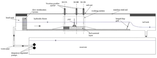
Figure 2.
Scheme of the hydraulic flume setup.
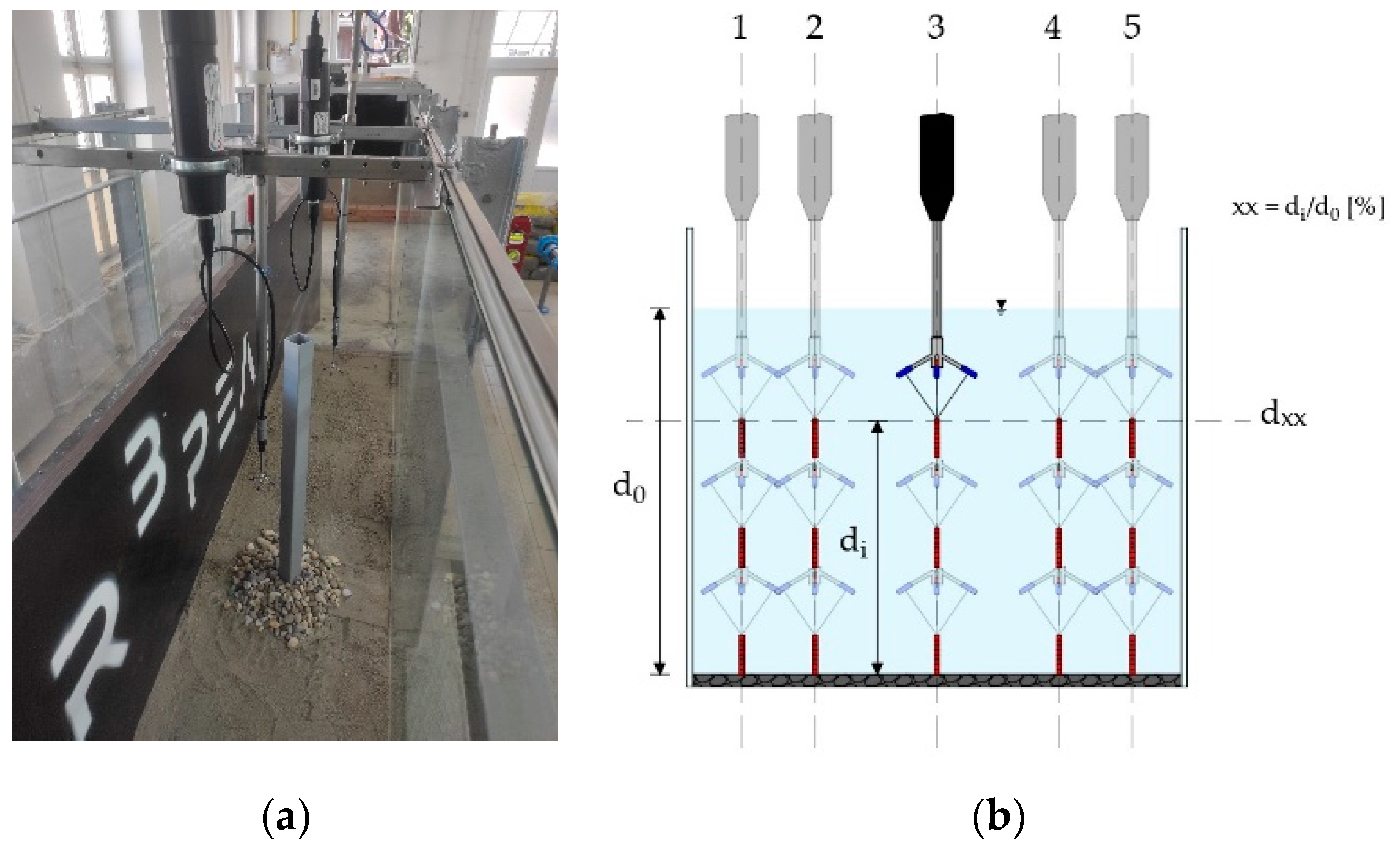
Three-dimensional flow velocity data were measured using an acoustic Doppler velocimeter Vectrino Profiler from Nortek mounted on a mobile rail cart built for the hydraulic flume, which allows it to be placed at predefined measurement positions (Figure 3). The advantage of Nortek’s ADVPs lies in their ability to measure velocity profiles over larger flow depths in contrast to ADVs’ single-point measurement. ADVPs can measure velocity profiles in adjustable cell sizes, from 1 mm to 4 mm in height over a 30 mm range, allowing for investigations of spatial structures of the flow [53]. Another difference between ADVP and ADV is the measurement of two vertical velocity components, with the selection of the appropriate one left to the user. To determine data quality, ADVP provides information on the signal-to-noise ratio and correlation so that the user can filter the data in post-processing in this regard and reduce noise in the signal [54]. The methodological approach adopted for this research was derived from the standard hydrodynamic metrics found in the state-of-the-art review of hydraulics of scour processes around bridge piers. In the comparable studies, velocity was measured at uniformly spaced vertical profiles (~9 cm between profiles) [55], the number of instrument positions was set to measure the velocity profile along the entire flow depth [56] and the measurement duration was ≥60 s [55,57,58], with a sampling frequency of 100 Hz [34,38,56]. For the velocity and depth measurements, a structured raster of measurement points was established for the flow profile, which consisted of points covering the full flume width and depth distributed evenly over the vertical and horizontal measurement axes. Five vertical measurement axes were defined across the flume width, with one central axis and two axes on each side symmetrically distributed towards the flume sidewalls (Figure 3) to cover the entire width of the flume for flow rate calculation [59].

Figure 3.
Photo of the physical model working section and ADVP instruments mounted on a rail cart (a), and scheme of the raster of the measurement points for a single experimental cross-section (b).
ADVP velocity measurements were performed on the three characteristic cross-sections of the model, as presented on the flume scheme. The first cross-section (XS-US) is positioned at the model inlet—the most upstream profile of the working section of the model, representing natural flow conditions in the river. The second cross-section (XS-DS) is positioned at the model outlet—the most downstream profile of the working section of the model, representing flow conditions in the river in a more complex environment due to the influence of the bridge piers on the downstream flow field. The third cross-section (XS-BR) was positioned immediately downstream of the bridge profile, representing the most complex flow conditions in the bridge opening, with wake vortices and recirculation occurring in the pier shadow. The locations of the characteristic cross-sections were selected to reflect both the model setup and the limitations of the flume. The position of the XS-US was selected at the start of the flume’s working section because flow contraction occurs at this point, accelerating and streamlining the flow through the working section. In this section, the flow is contracted, which corresponds well with ADVP measurements since the instrument cannot be placed directly next to the sidewall due to its physical configuration, displacing the first measurement vertical axis 4 cm from the sidewall into the active flow area. The lateral flow contraction increases the streamwise flow velocity component and reduces the spanwise component [60], effectively providing suitable conditions for flow rate measurement [61]. In the contracted cross-section, the recirculating region of the flow is smaller than the downstream [62] and allows for reliable velocity profile extrapolation between the measurement and sidewall. The position of the XS-BR is selected as close as possible to the bridge profile to reflect maximum turbulence conditions, which can be expected for scour applications. The position of the XS-DS corresponds to the end of the flume’s working section, where the flow profile is less disturbed than it is in the bridge profile, but with increased turbulence in comparison to the XS-US. All three cross-sections are representative for the scour experiments—from the approach section, scour location and flow alteration downstream. The selected characteristic cross-sections defined for the flume experiments correspond to the ADCP transects acquired during the field surveys.
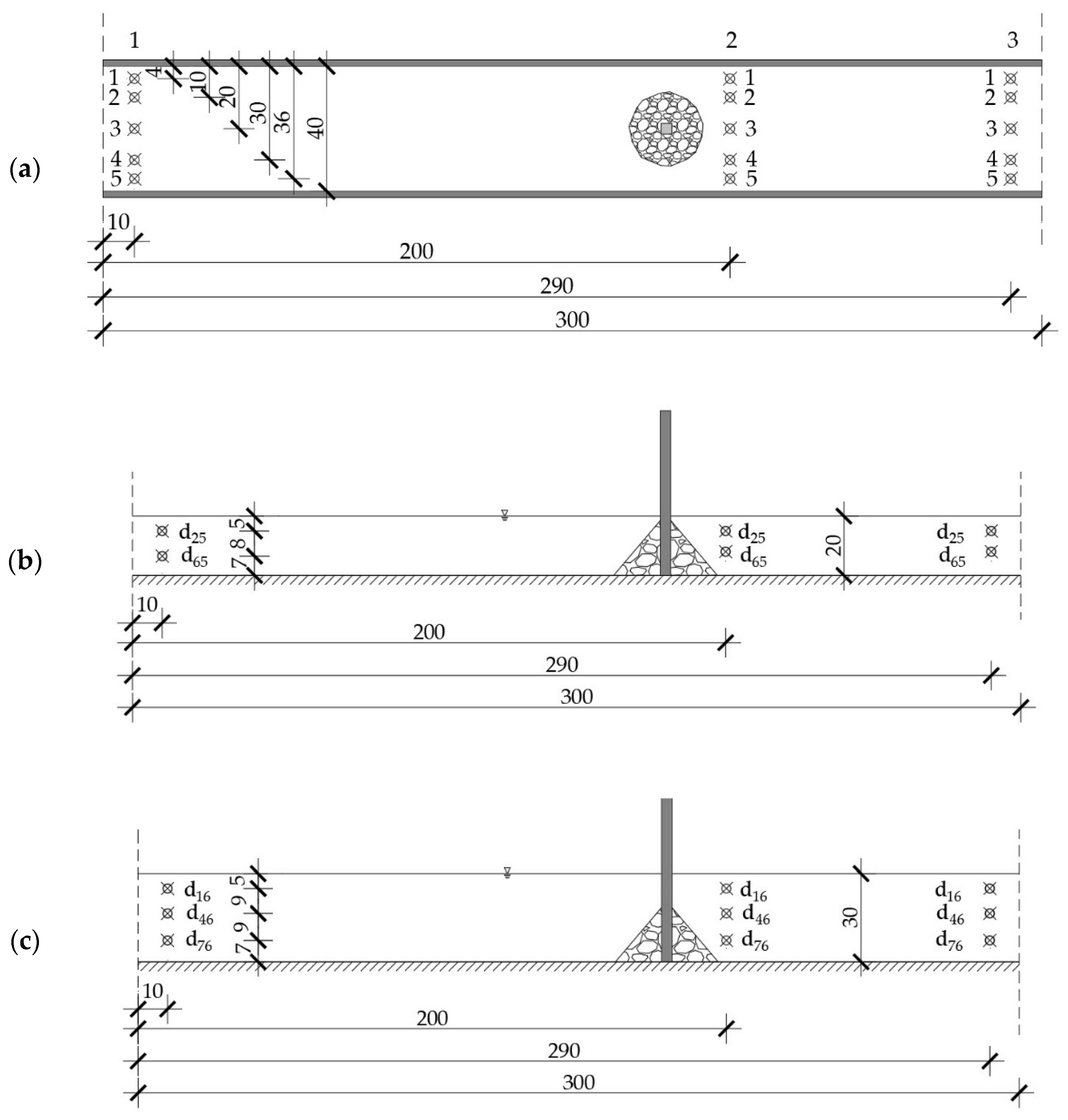
The experimental setup for calibration included a total of four flow scenarios associated with the Drava River flow regime, combining two pump flow rates (20 L/s and 50 L/s) with two flow depths (20 cm and 30 cm). For the velocity and depth measurements, a structured raster of measurement points was established for the flow profile. The raster consisted of points covering the full flume width and depth, distributed evenly over the vertical and horizontal measurement axes. Five vertical measurement axes were defined across the flume width, with one central axis and two axes on each side symmetrically distributed towards the flume sidewalls (Figure 3). The number of horizontal measurement axes is dependent on the flow depth during the experiments—two axes were used for measurements during experiments with a flow depth of 20 cm, and three axes were used for a flow depth of 30 cm (Figure 4).
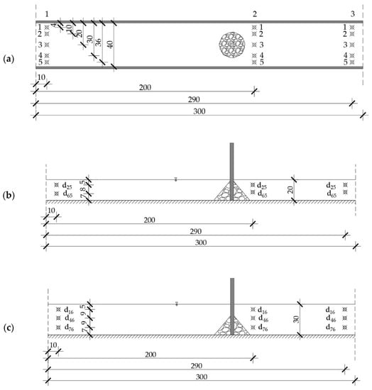
Figure 4.
Flume working section with measurement points: layout (a) and longitudinal profiles for a smaller flow depth (b) and larger flow depth (c), all lengths are given in centimeters.
All velocity measurements were taken at a sampling frequency of 100 Hz in a profiling range of 40–70 mm from the central transducer. Velocities measured by the ADVP were filtered to remove noise from the measured data. The data were filtered by the Phase-Space Thresholding method [63,64], adapted as an algorithm for data pre-processing. The amount of filtered data was significantly below the guidelines suggested by the literature [65]. The operation parameters of Nortek’s ADVPs that can be user-defined are the Ping Algorithm (PA), Transmit Pulse Size (TPS) and Cell Size (CS) [66]. The ping algorithm controls the ping timing parameters to capture the correct velocity—it is varied between Max Interval and Adaptive Interval. Max Interval produces the longest possible ping interval to achieve the correct velocity, while the Adaptive Interval examines the returning echoes and calculates the correct velocity while minimizing acoustic interference. The transmit pulse size indicates the size of the sound wave transmitted through the central transducer, and the cell size determines the spatial resolution of the acquired data. Both the transmit pulse size and the cell size varied between 1 and 4 mm. When all varied parameters are considered, a total of 32 experiments were conducted, as summarized in the table (Table 2).
Table 2.
Configuration of ADVPs’ operation parameters and corresponding flow scenarios used for the experiments.
Once the calibration of the operation parameters is completed, the selected configuration was verified using the field data collected with ADCP surveys. The ADCP data collecting frequency was 3 Hz, collecting flow information in 20 cm bins across the flow depth, combined into one vertical velocity profile—“ensemble”. The verification of the flow velocity profiles measured in the flume was carried out by overlapping the ADVP data collected on vertical measurement axes with the corresponding ADCPs ensemble. During the field survey, ADCP was paired with real-time kinematic positioning (RTK-GPS) device, which provided real-time positioning data for each ensemble. The geolocation enabled the overlapping of the field data with the flume model corresponding to the river section modeled in the laboratory experiments. The differences between ADCP and ADVP data are evaluated using the root-mean-square error (RMSE) of the differences between velocities recorded by the ADCP in a single cell and measured by the ADVP in several cells corresponding to the position within the ADCP cell. The RMSE was calculated over the velocity profiles on the analyzed vertical measurement axes using the following equation:
where: RMSE = root-mean-square error for the analyzed vertical measurement axis [m/s], Vi,ADCP = velocity measured in a single ADCP cell [m/s], Vi,ADVP = velocity measured with ADVP in cells within the corresponding ADCP cell [m/s], N—number of points on the vertical measurement axis.
The verification of the results obtained by ADVP provides new insights into the reliability of the data collected on scaled pier models and provides guidelines for applications in subsequent research.
3. Results and Discussion
3.1. Calibration
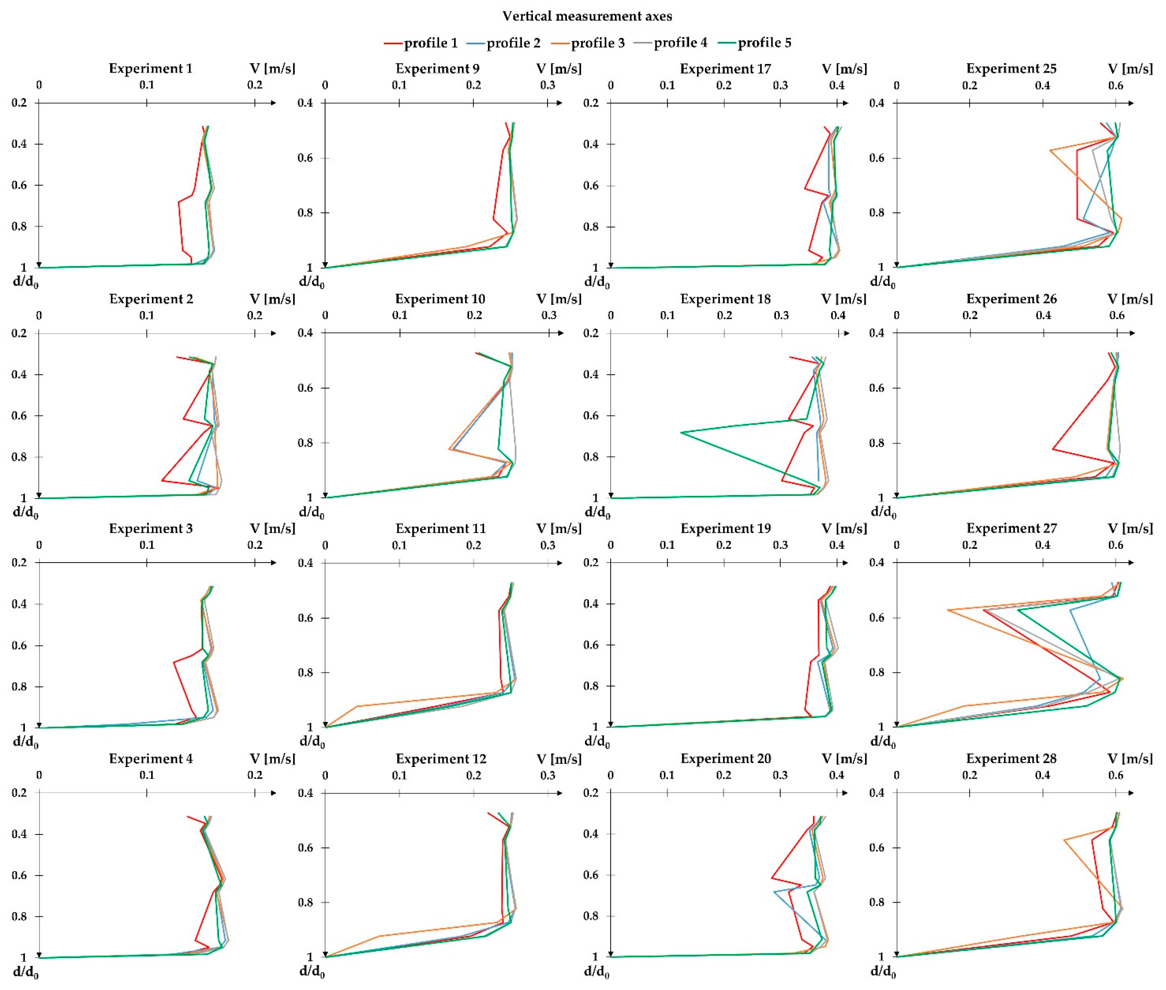
The optimal operation parameters for ADVP were determined as the ones that produce a flow rate through the cross-section equal to the flow rate measured by the flume’s pump. The flume pump is calibrated regularly by the manufacturer as part of the laboratory’s maintenance and is thus considered reliable. During the experiments, the pump was reduced for the larger flow rate to preserve it during long experiments, and, therefore, the flow rate was less than the maximum capacity: ~46 L/s for three flow scenarios and ~49 L/s for the remaining flow scenario. The flow rate through the cross-section is calculated by integrating the flow velocity measured with the ADVP over the active flow area, analogous to the principle used by the ADCP instrument for flow rate calculation. The results for ADVP’s calibration procedure are analyzed separately for all three characteristic cross-sections and across all flow scenarios and the ADVP’s configuration used in the experiments. The following figures (Figure 5 and Figure 6) show the velocity profiles measured for all experiments, given for the XS-US. The figures are composed of a series of four experiments conducted with the same ADVP configuration, depicting the flow velocity profile for each vertical measurement axis.
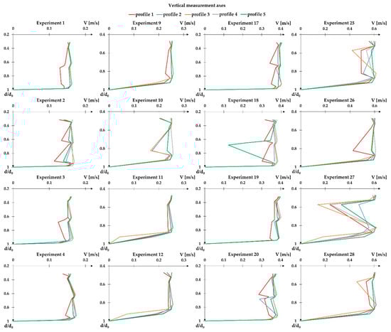
Figure 5.
Composite graph of the flow velocity profile for each vertical measurement axis on XS-US for configurations C1–C4 (from top to bottom).
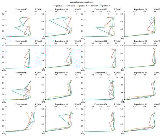
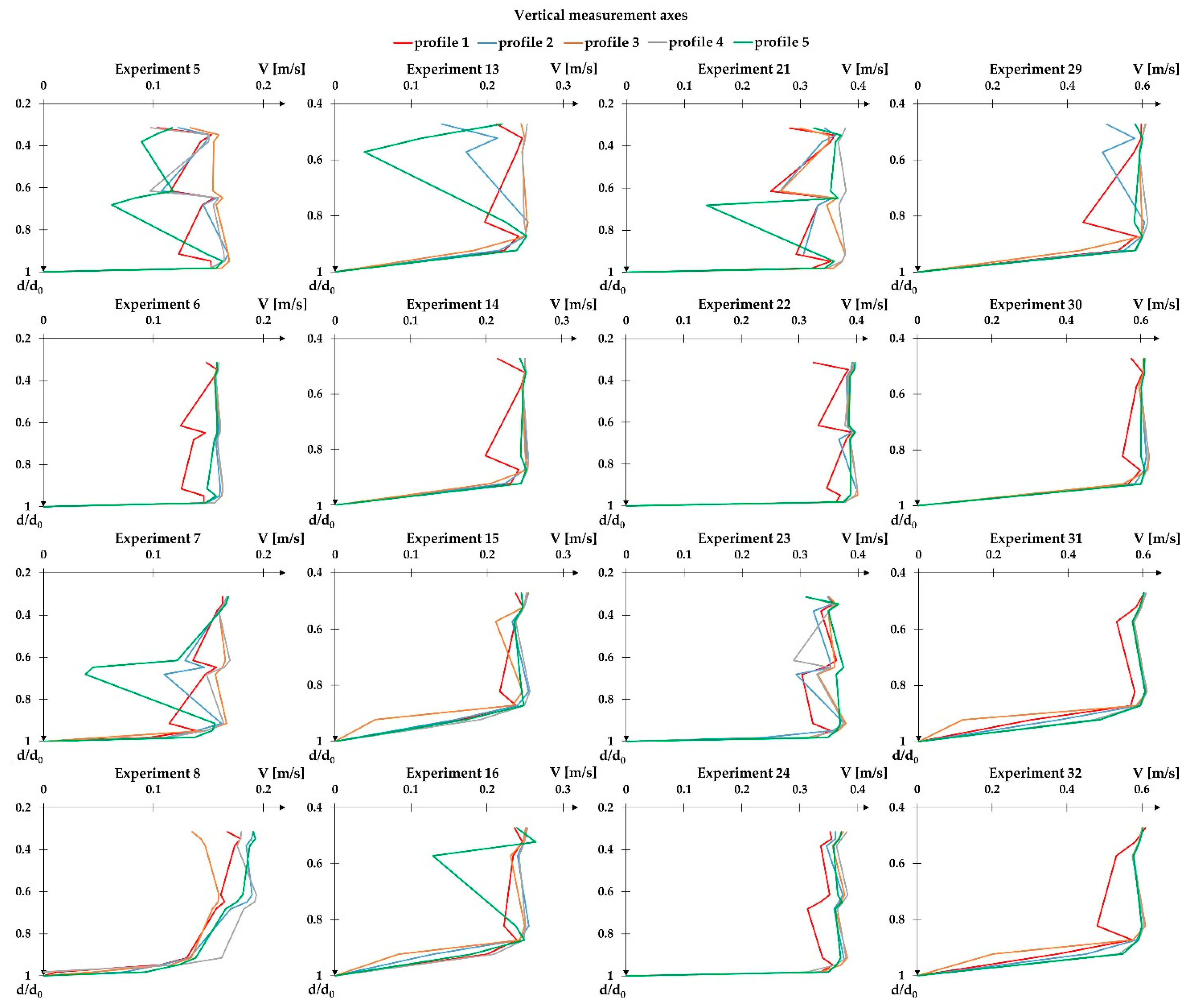
Figure 6.
Composite graph of the flow velocity profile for each vertical measurement axis on XS-US for configurations C5–C8 (from top to bottom).
The results show significant flow velocity profile differences between different configurations. As expected, higher velocities occur at higher flow rates. Common for all measurements is that the flow velocity profiles for configuration in good agreement with the pump flow rate are similar across all vertical measurement axes. For some experiments, vertical 1 deviates from the trend, which is expected, as the model was adjusted to reflect the mild curvature of the river at the model inlet, resulting in smaller velocities next to the left flume wall. The calibration results have shown that the calculated flow rates in the flume correspond best with the pump flow when the ADVP is configured according to the C6 configuration with the following parameters: Ping Algorithm set to Adaptive Interval, Transmit Pulse Size equal to 4 mm and Cell Size of 1 mm (Table 2 and Table 3). This configuration is closest to the pump flow rate for two out of four flow scenarios for the upstream cross-section, with two second best results for the remaining flow scenarios. The results for the downstream cross-section are similar—configuration C6 is the best, second best and third best for two, one and one flow scenario(s), respectively. The second-best overall configuration is shown to be C2, with one best and three third best results for the upstream cross-section and with one best and three second best results for the downstream cross-section. The only difference between the two best configurations is the selection of the Ping Algorithm, with the Adaptive Interval proven to be a more appropriate choice in this research. The configurations that differed the most from the pump flow rates were C5 for the upstream cross-section and C1 and C4 for the downstream cross-section. All three configurations have in common a significant difference between the transmitting pulse size and cell size. Therefore, the optimal configuration for the turbulence measurement around bridge piers is concluded to be configuration C6. Generally, when a relative variation from the pump flow rate is analyzed, all configurations have shown better results for deeper flows (d0 = 30 cm), while for lower flow rates and smaller flow depths (Q = 20 L/s, d0 = 20 cm), relative variations from the pump flow rate were two times higher. The average variation for shallower flows was, on average, 5.5% (ranging between 2.8% and 8.7% for both cross-sections and all four flow scenarios). The average variation for deeper flows was, on average, 4.2% (ranging between 2.1% and 6.6% for both cross-sections and all four flow scenarios.
Table 3.
Summary of the calculated flow rates obtained by the calibration procedure.
3.2. Verification
Following the ADVP calibration, a verification procedure was conducted for the configuration C6 that produced flow rates closest to the pump. The flow scenario used for comparison was Q = ~50 L/s and d0 = 30 cm to satisfy the similarity with the prototype condition measured during the field survey m01 (Table 1). From the ADCP transects spanning across the river’s full width, a subsection corresponding to the flume’s active flow area was extracted to be used in the verification procedure. Specific ensembles within the transects corresponding to the vertical measurement axes used for ADVP measurements (Figure 4) were identified, and flow velocity profile data were extracted. The following figure shows a subsection of the ADCP transect measured at the upstream cross-section, with highlighted ensembles corresponding to the vertical measurement axes 1–5 at the XS-US (Figure 7).

Figure 7.
The subsection of the flow velocity contour profile measured with ADCP and used for verification (m01), corresponding to the model’s XS-US.
When the flow velocity contour profile measured with ADCP, corresponding to the model’s XS-US, is compared between the measurements m01 (Figure 7) and m03 (Figure 8), it can be seen that the flow velocity significantly increases with an increase in the flow rate, while the spatial flow distribution is not affected. In this approach section to the bridge, an increase in the flow rate does not affect the flow velocity distribution in XS-US, and it can be considered that the relative flow field magnitude distribution during floods will not be significantly altered in comparison to the modelled flow environment.
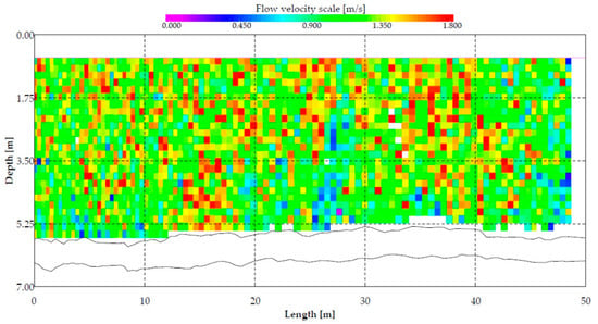
Figure 8.
The subsection of the flow velocity contour profile measured with ADCP during high flows (m03), corresponding to the model’s XS-US.
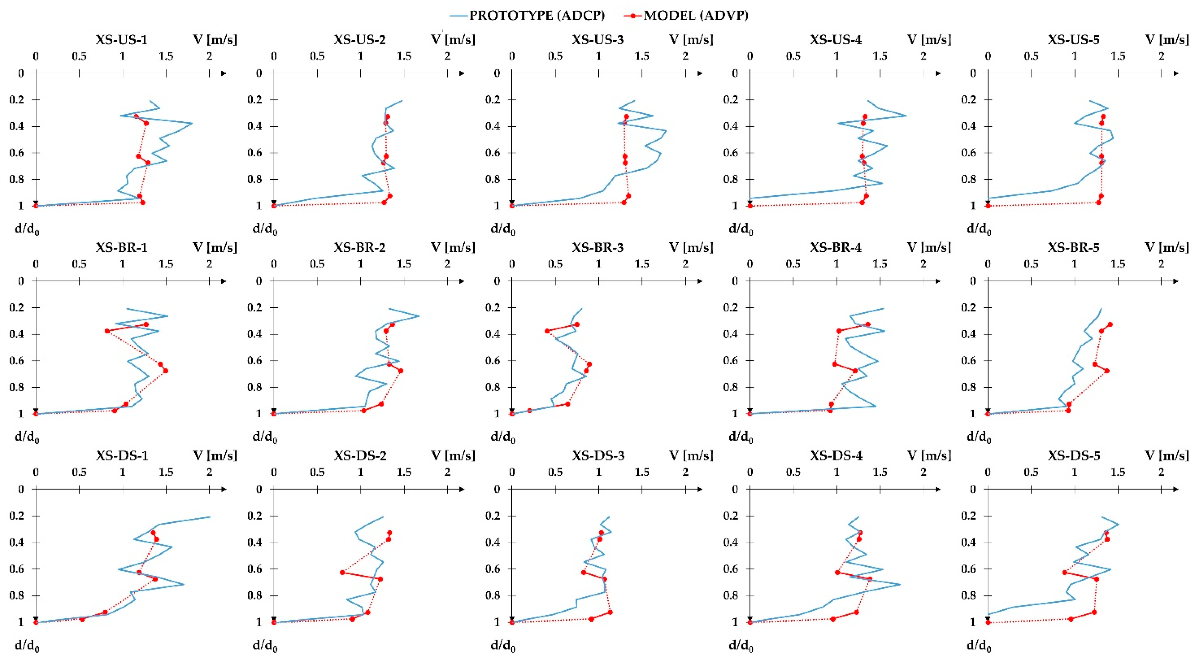
The verification of the ADVP’s data was conducted for the selected ADCP bins corresponding to the location of the ADVP’s cells. Since the cell size used in the experiments was 1 mm, and ADVP can measure 30 mm of the velocity profile, according to the scaling principle used, the entire ADVP velocity profile fits within two ADCP bins. The results for the comparison are given in the following composite figure (Figure 9), composed of flow velocity profiles for each vertical measurement axis (1–5 from left to right) and characteristic cross-section (XS-US, XS-BR and XS-DS from top to bottom, respectively). Flow velocity profiles are presented in the prototype scale [m/s]. The ADCP’s profile covers the entire flow depth, while the ADVP’s profile covers the discrete sections depending on the instrument’s position. The ADVP’s measurements are presented as the average within the depth corresponding to the ADCP bin, thus containing two points per instrument location, connected with a red line. The dotted line connects successive ADVP measurements across the velocity profile section that was not measured.

Figure 9.
Comparison of flow velocity profiles measured for the prototype conditions (ADCP) and experimental conditions (ADVP).
The results show good agreement between the prototype and experimental velocity profiles, having in mind complex flow conditions on this river reach, which are noticeable from the ADCP profiles, which do not resemble the theoretical log-law profile. When the ADVP and ADCP data are compared, it is evident that two successive ADVP points for almost all instances have the same gradient as the corresponding ADCP bins. Velocity profiles measured on the verticals located closer to the left bank and centerline (1, 2 and 3) show good agreement. A larger difference in the measured velocities is present for profiles closer to the right bank (4 and 5), which might be influenced by the model setup. Noticeable differences between velocity profiles are present for the verticals XS-US-3 and XS-BR-4 XS-DS-2. For all vertical measurement axes, there is a visible difference in the ADVP trend of similar velocity magnitudes for the two topmost points, which is not always the case with ADCP data. This trend can be attributed to the more tranquil and streamlined flow in the model, while the flow field of the prototype near the surface can be influenced by secondary current drivers, such as wind or the presence of the survey boat. Additionally, flow velocities measured by the ADCP are shown to be biased close to the ADCP transducer, ranging to more than 25%, as reported by [67,68]. Similar differences are observed near the bottom, where the well-known phenomena of side-lobe interference influence the results, as described in e.g., [69,70,71]. Reynolds stress errors also occur in this area, as reported by Nystrom et al. [41] through the comparison of ADCP and ADV data. Apart from this, the only other noticeable difference that occurs is the mid-section of the measurement verticals XS-BR-2 and XS-BR-4, which are located in the bridge opening. Considering the increased turbulence of this zone influenced by the bridge pier, these results are satisfactory. To quantify the velocity profile similarity between the model and the prototype, the RMSE was calculated for each vertical, as described in the methodology section of the paper. The results are presented in the table (Table 4) for each cross-section.
Table 4.
Calculated RMSE between ADCP and ADVP data.
The RMSE results are consistent across all profiles and measurement vertical axes, with no visible trend. The RMSE values averaged for the entire cross-section have an identical value for the upstream and downstream cross-section (0.14 m/s) and a slightly increased value for the bridge profile (0.144 m/s). This is to be expected considering the complex flow structure through the bridge opening. Both the highest and lowest RMSE values were observed in the bridge profile, with calculated RMSE values of 0.063 m/s and 0.186 m/s for XS-BR-2 and XS-BR-1, respectively. Overall, the RMSE is less than 10% of the averaged ADCP’s ensemble velocity, which is comparable to the findings reported in the literature (e.g., [40,67]). The analyses conducted in this research indicate that flow velocity measurements conducted with ADVP in an experimental model environment can be used to reliably simulate complex flow conditions around the bridge pier and can be subsequently used for scour-related investigations deriving turbulent kinetic energy or Reynolds stress from ADVP velocity fluctuations.
4. Conclusions
The focus of the research presented in this paper was identifying the optimal configuration of the Vectrino Profilers for the measurement of the turbulent flow field around bridge piers. A Drava River reach next to the railroad bridge in Osijek, Croatia was selected as a prototype location, as it is the focus of the R3PEAT project. For this purpose, a scaled model of the river section was set up in the hydraulic flume. A total of 32 laboratory experiments were conducted in the flume, under which instruments’ operation parameters were varied (Ping Algorithm, Transmit Pulse Size and Cell Size) and used for flow velocity profile measurement under a total of four flow scenarios associated with the Drava River flow regime, combining two pump flow rates (20 L/s and 50 L/s) with two flow depths (20 cm and 30 cm). To complement the experimental data, field surveys of the Drava River flow field using ADCP RioGrande were conducted on three separate field campaigns. The determination of the operation parameters was carried out as a two-step process—calibration through the flume’s pump flow rate and verification with ADCP field data.
For the calibration procedure, ADVP data were collected on characteristic profiles—model boundaries. The calibration of the parameters was carried out by integrating the experimental flow velocity data over the cross-section and calculating the flow rate, which, upon successful calibration, corresponds to the flume’s pump flow rate. The results show significant flow velocity profile differences between different instrument configurations. Generally, all configurations have shown better results for deeper flows. The average variation for deeper flows was, on average, 4.2% (ranging between 2.1% and 6.6% for both cross-sections and all four flow scenarios). The calibration results have shown that the calculated flow rates in the flume correspond best with the pump flow when the ADVP is configured according to the C6 configuration with the following parameters: Ping Algorithm set to Adaptive Interval, Transmit Pulse Size equal to 4 mm and Cell Size of 1 mm. This configuration is closest to the pump flow rate for two out of four flow scenarios for both upstream and downstream cross-sections.
For the verification procedure, ADVP data were collected at the model boundaries and, additionally, for the bridge profile representing reference conditions for the bridge scour investigation. Verification of the parameters obtained through calibration was carried out by comparing the ADVP’s velocity profiles with the corresponding profiles measured at the field site with ADCP. The selected characteristic cross-sections defined for the flume experiments correspond to the ADCP transects acquired during the field surveys. The differences between ADCP and ADVP data are evaluated using the root-mean-square error (RMSE) of the differences between velocities recorded by the ADCP in a single cell and measured by the ADVP in several cells corresponding to the position within the ADCP cell. The results show good agreement between the prototype and experimental velocity profiles. When the ADVP and ADCP data are compared, it is evident that two successive ADVP points for almost all instances have the same gradient as the corresponding ADCP bins. A larger difference in the measured velocities is present in the near-bed region and at the surface, which is consistent with the state-of-the-art review and limitations of the ADCP instrument. Overall, the RMSE is less than 10% of the averaged ADCP’s ensemble velocity, which is comparable to the findings reported in the literature.
The analyses conducted in this research indicate that flow velocity measurements conducted with ADVP in an experimental model environment can be used to reliably simulate complex flow conditions around the bridge pier and can subsequently be used for scour-related investigations deriving turbulent kinetic energy or Reynolds stress from ADVP velocity fluctuations. Based on the results, the following setup for ADVP’s operation parameters can be recommended to obtain reliable flow data in the scour hole next to the bridge pier: adaptive Ping Algorithm, Transmit Pulse Size of 4 mm and Cell Size of 1 mm.
Author Contributions
Conceptualization, G.G.; methodology, G.G. and R.F.; software, G.G. and R.F.; validation, R.F.; formal analysis, G.G., R.F. and M.V.; investigation, R.F. and A.H.; data curation, R.F.; writing—original draft preparation, G.G.; writing—review and editing, G.G., R.F., A.H. and M.V.; visualization, G.G. and R.F.; project administration, G.G.; funding acquisition, G.G. All authors have read and agreed to the published version of the manuscript.
Funding
This work has been funded in part by the Croatian Science Foundation under the project R3PEAT (UIP-2019-04-4046).
Institutional Review Board Statement
Not applicable.
Informed Consent Statement
Not applicable.
Data Availability Statement
All data are presented in the main text.
Conflicts of Interest
The authors declare no conflict of interest.
References
- Uotani, T.; Kanda, K.; Michioku, K. Experimental and numerical study on hydrodynamics of riparian vegetation. J. Hydrodyn. Ser. B 2014, 26, 796–806. [Google Scholar] [CrossRef]
- Petrie, J.; Diplas, P.; Gutierrez, M.; Nam, S. Characterizing the mean flow field in rivers for resource and environmental impact assessments of hydrokinetic energy generation sites. Renew. Energy 2014, 69, 393–401. [Google Scholar] [CrossRef]
- Togneri, M.; Lewis, M.; Neill, S.; Masters, I. Comparison of ADCP observations and 3D model simulations of turbulence at a tidal energy site. Renew. Energy 2017, 114, 273–282. [Google Scholar] [CrossRef]
- de Verneil, A.; Rousselet, L.; Doglioli, A.M.; Petrenko, A.A.; Maes, C.; Bouruet-Aubertot, P.; Moutin, T. OUTPACE long duration stations: Physical variability, context of biogeochemical sampling, and evaluation of sampling strategy. Biogeosciences 2018, 15, 2125–2147. [Google Scholar] [CrossRef]
- Dominguez Ruben, L.G.; Szupiany, R.N.; Latosinski, F.G.; López Weibel, C.; Wood, M.; Boldt, J. Acoustic Sediment Estimation Toolbox (ASET): A software package for calibrating and processing TRDI ADCP data to compute suspended-sediment transport in sandy rivers. Comput. Geosci. 2020, 140, 104499. [Google Scholar] [CrossRef]
- Li, K.; Tang, H.; Yuan, S.; Xiao, Y.; Xu, L.; Huang, S.; Rennie, C.D.; Gualtieri, C. A field study of near-junction-apex flow at a large river confluence and its response to the effects of floodplain flow. J. Hydrol. 2022, 610, 127983. [Google Scholar] [CrossRef]
- Carroll, R.W.H.; Warwick, J.J.; James, A.I.; Miller, J.R. Modeling erosion and overbank deposition during extreme flood conditions on the Carson River, Nevada. J. Hydrol. 2004, 297, 1–21. [Google Scholar] [CrossRef]
- Ottevanger, W.; Blanckaert, K.; Uijttewaal, W.S.J. Processes governing the flow redistribution in sharp river bends. Geomorphology 2012, 163, 45–55. [Google Scholar] [CrossRef]
- Bombar, G.; Cardoso, A.H. Effect of the sediment discharge on the equilibrium bed morphology of movable bed open-channel confluences. Geomorphology 2020, 367, 107329. [Google Scholar] [CrossRef]
- Parsons, D.R.; Jackson, P.R.; Czuba, J.A.; Engel, F.L.; Rhoads, B.L.; Oberg, K.A.; Best, J.L.; Mueller, D.S.; Johnson, K.K.; Riley, J.D. Velocity Mapping Toolbox (VMT): A processing and visualization suite for moving-vessel ADCP measurements. Earth Surf. Processes Landf. 2013, 38, 1244–1260. [Google Scholar] [CrossRef]
- Moore, S.A.; Le Coz, J.; Hurther, D.; Paquier, A. On the application of horizontal ADCPs to suspended sediment transport surveys in rivers. Cont. Shelf Res. 2012, 46, 50–63. [Google Scholar] [CrossRef]
- Mercier, P.; Thiébaut, M.; Guillou, S.; Maisondieu, C.; Poizot, E.; Pieterse, A.; Thiébot, J.; Filipot, J.-F.; Grondeau, M. Turbulence measurements: An assessment of Acoustic Doppler Current Profiler accuracy in rough environment. Ocean. Eng. 2021, 226, 108819. [Google Scholar] [CrossRef]
- Miller, C.T.; Dawson, C.N.; Farthing, M.W.; Hou, T.Y.; Huang, J.; Kees, C.E.; Kelley, C.T.; Langtangen, H.P. Numerical simulation of water resources problems: Models, methods, and trends. Adv. Water Resour. 2013, 51, 405–437. [Google Scholar] [CrossRef]
- Pham Van, C.; Deleersnijder, E.; Bousmar, D.; Soares-Frazão, S. Simulation of flow in compound open-channel using a discontinuous Galerkin finite-element method with Smagorinsky turbulence closure. J. Hydro-Environ. Res. 2014, 8, 396–409. [Google Scholar] [CrossRef]
- Peruzzi, C.; Poggi, D.; Ridolfi, L.; Manes, C. On the scaling of large-scale structures in smooth-bed turbulent open-channel flows. J. Fluid Mech. 2020, 889, A1. [Google Scholar] [CrossRef]
- Ali, S.Z.; Dey, S. Origin of the scaling laws of sediment transport. Proceedings of the Royal Society A: Mathematical. Phys. Eng. Sci. 2017, 473, 20160785. [Google Scholar] [CrossRef]
- Valyrakis, M.; Latessa, G.; Koursari, E.; Cheng, M. Floodopoly: Enhancing the Learning Experience of Students in Water Engineering Courses. Fluids 2020, 5, 21. [Google Scholar] [CrossRef]
- García, C.M.; Cantero, M.I.; Niño, Y.; García, M.H. Acoustic Doppler Velocimeters (ADV) Performance Curves (APCs) Sampling the Flow Turbulence. In Proceedings of the World Water and Environmental Resources Congress, Salt Lake City, GA, USA, 27 June–1 July 2004. [Google Scholar] [CrossRef]
- Scharnowski, S.; Bross, M.; Kähler, C.J. Accurate turbulence level estimations using PIV/PTV. Exp. Fluids 2018, 60, 1. [Google Scholar] [CrossRef]
- Thomas, R.E.; Schindfessel, L.; McLelland, S.J.; Creëlle, S.; De Mulder, T. Bias in mean velocities and noise in variances and covariances measured using a multistatic acoustic profiler: The Nortek Vectrino Profiler. Meas. Sci. Technol. 2017, 28, 075302. [Google Scholar] [CrossRef]
- Leng, X.; Chanson, H. Unsteady velocity profiling in bores and positive surges. Flow Meas. Instrum. 2017, 54, 136–145. [Google Scholar] [CrossRef]
- Baghalian, S.; Ghodsian, M. Experimental study on the effects of artificial bed roughness on turbidity currents over abrupt bed slope change. Int. J. Sediment Res. 2020, 35, 256–268. [Google Scholar] [CrossRef]
- Wang, X.Y.; Yang, Q.Y.; Lu, W.Z.; Wang, X.K. Experimental study of near-wall turbulent characteristics in an open-channel with gravel bed using an acoustic Doppler velocimeter. Exp. Fluids 2012, 52, 85–94. [Google Scholar] [CrossRef]
- Gilja, G.; Ocvirk, E.; Fliszar, R. Experimental Investigation of the Reynolds Shear Stress Exceedance Rate for the Injury and Disorientation Biocriteria Boundary in the Pool-Orifice and Vertical Slot Type Fishways. Appl. Sci. 2021, 11, 7708. [Google Scholar] [CrossRef]
- Gilja, G.; Ocvirk, E.; Cikojević, A. Experimental investigation of flow field in a physical fishway model. In Proceedings of the 16th International symposium Water Management & Hydraulic Engineering WMHE 2019, Skopje, North Macedonia, 5–7 September 2019. [Google Scholar]
- Caroppi, G.; Västilä, K.; Gualtieri, P.; Järvelä, J.; Giugni, M.; Rowiński, P.M. Acoustic Doppler velocimetry (ADV) data on flow-vegetation interaction with natural-like and rigid model plants in hydraulic flumes. Data Brief 2020, 32, 106080. [Google Scholar] [CrossRef] [PubMed]
- Sarker, M.A. Flow measurement around scoured bridge piers using Acoustic-Doppler Velocimeter (ADV). Flow Meas. Instrum. 1998, 9, 217–227. [Google Scholar] [CrossRef]
- Maity, H.; Mazumder, B.S. Prediction of plane-wise turbulent events to the Reynolds stress in a flow over scour-bed. Environmetrics 2017, 28, e2442. [Google Scholar] [CrossRef]
- Canilho, H.; Santos, C.; Taborda, C.; Falorca, I.; Fael, C. Measurements of suspended ashes concentration in turbulent flow with acoustic doppler velocimeter. Flow Meas. Instrum. 2022, 87, 102207. [Google Scholar] [CrossRef]
- Chmiel, O.; Baselt, I.; Malcherek, A. Applicability of Acoustic Concentration Measurements in Suspensions of Artificial and Natural Sediments Using an Acoustic Doppler Velocimeter. Acoustics 2019, 1, 6. [Google Scholar] [CrossRef]
- Mosquera, R.; Pedocchi, F. Salinity estimation from Acoustic Doppler Velocimeter measurements. Cont. Shelf Res. 2019, 180, 59–62. [Google Scholar] [CrossRef]
- Zedel, L.; Hay, A. Turbulence measurements in a jet: Comparing the Vectrino and Vectrino II. In Proceedings of the IEEE/OES Tenth Working Conference on Current, Waves and Turbulence Measurement, Monterey, CA, USA, 20–23 March 2011. [Google Scholar]
- Voulgaris, G.; Trowbridge, J.H. Evaluation of the Acoustic Doppler Velocimeter (ADV) for Turbulence Measurements. J. Atmos. Ocean. Technol. 1998, 15, 272–289. [Google Scholar] [CrossRef]
- Craig, R.G.A.; Loadman, C.; Clement, B.; Rusello, P.J.; Siegel, E. Characterization and testing of a new bistatic profiling acoustic Doppler velocimeter: The Vectrino-II. In Proceedings of the IEEE/OES Tenth Working Conference on Current, Waves and Turbulence Measurement, Monterey, CA, USA, 20–23 March 2011. [Google Scholar]
- Lacey, J.; Duguay, J.; MacVicar, B. Comparison of velocity and turbulence profiles obtained with a Vectrino Profiler and PIV. E3S Web Conf. 2018, 40, 05070. [Google Scholar] [CrossRef]
- Ruonan, B.; Liekai, C.; Xingkui, W.; Danxun, L. Comparison of ADV and PIV Measurements in Open Channel Flows. Procedia Eng. 2016, 154, 995–1001. [Google Scholar] [CrossRef]
- Koca, K.; Noss, C.; Anlanger, C.; Brand, A.; Lorke, A. Performance of the Vectrino Profiler at the sediment–water interface. J. Hydraul. Res. 2017, 55, 573–581. [Google Scholar] [CrossRef]
- Jourdain de Thieulloy, M.; Dorward, M.; Old, C.; Gabl, R.; Davey, T.; Ingram, D.M.; Sellar, B.G. On the Use of a Single Beam Acoustic Current Profiler for Multi-Point Velocity Measurement in a Wave and Current Basin. Sensors 2020, 20, 3881. [Google Scholar] [CrossRef] [PubMed]
- Stone, M.C.; Hotchkiss, R.H. Evaluating velocity measurement techniques in shallow streams. J. Hydraul. Res. 2007, 45, 752–762. [Google Scholar] [CrossRef]
- Nidzieko, N.J.; Fong, D.A.; Hench, J.L. Comparison of Reynolds Stress Estimates Derived from Standard and Fast-Ping ADCPs. J. Atmos. Ocean. Technol. 2005, 23, 854–861. [Google Scholar] [CrossRef]
- Nystrom Elizabeth, A.; Rehmann Chris, R.; Oberg Kevin, A. Evaluation of Mean Velocity and Turbulence Measurements with ADCPs. J. Hydraul. Eng. 2007, 133, 1310–1318. [Google Scholar] [CrossRef]
- Harasti, A.; Gilja, G.; Potočki, K.; Lacko, M. Scour at Bridge Piers Protected by the Riprap Sloping Structure: A Review. Water 2021, 13, 3606. [Google Scholar] [CrossRef]
- Gilja, G.; Cikojević, A.; Potočki, K.; Varga, M.; Adžaga, N. Remote Real-time Riprap Protection Erosion AssessmenT on large rivers. In Proceedings of the EGU General Assembly 2020, Wien, Austria, 4–8 May 2020. [Google Scholar] [CrossRef]
- Gilja, G.; Bekić, D.; Kuspilić, N. Comparison of flow velocity vectors collected by using RTK-GPS and bottom-tracking as a reference on a boat mounted ADCP. In Current Events in Hydraulic Engineering; Sawicki, J.M., Zima, P., Eds.; Gdansk University of Technology: Gdansk, Poland, 2011; pp. 123–135. [Google Scholar]
- Gilja, G.; Kuspilić, N. Modeling of long-term sedimentation in the Osijek port basin. In Proceedings of the 14th International Symposium on Water Management and Hydraulic Engineering, Brno, Czech Republic, 8–10 September 2015. [Google Scholar]
- Tabarestani, M.K.; Salamatian, S.A. Physical modelling of local scour around bridge pier. Malays. J. Civ. Eng. 2016, 28, 349–364. [Google Scholar]
- Waldron, R.L. Physical Modeling of Flow and Sediment Transport Using Distorted Scale Modeling. Master’s Thesis, Tulane University, New Orleans, LA, USA, May 2008. [Google Scholar]
- Sutherland, J.; Soulsby, R.L. Guidelines for physical modelling of mobile sediments. In Proceedings of the Third International Conference on the Application of Physical Modelling to Port and Coastal Protection, Barcelona, Spain, 28 September–1 October 2010. [Google Scholar]
- Link, O.; Henríquez, S.; Ettmer, B. Physical scale modelling of scour around bridge piers. J. Hydraul. Res. 2019, 57, 227–237. [Google Scholar] [CrossRef]
- Kirkegaard, J.; Wolters, G.; Sutherland, J.; Soulsby, R.; Frostick, L.; McLelland, S.; Mercer, T.; Gerritsen, H. Users Guide to Physical Modelling and Experimentation, 1st ed.; CRC Press: London, UK, 2011; p. 272. [Google Scholar]
- Thomas, R.E.; McLelland, S.J. The impact of macroalgae on mean and turbulent flow fields. J. Hydrodyn. Ser. B 2015, 27, 427–435. [Google Scholar] [CrossRef]
- Fliszar, R.; Gilja, G.; Harasti, A.; Potočki, K. Scaling approach for physical modelling of pier scour. In Proceedings of the EGU General Assembly 2021, Wien, Austria, 19–30 April 2021. [Google Scholar] [CrossRef]
- Bagherimiyab, F.; Lemmin, U. Large-scale coherent flow structures in rough-bed open-channel flow observed in fluctuations of three-dimensional velocity, skin friction and bed pressure. J. Hydraul. Res. 2018, 56, 806–824. [Google Scholar] [CrossRef]
- Hurther, D.; Lemmin, U. A Correction Method for Turbulence Measurements with a 3D Acoustic Doppler Velocity Profiler. J. Atmos. Ocean. Technol. 2001, 18, 446–458. [Google Scholar] [CrossRef]
- Graf, W.H.; Istiarto, I. Flow pattern in the scour hole around a cylinder. J. Hydraul. Res. 2002, 40, 13–20. [Google Scholar] [CrossRef]
- Duma, D.; Erpicum, S.; Archambeau, P.; Pirotton, M.; Dewals, B. Velocity and Turbulence Measurements for Assessing the Stability of Riverbeds: A Comparison between UVP and ADVP. In Proceedings of the 11th International Conference on Hydroscience & Engineering ICHE 2014, Hamburg, Germany, 28 September–2 October 2014; pp. 539–544. [Google Scholar]
- Kurniawan, A.; Altinakar, M.S. Velocity and turbulence measurements in a scour hole using an Acoustic Doppler Velocity Profiler. In Proceedings of the Third International Symposium on Ultrasonic Doppler Methods for Fluid Mechanics and Fluid Engineering 3rd ISUD, Lausanne, Switzerland, 9–11 September 2002; pp. 37–43. [Google Scholar]
- Groom, J.; Friedrich, H. Spatial structure of near-bed flow properties at the grain scale. Geomorphology 2019, 327, 14–27. [Google Scholar] [CrossRef]
- Meral, R.; Degirmenci, H.; Gençoglan, C.; Akyüz, A.; Sesveren, S. Measuring Water Flow Velocity and Discharge with Acoustic Doppler Velocimeter (ADV). In Proceedings of the International Meeting on Soil Fertility Land Management and Agroclimatology, Urfa, Turkey, 29–31 October 2008. [Google Scholar]
- Rehman, K.; Hong, S.H. Influence of lateral flow contraction on bed shear stress estimation by using measured turbulent kinetic energy. Exp. Therm. Fluid Sci. 2022, 139, 110742. [Google Scholar] [CrossRef]
- Ribeiro, Á.S.; Alves e Sousa, J.; Simões, C.; Lages Martins, L.; Dias, L.; Mendes, R.; Martins, C. Parshall flumes flow rate uncertainty including contributions of the model parameters and correlation effects. Meas. Sens. 2021, 18, 100108. [Google Scholar] [CrossRef]
- Chrisohoides, A.; Sotiropoulos, F.; Sturm Terry, W. Coherent Structures in Flat-Bed Abutment Flow: Computational Fluid Dynamics Simulations and Experiments. J. Hydraul. Eng. 2003, 129, 177–186. [Google Scholar] [CrossRef]
- Goring, D.G.; Nikora, V.I. Despiking Acoustic Doppler Velocimeter Data. J. Hydraul. Eng. 2002, 128, 117–126. [Google Scholar] [CrossRef]
- Wahl, T.L. “Discussion of Despiking Acoustic Doppler Velocimeter Data” by Derek G. Goring and Vladimir I. Nikora. J. Hydraul. Eng. 2003, 129, 484–487. [Google Scholar] [CrossRef]
- Martin, V.; Fisher, T.S.R.; Millar, R.G.; Quick, M.C. ADV Data Analysis for Turbulent Flows: Low Correlation Problem. In Proceedings of the Hydraulic Measurements and Experimental Methods Specialty Conference, Estes Park, CO, USA, 28 July–1 August 2002. [Google Scholar]
- NORTEK. The Comprehensive Manual for Velocimeters; NORTEK AS: Rud, Norway, 2018; p. 119. [Google Scholar]
- Mueller, D.S.; Abad, J.D.; García, C.M.; Gartner, J.W.; García, M.H.; Oberg, K.A. Errors in Acoustic Doppler Profiler Velocity Measurements Caused by Flow Disturbance. J. Hydraul. Eng. 2007, 133, 1411–1420. [Google Scholar] [CrossRef]
- Gartner, J.W.; Ganju, N.K. A Preliminary Evaluation of Near-Transducer Velocities Collected with Low-Blank Acoustic Doppler Current Profiler. In Proceedings of the Hydraulic Measurements and Experimental Methods, Estes Park, CO, USA, 28 July–1 August 2002. [Google Scholar]
- Simpson, M.R. Discharge Measurements Using a Broad-Band Acoustic Doppler Current Profiler; U.S. Geological Survey: Sacramento, CA, USA, 2001; p. 40.
- Mueller, D.S.; Wagner, C.R. Measuring Discharge with Acoustic Doppler Current Profilers from a Moving Boat; U.S. Geological Survey: Reston, VA, USA, 2009; p. 72.
- Liu, D.; Al-Obaidi, K.; Valyrakis, M. The assessment of an Acoustic Doppler Velocimetry profiler from a user’s perspective. Acta Geophys. 2022. [Google Scholar] [CrossRef]


Publisher’s Note: MDPI stays neutral with regard to jurisdictional claims in published maps and institutional affiliations. |
© 2022 by the authors. Licensee MDPI, Basel, Switzerland. This article is an open access article distributed under the terms and conditions of the Creative Commons Attribution (CC BY) license (https://creativecommons.org/licenses/by/4.0/).