Article

Data-Driven Reduced-Order Modeling of Convective Heat Transfer in Porous Media

1
Department of Nuclear Engineering, Texas A&M University, 423 Spence St, College Station, TX 77843, USA
2
Laboratory of Reactor Physics and Systems Behaviour, École Polytechnique Fédérale de Lausanne, PH D3 465 (Batiment PH), Station 3, CH-1015 Lausanne, Switzerland
*
Author to whom correspondence should be addressed.
Fluids 2021, 6(8), 266; https://doi.org/10.3390/fluids6080266
Submission received: 29 June 2021 / Revised: 15 July 2021 / Accepted: 19 July 2021 / Published: 28 July 2021
(This article belongs to the Special Issue Reduced Order Models for Computational Fluid Dynamics)

Abstract

:
This work presents a data-driven Reduced-Order Model (ROM) for parametric convective heat transfer problems in porous media. The intrusive Proper Orthogonal Decomposition aided Reduced-Basis (POD-RB) technique is employed to reduce the porous medium formulation of the incompressible Reynolds-Averaged Navier–Stokes (RANS) equations coupled with heat transfer. Instead of resolving the exact flow configuration with high fidelity, the porous medium formulation solves a homogenized flow in which the fluid-structure interactions are captured via volumetric flow resistances with nonlinear, semi-empirical friction correlations. A supremizer approach is implemented for the stabilization of the reduced fluid dynamics equations. The reduced nonlinear flow resistances are treated using the Discrete Empirical Interpolation Method (DEIM), while the turbulent eddy viscosity and diffusivity are approximated by adopting a Radial Basis Function (RBF) interpolation-based approach. The proposed method is tested using a 2D numerical model of the Molten Salt Fast Reactor (MSFR), which involves the simulation of both clean and porous medium regions in the same domain. For the steady-state example, five model parameters are considered to be uncertain: the magnitude of the pumping force, the external coolant temperature, the heat transfer coefficient, the thermal expansion coefficient, and the Prandtl number. For transient scenarios, on the other hand, the coastdown-time of the pump is the only uncertain parameter. The results indicate that the POD-RB-ROMs are suitable for the reduction of similar problems. The relative L2 errors are below 3.34% for every field of interest for all cases analyzed, while the speedup factors vary between 54 (transient) and 40,000 (steady-state).

1. Introduction

The simulation of fluid flows is essential in many engineering fields. For this, high-fidelity models using Computational Fluid Dynamics (CFD) are commonly employed to numerically solve the Navier–Stokes equations on two- or three-dimensional domains. These CFD models are often computationally expensive; therefore, they are not adapted for multi-query applications, such as uncertainty quantification or design optimization, where numerous solutions are needed for various model/input parameter values. Model-Order Reduction (MOR) techniques can lower the computational burden of such applications by the generation of Reduced-Order Models (ROMs), which are considerably faster to solve.
Thermal-hydraulic system codes serve as good examples for ROMs since the Navier–Stokes equations are simplified to one- or zero-dimensional equations by solving for surface or volume averaged values of the variables [1,2,3]. These reduced models are often referred to as physics-based ROMs and are commonly used for the analysis of industrial systems [4,5,6]. A disadvantage of these codes is that they often struggle with the modeling of multi-dimensional effects in larger fluid volumes (flow detachments, recirculation, etc.).
For this reason, a new research direction has emerged in the fluid dynamics community with the goal of generating models that can handle local effects and still be significantly faster than conventional CFD. One of these approaches is the porous medium treatment of zones with complex structural elements. In these models, the elements are homogenized into porous medium zones, and the interactions between the fluid and the homogenized structures are handled using semi-empirical correlation functions [7,8].
These models solve the Porous Medium Navier–Stokes (PMNS) equations [7,9], which simplify complex structures into coarse-mesh porous medium zones. However, a large number of computational cells may still be necessary to resolve the homogenized flow problem, which makes the porous medium approach impractical when multi-query applications are considered. For this reason, this paper aims at the development of a data-driven ROM, which can further reduce the computational cost of solving the PMNS equations.
The intrusive Proper Orthogonal Decomposition aided Reduced-Basis method [10,11,12,13] belongs to a family of data-driven ROM techniques, in the sense that some information is needed a priori about the solution manifold. This information is collected using the method of snapshots [11], which involves the execution of a high-fidelity model and capturing snapshots of the solution fields at different time instances and model parameter values. Then, global spatial basis functions are obtained for the solution fields by compressing the information in the snapshots using POD.
These global spatial basis functions (or POD modes) are used to approximate the solution and, through a Galerkin projection, to reduce the number of unknowns in the numerical models. POD-RB for clean fluid flow problems have already been investigated for finite element [14,15,16] and finite volume [17,18,19,20] spatial discretizations. The method has been applied to turbulent fluid flows [17,21,22] and coupled fluid dynamics and enthalpy equations [22,23]. Recently, studies have shown that industry-standard performances can be achieved in coupled fluid dynamics- heat exchange problems using POD-RB [16].
Other, non-intrusive, purely data-driven machine learning approaches have also been developed for the reduction of problems involving fluid flows. Some examples include Smolyak sparse grid interpolation [24], Radial Basis Function (RBF) interpolation [25], and neural networks [26]. The common feature of these methods is that they treat the function describing the behavior of the system as a black box and attempt to approximate it using the already available input–output data pairs. On the other hand, the proposed intrusive POD-RB-ROM is physics-based meaning that it incorporates the knowledge of the differential operators in the reduced model. Due to this feature, the proposed ROM has the potential to use fewer training samples for a given accuracy.
Furthermore, the utilization of intrusive POD-RB ROMs for porous medium flows has also been investigated in [27,28,29]. However, these works focus on slow flows in dense porous media as described by Darcy’s law, which neglect the nonlinear inertial term in the PMNS equations. Other reduction techniques, such as reduced-basis methods with predefined spatial profiles [30] and Smolyak sparse grid interpolation [31] have also been successfully applied to the multiphase Darcy equation to investigate thermal instabilities and to simulate petroleum reservoirs.
In this work, however, advection-driven fluid flows are considered in closed-loop systems with porous medium zones. Therefore, the complete PMNS equations are solved and reduced using POD-RB. This contribution, to the best of the authors’ knowledge, is novel in the reduced-order modeling community. We also note that some recent work has focused on the coupling between POD-RB-ROMs and thermal-hydraulics system codes [32] and can be an alternative to the work presented here.
The rest of the paper is organized as follows. In Section 2, we review the necessary steps in the generation of the POD-RB-ROMs for problems involving convective heat transfer in porous media. Then, in Section 3, two numerical examples are presented using a 2D model of the Molten Salt Fast Reactor (MSFR) [33], which showcases a thermal-hydraulics system in nuclear engineering that includes both clean fluid and porous medium zones. Lastly, Section 4 discusses the results, while Section 5 draws our conclusions and proposes further improvements for the method in this paper.

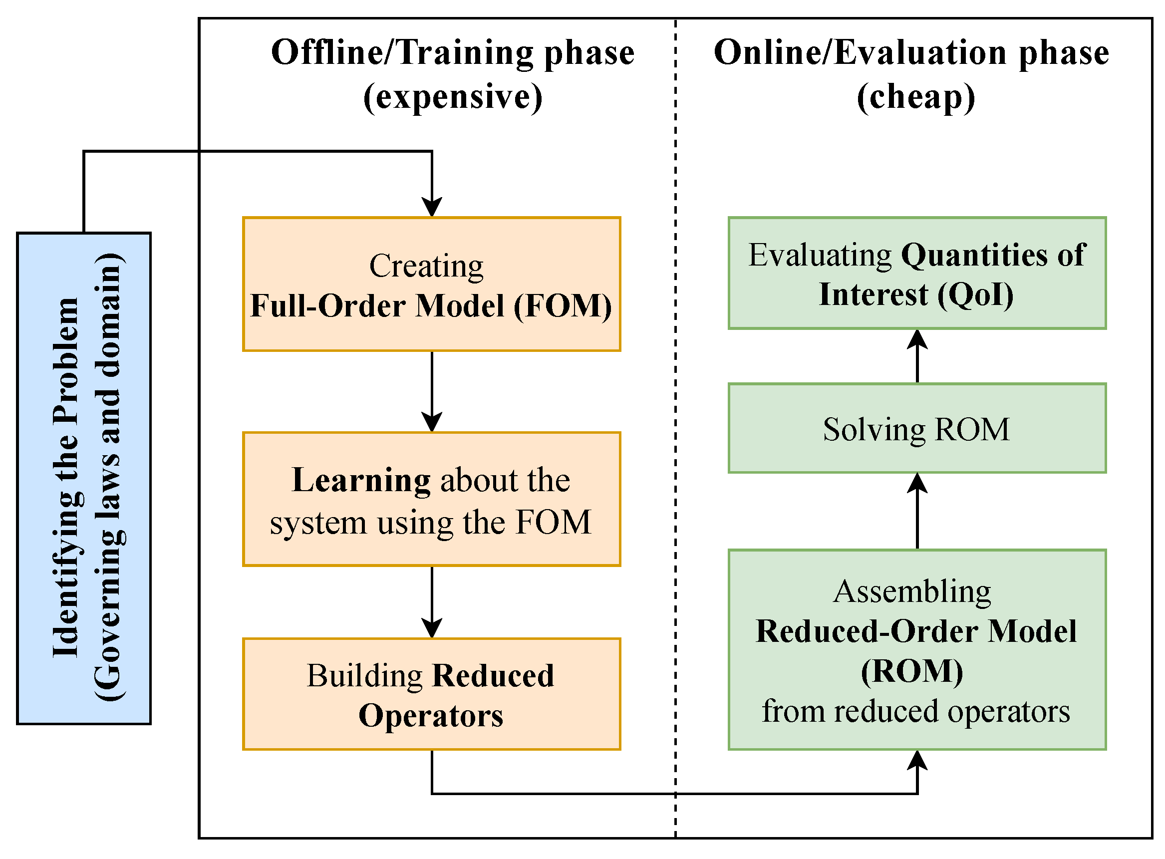
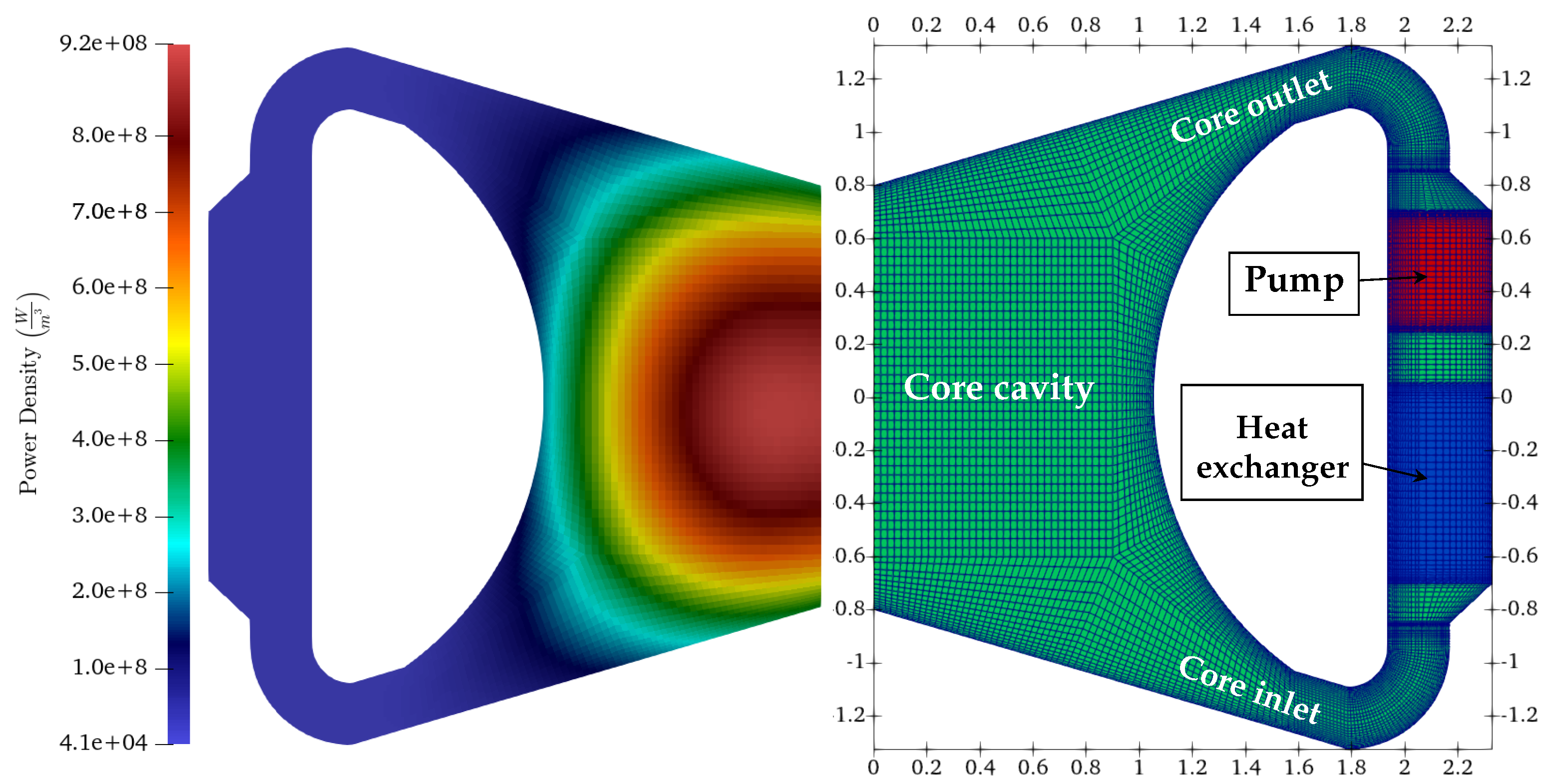
2. Materials and Methods

In this work, a Proper Orthogonal Decomposition aided Reduced-Basis (POD-RB) technique is developed for the parametric Model Order Reduction (MOR) of hydraulic systems where the structural elements are homogenized and treated as porous media. The flow chart of the MOR process is presented in Figure 1. It starts with the identification of the governing laws for the fluid flow on a specific domain with appropriate boundary conditions.
Then, we enter the training phase, which requires the generation of a Full-Order Model (FOM) by the discretization of the previously selected governing equations. Following this, the FOM is exercised to collect information about the parameter- and time-dependent solution manifold. The acquired information is then synthesized in reduced operators. This concludes the training phase, which is computationally expensive since it requires several solutions of the FOM.
The process continues with the online phase, which consists of the rapid assembly of the Reduced-Order Models (ROMs) using the precomputed reduced operators, the solution of the ROM, and the evaluation of chosen Quantities of Interest (QoIs). The steps of the MOR process are discussed in detail in the following subsections.

2.1. Governing Equations and the Full-Order Model

In many cases, the high-fidelity flow configuration of systems with structural elements cannot be resolved explicitly due to a prohibitively high number of cells needed, the difficulty to generate a mesh for the complex geometry, or limited computational resources, etc. Therefore, these complex structural elements are often homogenized into porous medium zones, and the interactions between the fluid and the homogenized solid structures are modeled using several semi-empirical friction correlation functions. The derivation of the momentum and mass conservation equations (Navier–Stokes equations) in the porous media was discussed in [7], and only the final form is presented here.
The pressure jumps at the porous medium interfaces are not modeled in this work; we assumed that these jumps are negligible compared to the pressure losses within the homogenized structures. This simplification should not significantly impact the flow field since the thermophysical properties of the flow are pressure independent. Nevertheless, if needed, concentrated pressure drops at the inlet and outlet could, in principle, be simulated by adding additional inlet and outlet regions with suitable momentum sinks. We denote the computational domain by Ω and the corresponding boundary by Γ . Considering this notation, the porous medium conservation equations for Newtonian fluids can be expressed as:
· ρ u D = 0 , r Ω , ρ u D t + 1 γ · ( ρ u D u D ) = · ( η + η t ) u D + u D T γ p
+ γ F p + γ F f r + γ β t h ρ g · r T , r Ω .
where u D = u D ( r , t ) is the Reynolds-averaged Darcy velocity vector field, p = p ( r , t ) is the Reynolds-averaged corrected pressure field, T = T ( r , t ) is the Reynolds-averaged temperature field, η is the molecular dynamic viscosity, η t is the turbulent eddy viscosity, ρ is the density, and β t h is the thermal expansion coefficient. In this work, ρ , η , and β t h are considered to be constants. Furthermore, g denotes the gravitational acceleration, γ = γ ( r ) is the volume fraction occupied by the fluid, while F p = F p ( r , t ) and F f r = F f r ( r , t ) are volumetric linear momentum sources and sinks resulting from the interaction between the fluid flow and the homogenized structural elements. The Darcy velocity can be expressed as
u D ( r , t ) γ ( r ) u ( r , t ) ,
where u ( r , t ) is the real velocity vector field. In most of the CFD solvers generated using the OpenFOAM© framework [35], the utilization of the corrected pressure (p) is preferred over the total pressure ( p t ). The following relationship between p and p t can be derived using Green’s identity and the fact that the density, thermal expansion coefficient, and the gravitational acceleration are considered to be constant fields [36]:
p t ρ g ( 1 β t h ( T T ref ) ) = p t ρ g · r ( 1 β t h ( T T ref ) ) r · g ρ β t h T = p r · g ρ β t h T .
where T ref denotes a reference temperature. Note that, in the case of clear fluid regions ( γ = 1 ), Equations (1) and (2) turn into the incompressible Reynolds-Averaged Navier–Stokes (RANS) equations [37] with Boussinesq eddy viscosity [38] and buoyancy approximations [39]. For the closed-loop problems in this work, the boundary conditions on the wall segments ( Γ wall ) for the fluid dynamics fields can be expressed as:
u D = 0 , r Γ wall ,
p · n = 0 , r Γ wall .
In case of transient simulations, we assume that the initial velocity ( u D , 0 ) and pressure ( p 0 ) fields are given and satisfy the boundary conditions. Due to the fact that no Dirichlet boundary conditions are specified for the incompressible fluid flow problem, and that Equation (2) contains only p , the corrected pressure in the system cannot be uniquely determined. The allowable pressure solutions are shifted by a constant pressure field.
For this reason, in the closed-loop problems in this work, we impose the pressure at a specific location ( r 0 ) to set the correct operating point: p ( r 0 , t ) = p 0 . Terms F f r and F p in the momentum equation describe the linear momentum sources and sinks resulting from the interactions between the fluid and the homogenized structures in the porous medium. We assume that the momentum source, F p , corresponds to a homogenized pump, which can be modeled by a vector field with region-wise constant values in the N pump pump regions ( Ω p u m p ) and zero everywhere else:
F p ( r ) = F p , i r Ω p u m p , z , z = 1 , . . . , N pump 0 r Ω / z Ω p u m p , z .
The flow resistance, on the other hand, cannot be considered independent of the fluid velocity. Based on [7,40], the following empirical correlation function is used to approximate the obstructing force in direction i = { x , y , z } :
F f r , i = f ρ ( u D , i ) 2 2 D h γ 2 ,
where D h is the the hydraulic diameter of the structure and f denotes the friction factor, which can be computed using the following expression:
f = A f Re B f , with Re = 1 γ | u D | ρ D h η ,
where the A f and B f parameters can be determined considering the flow regime or the geometry of the problem. Lastly, we note that η t can be computed using different eddy viscosity models. In this work, a k ϵ model is used, which requires the solution of two additional equations for the turbulent kinetic energy (k) and its dissipation rate ( ϵ ). For more details on this turbulence model in clean fluids and in porous medium flows, see [7,41], respectively.
The porous medium momentum and mass conservation equations are supplemented with a porous medium enthalpy equation, which is solved for the temperature field in the system:
γ ρ c p T t + · ( u D ρ c p T ) = · γ k l + c p α t T h A V ( T T ext ) + Q , r Ω ,
where c p and k l are the specific heat and thermal conductivity of the fluid. We assume that c p and k l are constant parameters. The second term on the right-hand side of Equation (9) describes a heat-exchange process between the fluid and the structural elements. This is characterized by h, the heat transfer coefficient, T ext , the temperature of the structural element, and A V , the volumetric fluid contact area of the structural element.
Term Q, on the other hand, describes a volumetric heat source in the system, which can result from chemical or nuclear reactions, to name two examples. Moreover, the additional mixing effects from the turbulence are taken into account using a turbulent diffusion term with α t = η t Pr t diffusivity, where Pr t denotes the turbulent Prandtl number. For simplicity, we assumed that the closed-loop systems in this work are equipped with proper thermal insulation; therefore, zero gradient boundary conditions can be employed for the temperature field:
T · n = 0 , r Γ .
For transient simulations, we expect that the initial temperature field T 0 is known and satisfies the boundary conditions.
Lastly, it is important to note that the governing equations are parametric in the sense that several model parameters, such as the material properties or parameters of the homogenized structures, may be uncertain. We denote the vector containing these uncertain model parameters by μ = [ μ 1 , . . . , μ N μ ] T .
Once the governing equations are identified, the process continues with the offline phase, which starts with the generation of a Full-Order Model (FOM). In this work, this is handled by GeN-Foam [7] (GeN-Foam repository: https://gitlab.com/foam-for-nuclear/GeN-Foam, accessed on 12 August 2020), an OpenFOAM© [35,42]-based multiphysics solver. The spatial discretization in OpenFOAM© employs the cell-centered Finite Volume Method (FVM) [42,43], which is popular in many CFD applications.
This process begins by splitting the spatial domain Ω into N non-overlapping cells, Ω i , ( i = 1 , . . . , N ) , with volumes of V i . Then, the governing equations are integrated over each cell with the assumption that the solution is constant within the cells and on the cell boundaries. Given that the equations are linearized, the integration results in a linear algebraic equation system, which can be solved using an iterative method. For more details on how specific differential operators are discretized, we refer the reader to [42]. The discretization in time is handled using an implicit Euler scheme in this work, while the nonlinearities are resolved by fixed-point iteration.

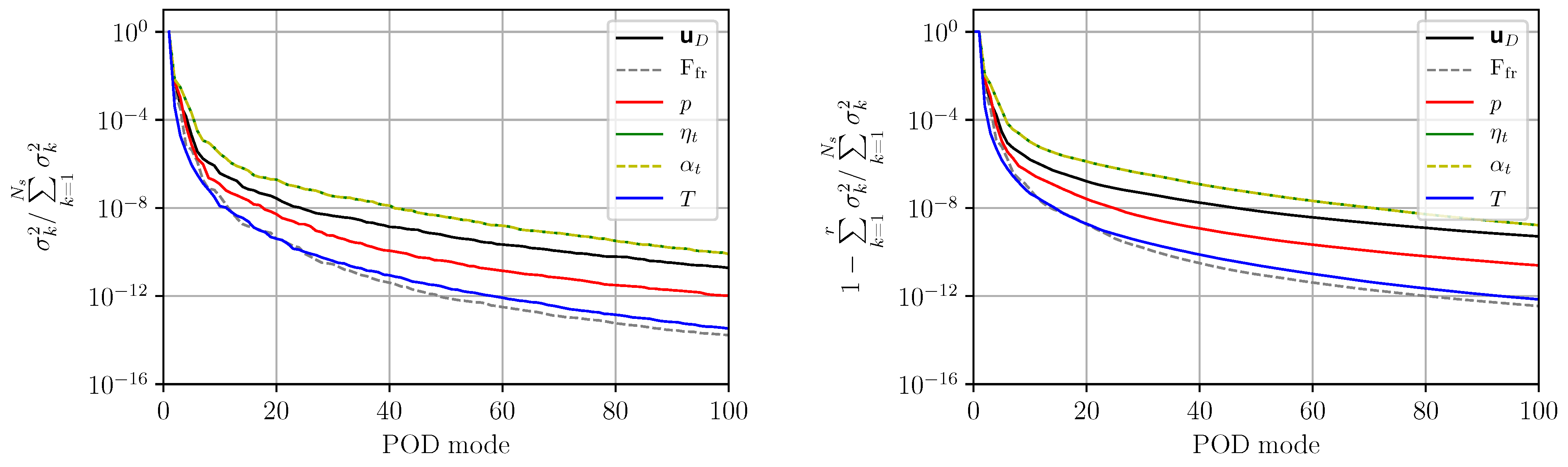
2.2. Training Reduced-Order Models

The training of the ROMs continues with the collection of information about the parameter- and time-dependent solution manifold. This is carried out using the method of snapshots [11], in which the FOM is exercised to obtain N s snapshots of the system at different time instances and/or model parameter values. In this work, we assume that N μ different parameter samples are used and snapshots are saved at N τ different time instances, yielding a total number of N s = N μ × N τ snapshots for a parametric transient and N s = N μ for parametric steady-state runs.
For FOMs built using FVM, a snapshot is a vector of length N or 3 N (assuming three spatial dimensions) for scalar and vector fields, respectively. The snapshots for field X = { u D , p , T , F f r , z , η t , α t } are stored in corresponding snapshot matrices denoted by R X :
R X = [ X ( t 1 , μ 1 ) , X ( t 2 , μ 1 ) , . . . , X ( t N T τ 1 , μ N μ ) , X ( t N τ , μ N μ ) ] ,
where we see that, in addition to the snapshots of the solution fields, we capture the eddy viscosity ( η t ), eddy diffusivity ( α t ), and the flow resistance force in porous medium zone z = 1 , . . . , N z as well. The importance of saving these snapshots is discussed later in detail.
Next, we introduce the reduced-basis approximations for the fields of interest. We assumed that the time- and parameter-dependent solution vectors live in a considerably smaller subspace of R N . In other words, we assume that the fields of interest can be approximated as the linear combination of only a few, space-dependent global basis vectors ( ψ X ). This also means that the summation coefficients ( c X = c X ( t , μ ) ) in the linear combination are responsible for capturing the time- and parameter-dependence of the approximate solution. For the Darcy velocity and corrected pressure fields, this can be expressed as follows:
u D u ˜ D = i = 1 r u D ψ i u D c i u D = Ψ u D c u D , and p p ˜ = i = 1 r p ψ i p c i p = Ψ p c p .
Instead of the real velocity, we approximate the Darcy velocity ( u D ). The reason for this is that u D is smooth in space and, therefore, can be better approximated using global basis functions. Similarly to the velocity and pressure, the temperature field can be approximated as:
T T ˜ = i = 1 r T ψ i T c i T = Ψ T c T .
Moreover, for simulations involving turbulence, the turbulent eddy viscosity ( η t ) and the turbulent diffusivity ( α t ) are also approximated as follows:
η t η ˜ t = i = 1 r η t ψ i η t c i η t = Ψ η t c η t , and α t α ˜ t = i = 1 r α t ψ i α t c i α t = Ψ α t c α t ,
Lastly, a reduced-basis approximate is constructed for the flow resistance in porous medium zone z as:
F f r , z F ˜ f r , z = i = 1 r F f r , z ψ i F f r , z c i F f r , z = Ψ F f r , z c F f r , z .
In this work, the spatial basis vectors of the fields of interest are obtained via Proper Orthogonal Decomposition (POD) [10,13,44] applied to the snapshots. This involves the discovery of a reduced set of orthonormal basis functions that span a subspace of fixed rank that is closest to the snapshots in a global L 2 sense. For field X, this optimization problem can be expressed as follows:
span { ψ i X } = arg min span { ψ i X } s = 1 N s X s i = 1 r X ψ i X , X s Ω ψ i X L 2 2 , with ψ i X , ψ j X Ω = δ i , j ,
where a , b Ω denotes the inner product between fields a and b. For FVM, this equivalent to following matrix product a T M Ω b where M Ω is a mass matrix containing the volumes of the mesh cells on the diagonal. In practice, the basis functions of the reduced subspaces can be obtained using a constrained Singular Value Decomposition (SVD) [45] of the snapshot matrix:
R X = Ψ X Σ X Q X , T , with Ψ X M Ω Ψ X , T = I .
Once the SVD of R X is computed, the first r X columns of the left singular vector matrix Ψ X can be used as the basis vectors for the reduced-basis approximation. The selected basis vectors are often referred to as POD modes, and the two expressions are used interchangeably in this work. Moreover, r X is the rank of the subspace and can take a maximum value of N s . In the examples presented in Section 3, an energy truncation strategy is used to determine the actual value for r X . This utilizes the singular values ( σ i X , i = 1 , . . . , N s ) on the diagonal of Σ X :
r X = arg min 1 r N s k = 1 r X σ X , 2 k = 1 N s σ k X , 2 > 1 τ ,
where τ is a truncation threshold. In general, as the truncation value decreases (i.e., as 1 τ 1 ), more basis functions are used to build the reduced subspaces. The basis functions for X = { u D , p , T , F f r , z , η t , α t } are constructed using this approach.
Once the basis functions are computed, the reduced-basis approximations in Equations (12)–(15) are plugged back into Equations (1), (2) and (9). Following this, the equations are projected using the basis functions of the corresponding solution variable (Galerkin projection). This results in the following reduced equation system for the linear momentum and mass conservation equations:
ρ G c u D = 0 , ρ M c ˙ u D + ρ c u D , T C ¯ ¯ c u D c η , T T ¯ ¯ c u D η D c u D + P c p
z = 1 N z | F p , z | S p , z S f r , z c z F f r ρ β t h A c T = 0 ,
where the elements of the low order vectors, matrices, and higher-order tensors are computed as:
M i , j = ψ i u D , ψ j u D Ω C ¯ ¯ i , j , k = ψ j u D , 1 γ · ψ i u D ψ k u D Ω D i , j = ψ i u D , · ψ j u D + ( ψ j u D ) T Ω P i , j = ψ i u D , γ ψ j p Ω S p , z , i = ψ i u D , γ δ z ( r ) F p , z | F p , z | Ω G i , j = ψ i p , · ψ j u D Ω , T ¯ ¯ i , j , k = ψ j u D , · ψ i η t ψ k u D + ( ψ k u D ) T Ω S f r , z , i , j = ψ i u D , δ z ( r ) ψ j F f r , z Ω A i , j = ψ i u D , g · r ψ j T Ω
where δ z ( r ) is a selection function, which returns 1 if r is in porous medium zone z and 0 otherwise. In this scenario, the expansion coefficients of the temperature ( c T ) are considered to be fixed. To be able to solve system (19) and (20) for the expansion coefficients of the velocity and pressure ( c u D , c p ), however, three additional issues need to be addressed:
  • In this form, the two-equation ROM is not stable since the Ladyzhenskaya–Babuska–Brezzi (LBB) condition [46] is not necessarily satisfied. For this reason, an approximate supremizer stabilization [14,18] is used. This entails the generation of supremizer snapshots using the pressure snapshots by solving the following problem:
    Δ s i = p i , r Ω , i = 1 , . . . , N s
    s i = 0 , r Γ .
    The supremizer snapshots are collected in a snapshot matrix ( R s ) and the corresponding Ψ s basis functions are generated using the constrained SVD. Then, the velocity reduced subspace is augmented by these basis functions. In practice, this means that the supremizer basis vectors are appended to the velocity basis matrix: Ψ u D [ Ψ u D Ψ s ] .
  • The coefficients of the eddy viscosity and diffusivity are still unknown. The computation of these coefficients from reduced forms of eddy-viscosity models is not widely utilized by the fluid dynamics ROM community; therefore, a non-intrusive, data-based approach—Radial Basis Function (RBF) interpolation—was chosen in this work. The effectiveness of this method has been demonstrated in [19,20,21,34]. This approach interpolates coefficients c η t and c α t within the parameter space and time using the snapshots as anchor nodes.
  • The coefficients of the flow resistances are still unknown. In this work, the Discrete Empirical Interpolation Method (DEIM) [47] is used for the determination of these models based on the coefficients of the Darcy velocity. This can be expressed as:
    c z F f r = P z T Ψ F f r , z 1 P z T F f r ( Ψ u D c u D ) ,
    where P z T is a matrix that selects r F f r , z rows when applied to a vector. In this work, P z T was constructed using the algorithm published in [47]. This method ensures that the evaluation of the flow resistance at reduced-order level is computationally efficient.
As a next step, the porous medium enthalpy equation is reduced with the same process. The reduced-basis approximates are plugged into Equation (9), and the resulting expression is projected using the basis functions of the temperature:
ρ c p M γ c ˙ T + ρ c p c u d , T A ¯ ¯ c T k l K l c T c α t , T c p K ¯ ¯ t c T = z = 1 N z h z A V z M z c T + z = 1 N z h z A V z T ext s h z + Q r ,
where the elements of the reduced operators and source terms can be expressed as:
M γ i , j = ψ i T , γ ψ j T Ω , A ¯ ¯ i , j , k = ψ i T , · ψ k u D ψ j T Ω ,
K l i , j = ψ i T , · γ ψ j T Ω , K ¯ ¯ t i , j , k = ψ i T , · γ ψ k α t ψ j T Ω ,
M z i , j = ψ i T , δ z ( r ) ψ j T Ω , s h z i = ψ i T δ z ( r ) Ω ,
Q r i = ψ i T , Q Ω .

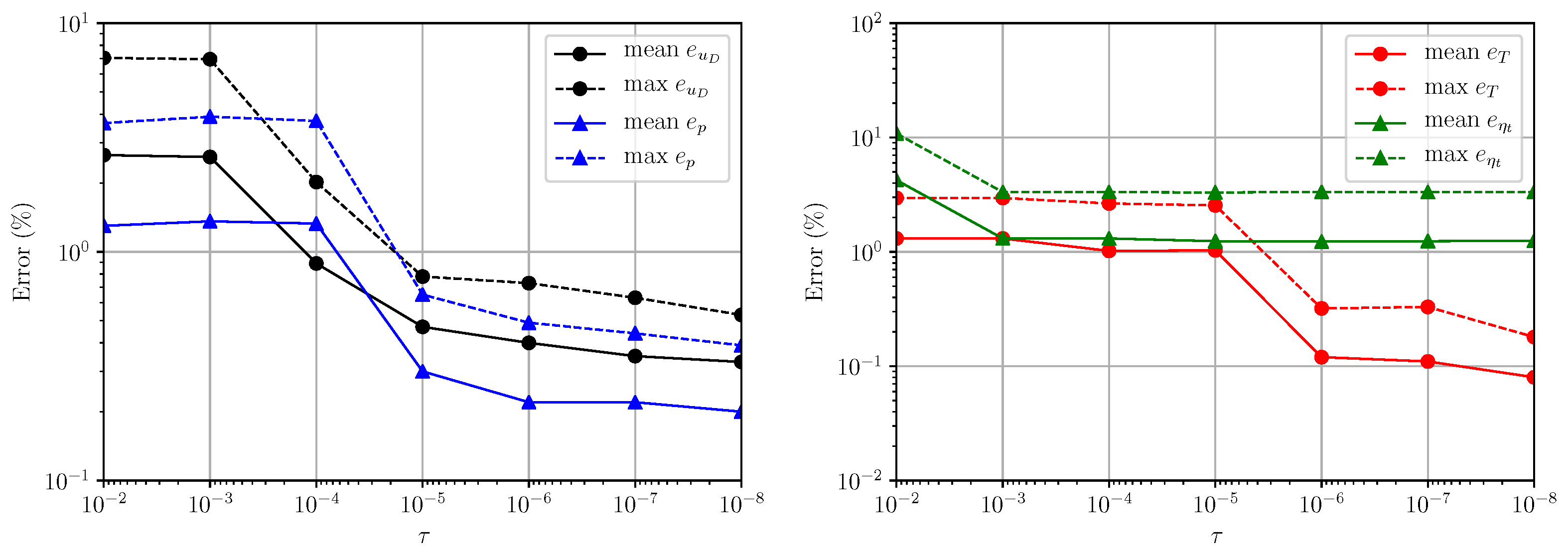
2.3. Evaluating Reduced-Order Models

Once the training phase of the ROM is concluded, we enter the online/evaluation phase. This phase starts with the assembly of the ROM using a new parameter sample ( μ ) where the quantity of interest needs to be evaluated. This is computationally cheap if the reduced-operators are affine in the model parameters and time, which allow us to express the reduced-order operators as a sum of products of space-dependent operators ( A i ) and solution-, parameter-, and time-dependent scalar functions ( f i ( c X , t ; μ ) ) as:
A ( c X , t ; μ ) = i A i f i ( c X , t ; μ ) .
In this scenario, the assembly of the reduced-order model simplifies into the summation and scalar multiplication of small, precomputed matrices and vectors from the training phase. By looking at Equations (19), (20) and (24), we conclude that the ROMs are affine in the following parameters: the density ( ρ ), the magnitude of the pumping power in the porous medium zones ( | F p , z | ), the thermal expansion coefficient ( β t h ), the molecular dynamic viscosity ( η ), the specific heat ( c p ), the thermal conductivity ( k l ), the heat transfer coefficient ( h z ), and the external coolant temperature ( T ext ) in the heat exchangers. Furthermore, through the utilization of DEIM, the problem becomes affine in the parameters of the flow resistance function as well.
Since the ranks of the selected subspaces are typically much lower than the size of the original, full-order system ( r X N ), the assembly of the ROM is computationally cheap. This process is followed by the solution of the ROM for the expansion coefficients. In this work, an implicit Euler discretization is used for time-dependent problems, while the nonlinearities are resolved using a nested fixed-point iteration between the fluid ROM and enthalpy ROM. Once the expansion coefficients are obtained, the reduced-basis approximates can be reconstructed and the quantities of interest (point values, averages, etc.) can be evaluated at the new parameter sample ( Q o I ( μ ) ).

3. Results

We demonstrate the applicability of the developed ROM to parametric steady-state and transient problems in the Molten Salt Fast Reactor (MSFR) [33]. For this, a 2D axisymmetric model is employed. The MSFR is a liquid-fuel nuclear reactor in which the fissile material is dissolved in a molten salt that is circulated in a loop. Heat (3 G W t h ) is generated by the nuclear fission reactions and is predominantly deposited in the liquid fuel. Figure 2 shows the geometry and mesh used for the simulations together with the distribution of the power deposition. The mesh was adopted from [34] and contains 16,140 cells.
For every scenario in this work, this distribution is considered to be fixed. The red and blue regions in the mesh denote porous medium zones, while clean fluid is shown in green. The molten salt fluid enters the core cavity through the core inlet, warms up, and leaves through the core outlet. The molten salt then cools off in the heat exchanger. This example has been specifically chosen to showcase how a system with both clean fluid and prorous medium zones can be treated with the developed ROM.
Even though we use a nuclear reactor as an example, the developed ROMs can be used for chemical reactors and other industrial loops involving heat transfer. Both steady-state and transient examples assume a turbulent flow regime, with approximate Reynolds numbers in the [ 6.72 × 10 5 , 1.23 × 10 6 ] interval within the core cavity. The default values of the thermophysical parameters of the fluid were determined using the help of [48] and are summarized in Table 1.
As already mentioned, the pump and the heat exchanger can be treated as porous medium zones. In this work, the pump is treated as a volumetric momentum source with the assumptions that the fluid entirely occupies the volume ( γ = 1 ), and the force exerted by the pump is homogenized in the region with a 100 k N m 3 default value. This is justified by the lack of data on the friction factors and structure of the pump in the MSFR design. The heat exchanger, on the other hand, has been treated as a porous medium with default parameters listed in Table 2.
These parameters are considered to be approximate values, since no specific design has been chosen for the MSFR yet. The parameters describing the flow resistance have been chosen using the Blasius correlation in [49] (assuming a tubular heat exchanger) with slightly increasing A f to obtain a realistic pressure drop in the porous medium zone.
The first numerical example considers a steady-state scenario of the MSFR with several uncertain parameters. As the second case, a transient scenario is analyzed. The transient starts from a steady-state, which is obtained using the default parameters from Table 1 and Table 2. At t = 2 s, a flow coastdown is simulated by linearly ramping down the pumping force from 100 k N m 3 to 20 k N m 3 in Δ t ramp . Figure 3 showcases this transience with Δ t ramp = 8 s.
The problem at hand was discretized in space using corrected linear gradient estimators for the diffusion terms (second order) and a vanLeer [50] scheme for the advection term in the fluid-dynamics equations (also second order). The advection term in the enthalpy equation was discretized using a first order upwind scheme. In terms of time discretization of transient scenarios, both the FOM and the ROM applied a backward Euler scheme.

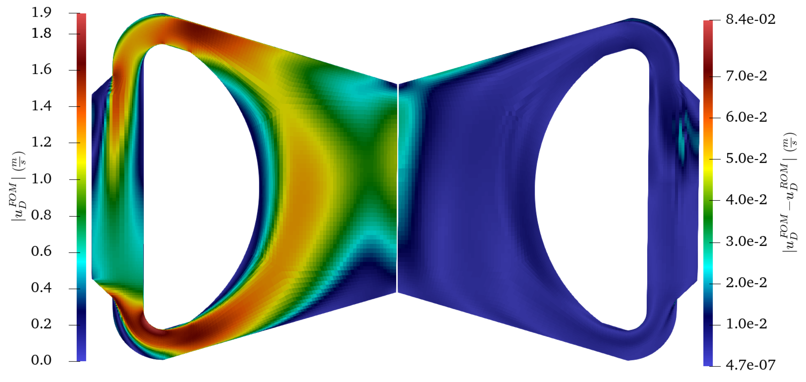
3.1. Reduced-Order Models for Steady-State Problems

First, the applicability of the developed ROM to steady-state scenarios was assessed. For this, five parameters were assumed to be uncertain. The list of these parameters together with the assumed probability distributions is presented in Table 3. In this context, U ( a , b ) is a uniform distribution in the [a,b] interval.
The generation of the ROM for the parametric steady-state simulations starts with collecting snapshots of the fields of interest. Altogether, N s = 40 snapshots were generated by sampling parameter vector μ = [ | F p | , T ext , h , β t h , Pr ] T using Latin Hypercube Sampling (LHS), executing the FOM using the generated samples, and saving the given fields into snapshot matrices. The number of training samples was determined considering the number of uncertain parameters, the available time/computational resources, and resolution constrains for the RBF interpolation of the turbulent eddy viscosity/diffusivity coefficients.
Then, the supremizer snapshots were obtained by solving Equation (22). Following this, the basis functions of the reduced subspaces were extracted from the snapshots using a constrained SVD. The first 3 POD modes of the velocity, pressure and temperature are presented in Appendix A. The decay in the squares of the singular values of the snapshot matrices is presented in Figure 4.
Note, the values were normalized by the square sum of the singular values. Furthermore, since the energy truncation limit ( τ ) was employed in this example for the determination of the number of POD modes used for the generation of the ROMs (see Equation (18)), the truncated energy per POD mode is showcased in Figure 4 as well. Overall, we see a rapid decay in the squared singular values, indicating that the solution exhibits a low-dimensional behavior.
Then, numerous ROMs were prepared with different numbers of basis functions. The number of basis functions for the fields of interest was determined using Equation (18), with two exceptions. The number of modes for the pressure and supremizer fields was determined in a slightly different manner since the inclusion of too many supremizer modes may decrease the accuracy of the ROM. In this work, we used the same number of pressure and supremizer modes. Once the number of POD modes for every other field was chosen using the truncation limit, we performed a one-dimensional optimization to select the number of pressure/supremizer modes, which yielded the highest average accuracy in velocity over the test set.
Furthermore, due to the limited number of snapshots and the relatively high-dimensional parameter space, the RBF interpolation for coefficients of the eddy viscosity and diffusivity is restricted to the pumping-force alone, simplifying it to a one-dimensional problem. This can be justified by the fact that the other parameters influence the fluid dynamics equations through the buoyancy effect, which is significantly lower than the effect of changing the pumping force itself.
As a next step, a validation set was assembled by drawing N val = 20 new parameter samples using LHS. The size of the test set was determined to be half of that of the training set due to the FOM being relatively expensive to solve, limiting the available data. These samples were used to test (validate) the ROMs with respect to the FOM. The parameter vectors in the validation set were plugged back into the FOM, and the different ROMs and the corresponding FOM solution fields were compared to the reconstructed reduced-basis approximates from the ROMs. We chose the relative L 2 error for an indicator:
e X = | | X F O M X R O M | | L 2 | | X F O M | | L 2 ,
where X = { u D , p , T , η t , α t } . The average and maximum errors over the validation set as functions of the truncation parameter τ are presented in Figure 5. We see a considerable decrease in the error as we decrease the truncation parameter. The error in the eddy viscosity went to saturation. This was caused by the fact that the error in the RBF interpolation became more dominant compared to the approximation error beyond τ = 10 4 . The behavior of α t was exactly the same as η t since the two fields (in this work) differ only by a constant factor (turbulent Prantl number, Pr t ).
The ROM built with τ = 10 8 was selected for further investigation. The number of modes used for the fields of interest together with the error statistics over the validation set are presented in Table 4. Moreover, the selected ROM utilized seven modes for the flow resistance in the heat exchanger during the DEIM process. It is visible that, with the exception of η t / α t , the maximum relative L 2 error was below 0.53%, which is considered to be adequate.
Since the relative L 2 error is an integrated quantity, we present the distribution of the local errors of the velocity and temperature fields at the test sample, which exhibited the highest errors in terms of the velocity. Figure 6 shows the FOM solution (to the left) and the absolute error between the FOM and the ROM (to the right). It is visible that the maximum error was attained at the outlet of the heat exchanger within the corner element in the mesh. At this point, the relative error was close to 5% locally. In other parts of the reactor, we see considerably lower relative errors. Note that the error appears to be especially low in the heat exchanger meaning that the DEIM process seems to be efficient for the approximation of the flow resistance.
Figure 7 presents the temperature solution of the FOM (left) together with the absolute error between the FOM and the ROM (right).
We see that the maximum error was attained at the bottom of the core cavity. At this point, the relative error slightly exceeded 1% locally, while, at other parts of the reactor, the error remained significantly lower.
Lastly, we evaluated the computational time savings of using a ROM (built with τ = 10 8 ) instead of the FOM. Obtaining the FOM solutions for a parameter combination took approximately 4000 s on average, while the same was 0.1 s using the ROM. This means that an approximate single-run speedup of 40,000 was achieved.

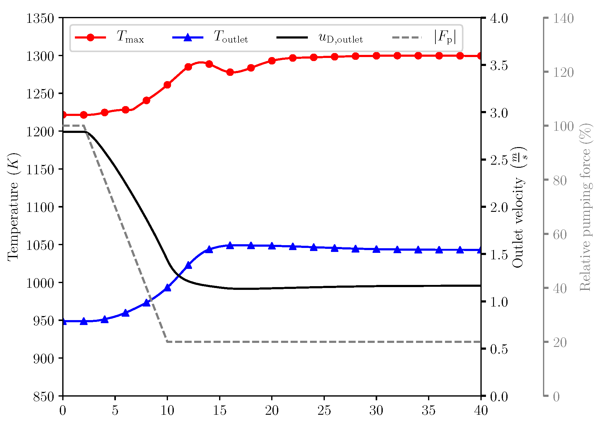
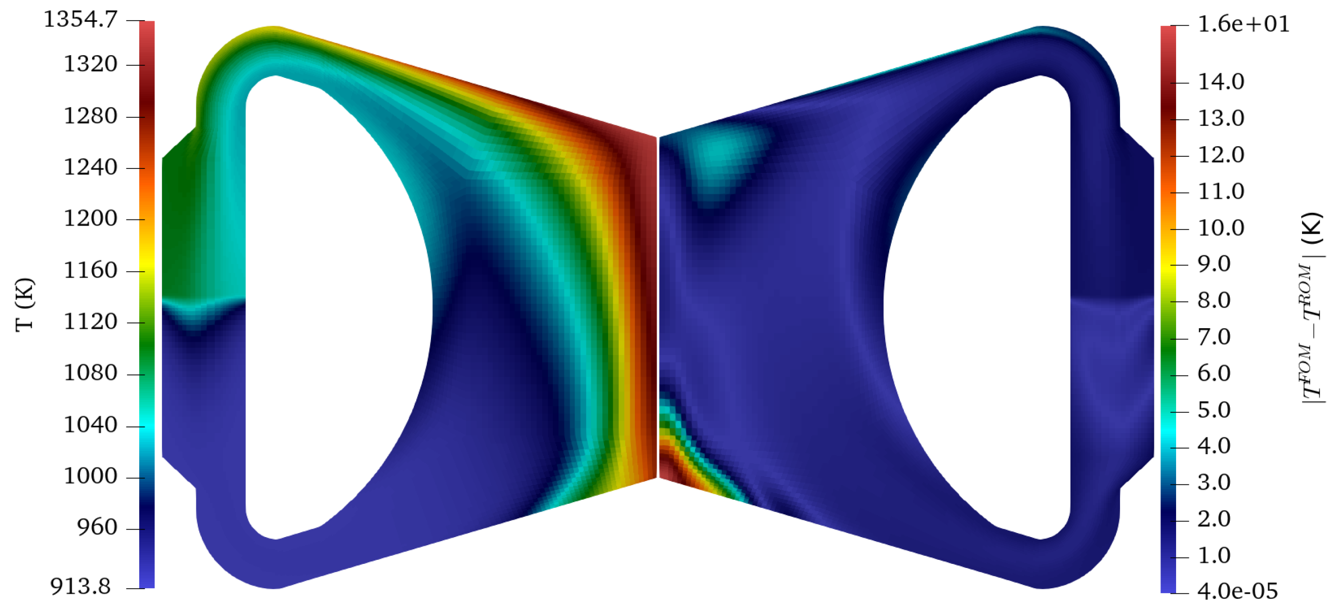
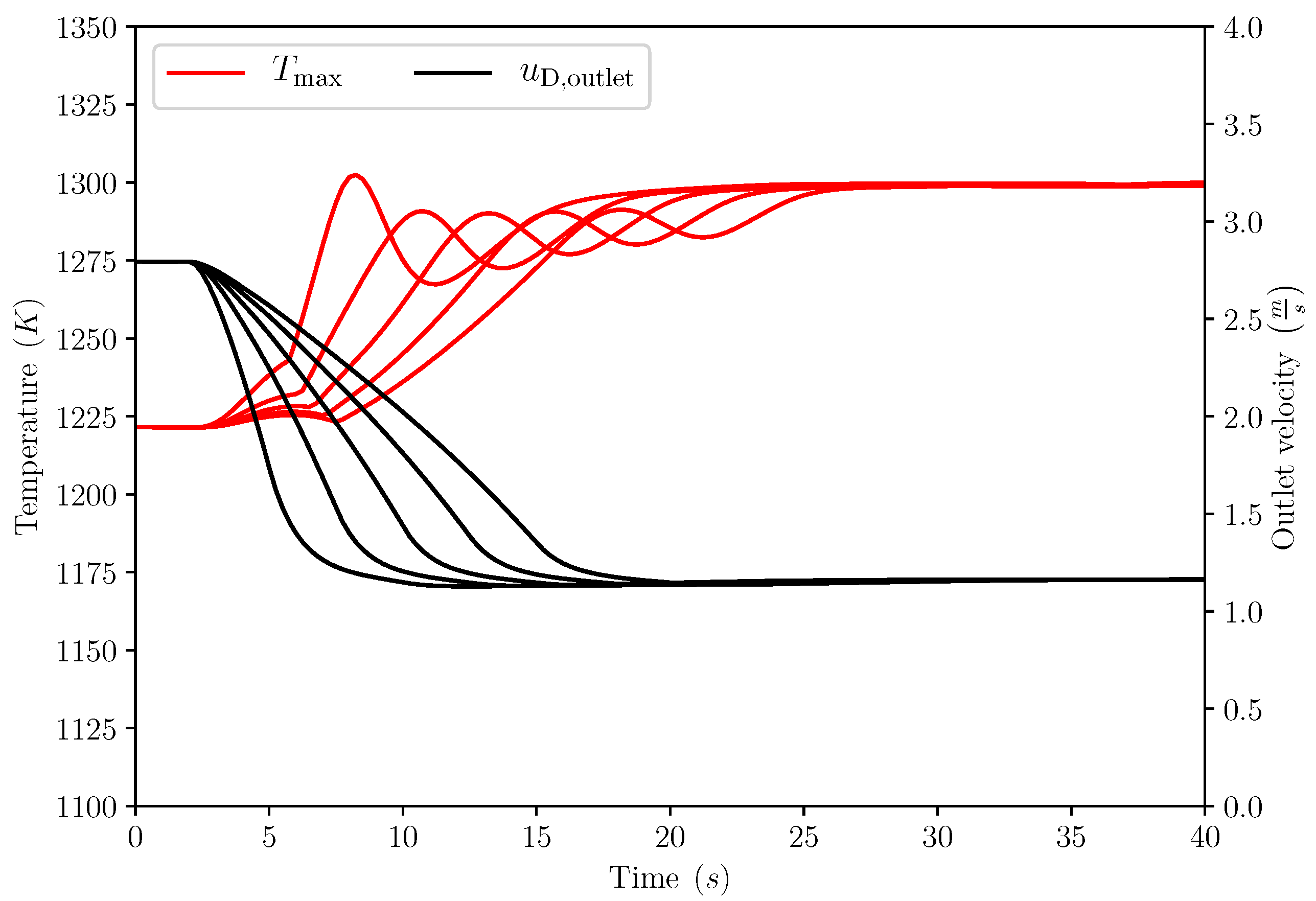
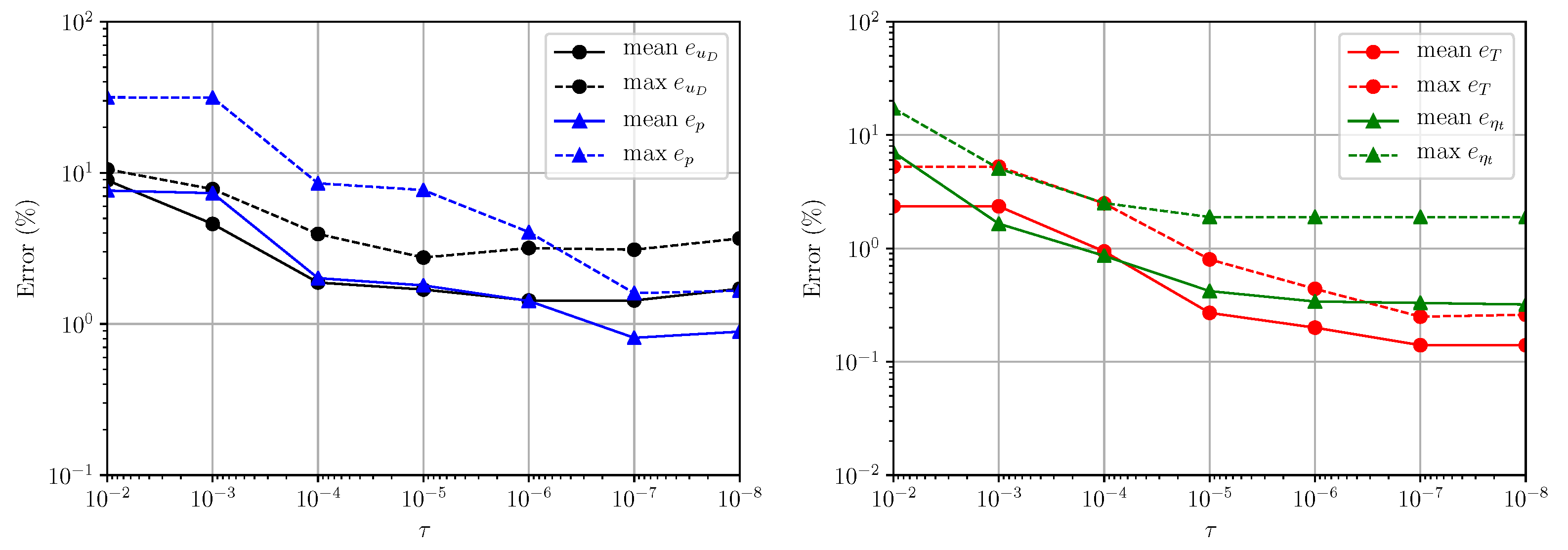
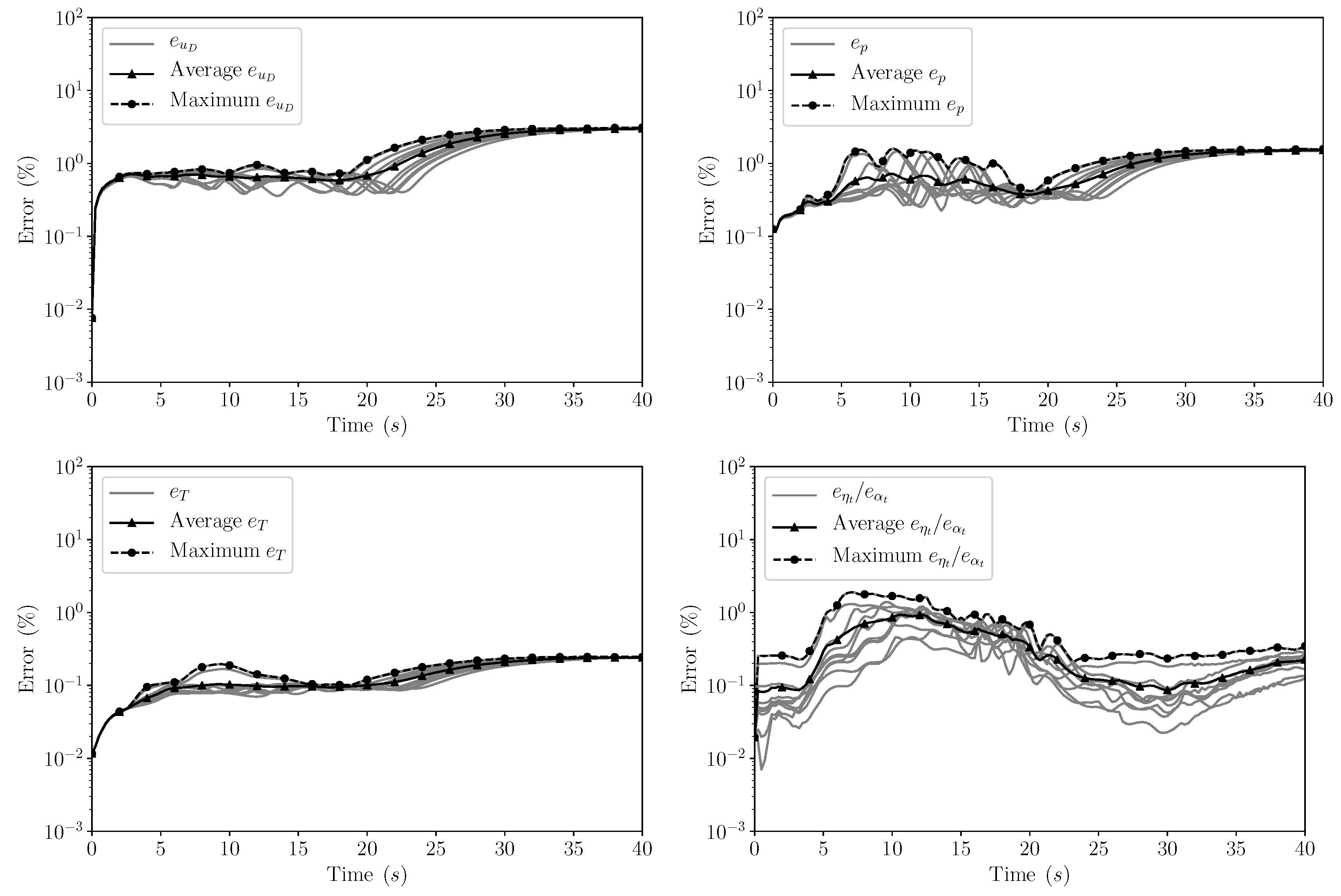
3.2. Reduced-Order Models for Transient Problems

The transient scenario used in this work simulates a pump coastdown from 100% to 20% of the nominal power. The transient is visualized in Figure 3. We consider the time needed to reach the new power level an uncertain parameter with a uniform distribution: Δ t ramp U ( 3 , 13 ) s . The generation of the reduced-order model starts with the collection of snapshots. Altogether, five transients are solved evenly spaced in coastdown times. The number of training samples was chosen to ensure an adequate accuracy in the RBF interpolation of the eddy viscosity/diffusivity coefficients while still considering the relatively expensive solutions of the FOM.
The training scenarios are presented in Figure 8. It is visible that there was an oscillation in the maximum temperature in the system, which depended on the dynamics of the velocity field. We took snapshots of the system every 0.25 s for each scenario meaning that, altogether, 805 snapshots were used to build the reduced subspaces. The decay in the normalized squared singular values and the truncated energy are presented in Figure 9. We see that the singular values decayed much slower compared to the steady-state results. This implies that the time-dependence in the problem introduced considerable spatial variation in the fields of interest.
As a next step, the basis functions of the fields of interest were built using POD. The first 3 POD modes of the velocity, pressure and temperature are presented in Appendix B. The number of basis functions were determined using the strategy already discussed in Section 3.1, which involves the definition of an energy truncation limit ( τ ). Several ROMs were then prepared with different values of τ . These ROMs were tested on 10 additional pump coastdown times that were randomly sampled from the [3, 13] s interval (test set). In must be noted that, in this scenario, the ratio of test samples to training samples is higher because the expected variation of the solutions in time and parameter space is larger compared to the steady-state problem.
The relative L 2 error defined in Equation (30) was evaluated for each solution field over time. The maximum and average errors over the test set and time as function of the energy truncation parameter are presented in Figure 10. We see a decrease in the average error in the 10 2 10 7 interval. Beyond this, the errors slightly increased, which can be explained by the buildup of the errors discussed later in Section 4.
The number of modes together with the average and maximum errors for τ = 10 7 are presented in Table 5. We see that over all the solution fields, times, and test sets, the maximum relative L 2 error was 3.3%, which is adequate for engineering applications. Furthermore, we note that the ROM was capable of the reconstruction of the temperature field with a maximum L 2 error slightly below 0.25%, which is also considered to be accurate.
The number of basis functions used to build this ROM is considerably higher than those presented in the steady-case example. This is the direct consequence of the large spatial variation of the solution fields introduced with the time-dependence.
The time-dependent error curves of the field variables over the test parameter set are presented in Figure 11 for τ = 10 7 . It is visible that, for the velocity, pressure and temperature, the highest relative errors appeared in the new steady-state in many cases. The possible reasons behind these effects are further discussed in Section 4.
Lastly, the savings in computation time were evaluated. The execution of the FOM took approximately 16,000 s on a single core of a processor, while the same was around 310 s for the ROM built using τ = 10 7 . This yielded a moderate speedup factor of 51.6. The relatively slow ROM was the result of one of the shortcomings of the RBF interpolation, namely that the 41 coefficients (for both α t and η t ) need to be interpolated using 805 anchor points at every single time step. Other operations needed for the assembly and solution of the ROM are of considerably lower operation count. Assuming that using 21 POD modes are sufficient for the eddy viscosity/diffusivity (corresponds to τ = 10 6 ), the execution time of the ROM decreased to 170 s on average, which resulted in a speedup factor of 94.1.

4. Discussion

Based on the results presented in Section 3, several observations were made about the performance of POD-RB-ROMs for porous medium flows.
First, the supremizer stabilization method for the ROM was not optimal for the handling of turbulent buoyant flows described using Equations (2) with the corrected pressure. This may be the reason behind the ROMs yielding higher relative errors at the new equilibrium levels in the transient scenarios where the buoyancy forces are considerable compared to the momentum source of the pump. Originally, the supremizer stabilization was derived for steady-state clean laminar fluid flows [14]; therefore, the presence of space-dependent diffusivities, porosity factors, and buoyancy-altered corrected pressure terms may require the modification of the original concept. A possible approach could be the inclusion of these aspects in the supremizer equation in Equation (22).
Second, it is visible that the errors for transient problems may slightly increase if too many POD modes are used (beyond τ = 10 7 ). This can be the result of the utilization of first-order upwind schemes for the treatment of the advection term in the enthalpy equation, which leads to numerical inconsistency between the FOM and the ROM. The reason behind this is that the discretization of the · ( ψ i u D ψ j T ) terms depends on ψ i u D itself, which is not necessarily the same as the discretization used for · ( u D T ) . This effect can be further amplified by the inclusion of supremizer modes, which do not have a physical meaning.
Third, the DEIM-based method for the handling of the interactions between the fluid and the homogenized structure showed promising results. Even though the relative errors in the flow resistances were not evaluated separately, the low errors in the velocity and pressure ROMs indicate that the flow resistances were treated properly.
Fourth, we observed that the adopted RBF interpolation technique had shortcomings for both steady-state and transient problems. In the case of parametric steady-state scenarios, the parameter space may have to be shrunk to obtain adequate accuracy for the interpolation since, in higher parameter spaces, with a limited number of anchor points, the method yielded results with low accuracy. However, neglecting parameter dimensions in the interpolation introduced additional errors as well.
In the case of transient scenarios, the RBF interpolation may considerably slow down the execution of the ROM due to the fact that some transient scenarios may require a large number of POD modes for the eddy viscosity/diffusivity. Coupled with a large number of anchor points in the interpolation, this may yield relatively slow ROMs. A possible improvement on this part may be the utilization of the sparsity in the problem in a sense that the interpolation at a given parameter sample should only evaluate contributions from anchor points that are in its vicinity.

5. Conclusions

A data-driven Reduced-Order Model (ROM) was developed for the incompressible porous medium RANS equations coupled with the porous medium enthalpy equation. The ROMs were generated using an intrusive Proper Orthogonal Decomposition aided Reduced-Basis (POD-RB) technique coupled with the method of snapshots. The process involved the exploration of the parameter- and time-dependent solution manifolds by solving a higher-fidelity model (or Full-Order Model, FOM) and saving the solution fields as snapshots. The information in these snapshots was then compressed using POD into global spatial basis functions, which were then used to approximate the higher-fidelity solution and to project the equations onto reduced subspaces.
This resulted in a considerable reduction in the spatial degrees of freedom, and, consequently, in the execution time as well. The developed ROM utilized a supremizer stabilization for the reduced porous medium fluid dynamics equations and a Radial Basis Function (RBF) interpolation for the handling of the turbulent viscosity/diffusivity at reduced-order level. The flow resistance exerted by the homogenized structural elements in the flow was treated using the Discrete Empirical Interpolation Method (DEIM).
To the best of the authors’ knowledge, the developed ROM is a novel contribution to the fluid dynamics ROM literature. Moreover, this method can be considered as an alternative for approaches where fluid dynamics POD-RB-ROMs are used for large volumes of clean fluids and thermal-hydraulics system codes for other elements in the loop [32].
The ROM has been tested using a 2D axisymmetric model of the Molten Salt Fast Reactor (MSFR), which contains clean fluid and porous medium zones in the same thermal-hydraulic loop. The results indicate that the developed ROMs can be used to accurately emulate parametric steady-state and transient problems. The relative L 2 errors of the POD-RB-ROMs were always below 3.3%, which is considered adequate, especially for engineering applications. While the achieved speedup is on the order of 10,000 for the steady-state scenarios, it decreases to 51–94 for transient cases. This can be explained by the shortcomings of the RBF interpolation.
Overall, from an engineering perspective, the developed ROMs yielded accurate solutions. Compared to the accuracy requirements for steady-state simulations with thermal-hydraulics system codes in the nuclear industry, the reduced-order model errors were well below the recommended limits [51].

Author Contributions

Conceptualization, P.G. and J.C.R.; Methodology, P.G. and M.E.T.; Software, P.G., M.E.T.; Validation, P.G.; Formal analysis, P.G.; Investigation, P.G.; Resources, J.C.R. and C.F.; Data curation, P.G.; Writing—original draft preparation, P.G.; Writing—review and editing, P.G., M.E.T., J.C.R. and C.F.; Visualization, P.G.; Supervision, J.C.R., M.E.T. and C.F.; Project administration, J.C.R.; Funding acquisition, J.C.R. and C.F. All authors have read and agreed to the published version of the manuscript.

Funding

This research was carried out with funding received from the United States Department of Energy, Office of Nuclear Energy’s Nuclear Energy University Program grant No. DE-NE0008651.

Institutional Review Board Statement

Not applicable.

Informed Consent Statement

Not applicable.

Data Availability Statement

Not applicable.

Conflicts of Interest

The authors declare no conflict of interest.

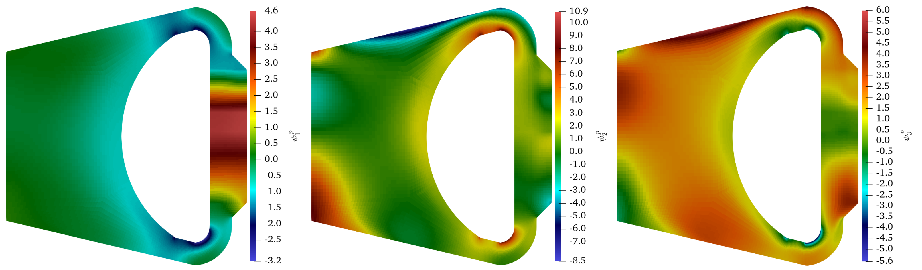
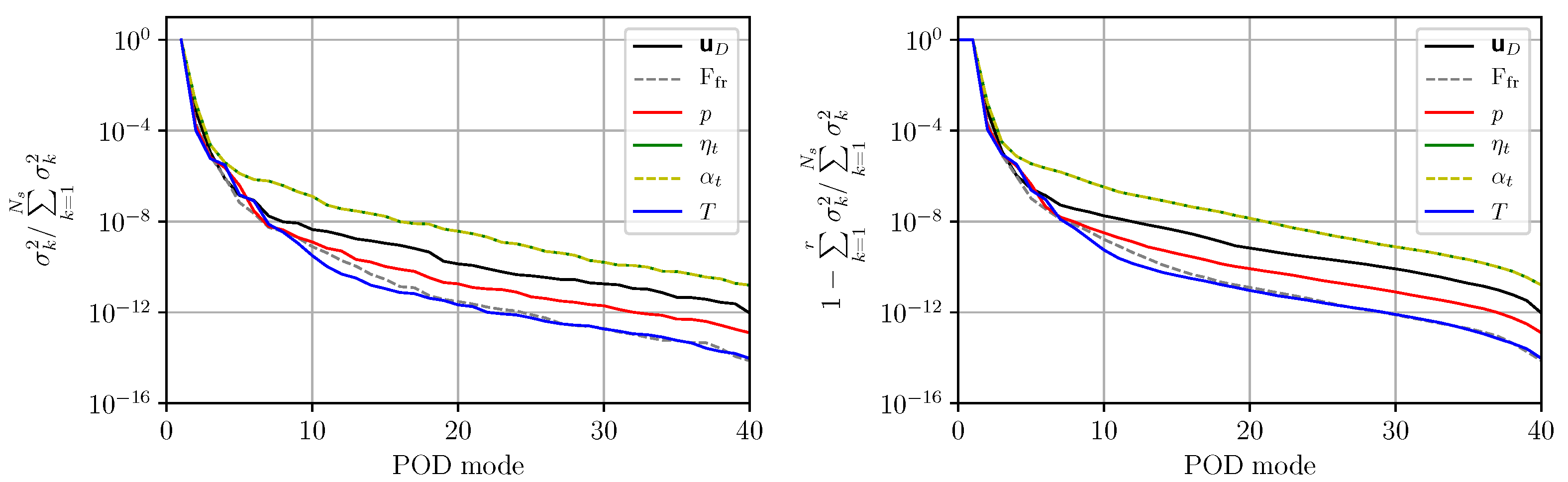
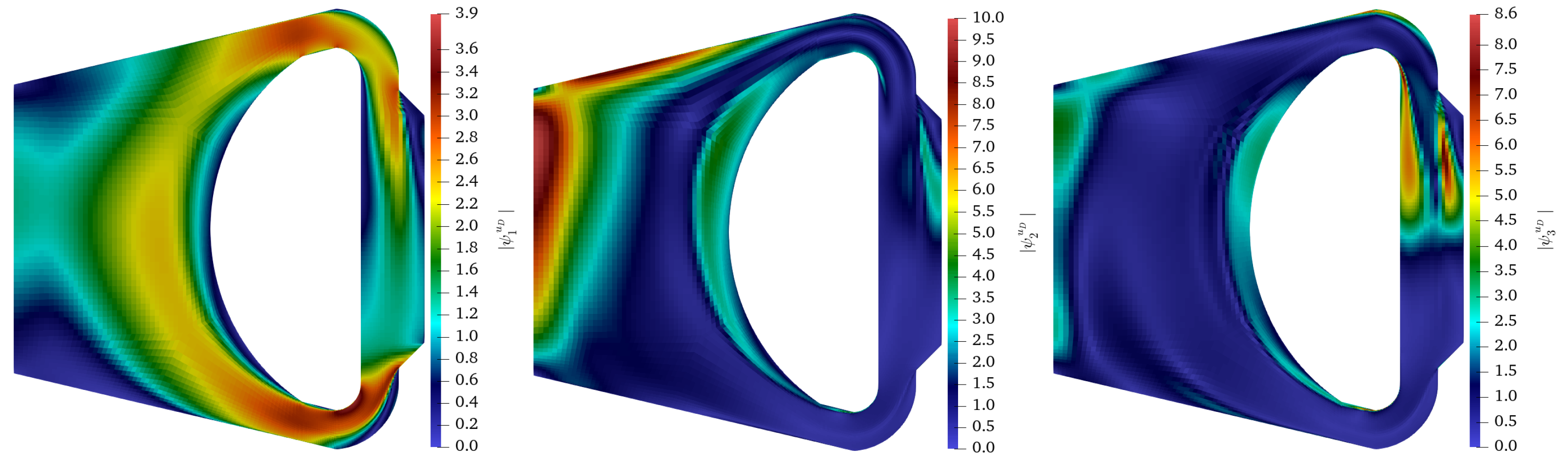
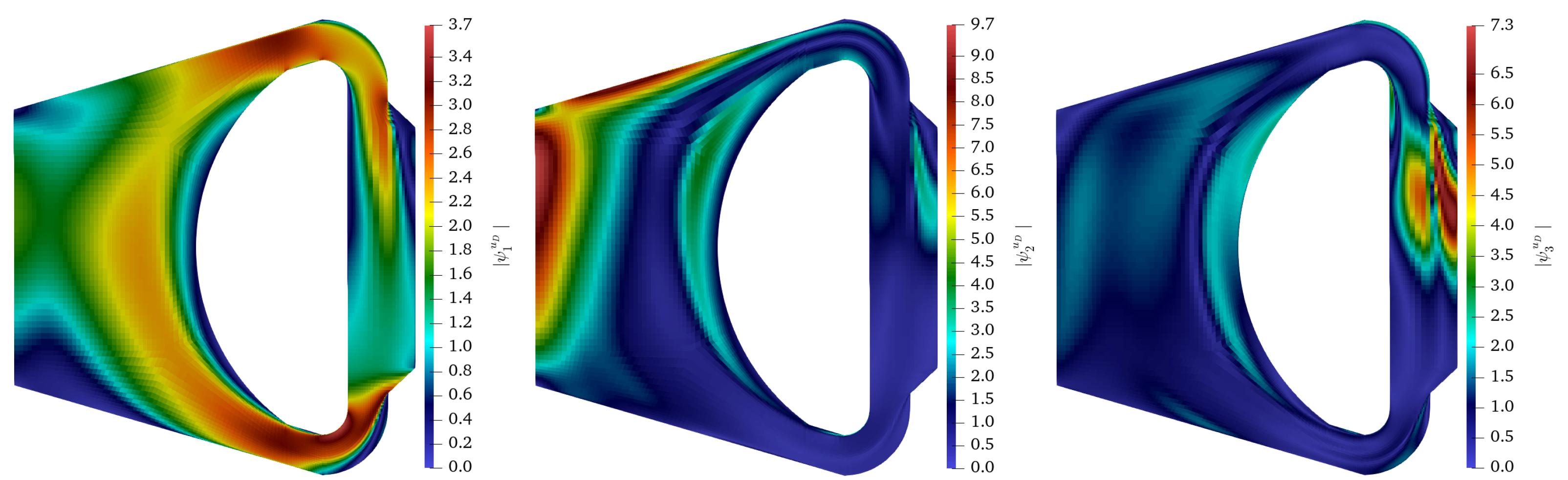
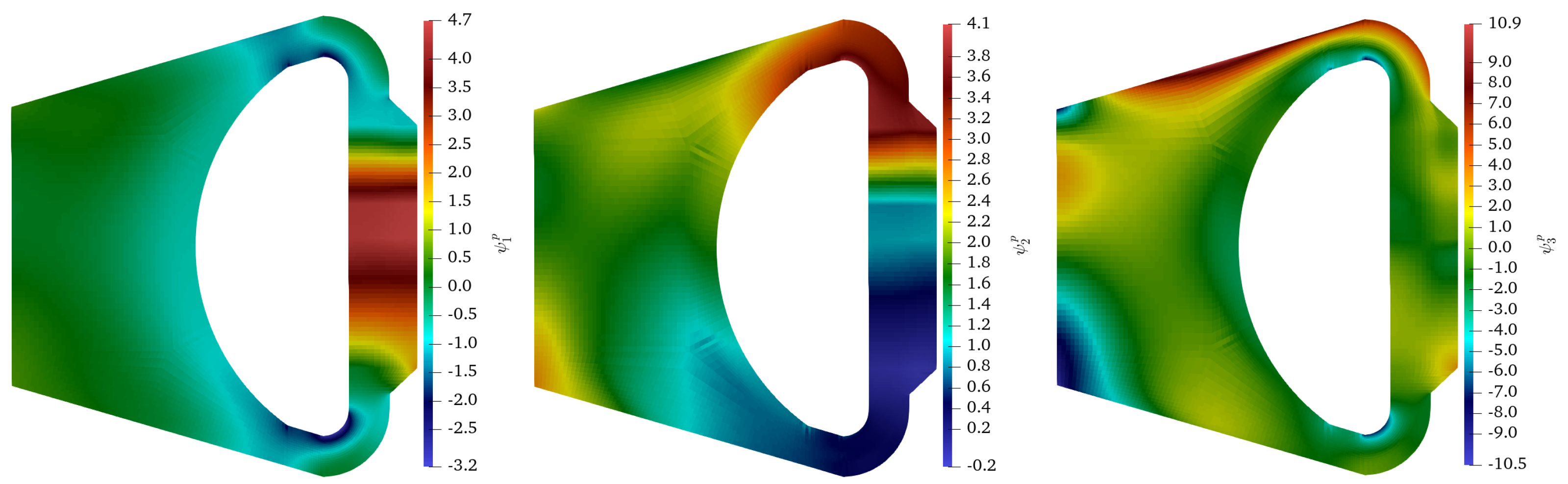
Appendix A. POD Modes of the Steady-State Problem

Figure A1. First three (left to right) POD modes of u D in the case of the steady-state numerical example.
Fluids 06 00266 g0a1
Figure A2. First three (left to right) POD modes of p in the case of the steady-state numerical example.
Fluids 06 00266 g0a2
Figure A3. First three (left to right) POD modes of T in the case of the steady-state numerical example.
Fluids 06 00266 g0a3

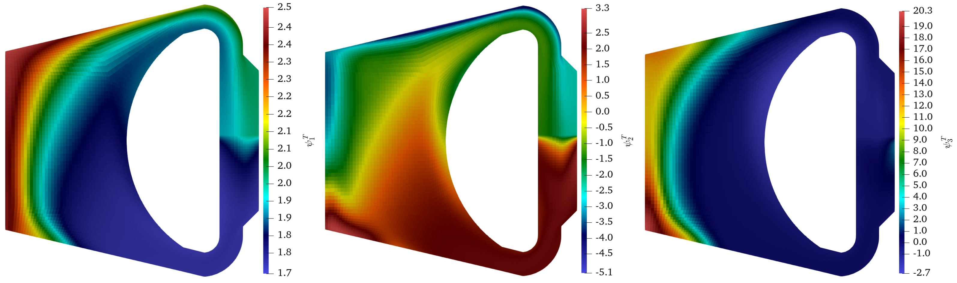
Appendix B. POD Modes of the Transient Problem

Figure A4. First three (left to right) POD modes of u D in the case of the transient numerical example.
Fluids 06 00266 g0a4
Figure A5. First three (left to right) POD modes of p in the case of the transient numerical example.
Fluids 06 00266 g0a5
Figure A6. First three (left to right) POD modes of T in the case of the transient numerical example.
Fluids 06 00266 g0a6

References

  1. Hu, R. A fully-implicit high-order system thermal-hydraulics model for advanced non-LWR safety analyses. Ann. Nucl. Energy 2017, 101, 174–181. [Google Scholar] [CrossRef] [Green Version]
  2. Hu, R.; Zou, L.; Hu, G.; Nunez, D.; Mui, T.; Fei, T. SAM Theory Manual; Technical Report; Argonne National Lab. (ANL): Argonne, IL, USA, 2021.
  3. Berry, R.A.; Peterson, J.W.; Zhang, H.; Martineau, R.C.; Zhao, H.; Zou, L.; Andrs, D.; Hansel, J. Relap-7 Theory Manual; Technical Report; Idaho National Lab. (INL): Idaho Falls, ID, USA, 2018.
  4. Plit, H.; Kontio, H.; Kantee, H.; Tuomisto, H. LBLOCA Analyses with APROS to Improve Safety and Performance of Loviisa NPP. In Proceedings of the OECD-CSNI workshop on Advanced Thermal-Hydraulic and Neutronic Codes, Barcelona, Spain, 10–13 April 2000. [Google Scholar]
  5. Costa, A.L.; Reis, P.A.L.; Pereira, C.; Veloso, M.A.F.; Mesquita, A.Z.; Soares, H.V. Thermal hydraulic analysis of the IPR-R1 TRIGA research reactor using a RELAP5 model. Nucl. Eng. Des. 2010, 240, 1487–1494. [Google Scholar] [CrossRef]
  6. Wu, P.; Gou, J.; Shan, J.; Jiang, Y.; Yang, J.; Zhang, B. Safety analysis code SCTRAN development for SCWR and its application to CGNPC SCWR. Ann. Nucl. Energy 2013, 56, 122–135. [Google Scholar] [CrossRef]
  7. Fiorina, C.; Clifford, I.; Aufiero, M.; Mikityuk, K. GeN-Foam: A novel OpenFOAM® based multi-physics solver for 2D/3D transient analysis of nuclear reactors. Nucl. Eng. Des. 2015, 294, 24–37. [Google Scholar] [CrossRef]
  8. Vafai, K. Handbook of Porous Media; CRC Press: Boca Raton, FL, USA, 2015. [Google Scholar]
  9. Clifford, I.D. A Hybrid Coarse and Fine Mesh Solution Method for Prismatic High Temperature Gas-Cooled Reactor Thermal-Fluid Analysis. Ph.D. Thesis, Pennsylvania State University, State College, PA, USA, 2013. [Google Scholar]
  10. Pearson, K. LIII. On lines and planes of closest fit to systems of points in space. Lond. Edinb. Dublin Philos. Mag. J. Sci. 1901, 2, 559–572. [Google Scholar] [CrossRef] [Green Version]
  11. Sirovich, L. Turbulence and the dynamics of coherent structures. III. Dynamics and scaling. Q. Appl. Math. 1987, 45, 583–590. [Google Scholar] [CrossRef] [Green Version]
  12. Hilberg, D.; Lazik, W.; Fiedler, H.E. The Application of Classical POD and Snapshot POD in a Turbulent Shear Layer with Periodic Structures. Appl. Sci. Res. 1994, 53, 283–290. [Google Scholar] [CrossRef]
  13. Pinnau, R. Model reduction via proper orthogonal decomposition. In Model Order Reduction: Theory, Research Aspects and Applications; Springer: Berlin/Heidelberg, Germany, 2008; pp. 95–109. [Google Scholar]
  14. Ballarin, F.; Manzoni, A.; Quarteroni, A.; Rozza, G. Supremizer stabilization of POD–Galerkin approximation of parametrized steady incompressible Navier–Stokes equations. Int. J. Numer. Methods Eng. 2015, 102, 1136–1161. [Google Scholar] [CrossRef]
  15. Luo, Z.; Chen, J.; Navon, I.; Yang, X. Mixed finite element formulation and error estimates based on proper orthogonal decomposition for the nonstationary Navier—Stokes equations. SIAM J. Numer. Anal. 2009, 47, 1–19. [Google Scholar] [CrossRef] [Green Version]
  16. Tano, M.; German, P.; Ragusa, J. Evaluation of pressure reconstruction techniques for Model Order Reduction in incompressible convective heat transfer. Therm. Sci. Eng. Prog. 2021, 23, 100841. [Google Scholar] [CrossRef]
  17. Lorenzi, S.; Cammi, A.; Luzzi, L.; Rozza, G. POD-Galerkin method for finite volume approximation of Navier–Stokes and RANS equations. Comput. Methods Appl. Mech. Eng. 2016, 311, 151–179. [Google Scholar] [CrossRef]
  18. Stabile, G.; Rozza, G. Finite volume POD-Galerkin stabilised reduced order methods for the parametrised incompressible Navier–Stokes equations. Comput. Fluids 2018, 173, 273–284. [Google Scholar] [CrossRef] [Green Version]
  19. Hijazi, S.; Ali, S.; Stabile, G.; Ballarin, F.; Rozza, G. The effort of increasing Reynolds number in projection-based reduced order methods: From laminar to turbulent flows. arXiv 2018, arXiv:1807.11370. [Google Scholar]
  20. Star, S.K.; Sanderse, B.; Stabile, G.; Rozza, G.; Degroote, J. Reduced order models for the incompressible Navier–Stokes equations on collocated grids using a’discretize-then-project’approach. arXiv 2020, arXiv:2010.06964. [Google Scholar]
  21. Hijazi, S.; Stabile, G.; Mola, A.; Rozza, G. Data-driven POD-Galerkin reduced order model for turbulent flows. arXiv 2019, arXiv:1907.09909. [Google Scholar] [CrossRef]
  22. Star, S.; Stabile, G.; Rozza, G.; Degroote, J. A POD-Galerkin reduced order model of a turbulent convective buoyant flow of sodium over a backward-facing step. Appl. Math. Model. 2021, 89, 486–503. [Google Scholar] [CrossRef]
  23. Vergari, L.; Cammi, A.; Lorenzi, S. Reduced order modeling approach for parametrized thermal-hydraulics problems: Inclusion of the energy equation in the POD-FV-ROM method. Prog. Nucl. Energy 2020, 118, 103071. [Google Scholar] [CrossRef]
  24. Xiao, D.; Fang, F.; Buchan, A.; Pain, C.; Navon, I.; Muggeridge, A. Non-intrusive reduced order modelling of the Navier–Stokes equations. Comput. Methods Appl. Mech. Eng. 2015, 293, 522–541. [Google Scholar] [CrossRef] [Green Version]
  25. Xiao, D.; Fang, F.; Pain, C.; Hu, G. Non-intrusive reduced-order modelling of the Navier–Stokes equations based on RBF interpolation. Int. J. Numer. Methods Fluids 2015, 79, 580–595. [Google Scholar] [CrossRef]
  26. Hesthaven, J.S.; Ubbiali, S. Non-intrusive reduced order modeling of nonlinear problems using neural networks. J. Comput. Phys. 2018, 363, 55–78. [Google Scholar] [CrossRef] [Green Version]
  27. Chaturantabut, S.; Sorensen, D.C. Application of POD and DEIM on dimension reduction of non-linear miscible viscous fingering in porous media. Math. Comput. Model. Dyn. Syst. 2011, 17, 337–353. [Google Scholar] [CrossRef] [Green Version]
  28. Rizzo, C.B.; de Barros, F.P.; Perotto, S.; Oldani, L.; Guadagnini, A. Adaptive POD model reduction for solute transport in heterogeneous porous media. Comput. Geosci. 2018, 22, 297–308. [Google Scholar] [CrossRef] [Green Version]
  29. Li, J.; Zhang, T.; Sun, S.; Yu, B. Numerical investigation of the POD reduced-order model for fast predictions of two-phase flows in porous media. Int. J. Numer. Methods Heat Fluid Flow 2019, 29, 4167–4204. [Google Scholar] [CrossRef]
  30. Chand, R.; Rana, G.; Hussein, A. On the Onsetof thermal instability in a low Prandtl number nanofluid layer in a porous medium. J. Appl. Fluid Mech. 2015, 8, 265–272. [Google Scholar] [CrossRef]
  31. Xiao, D.; Lin, Z.; Fang, F.; Pain, C.C.; Navon, I.M.; Salinas, P.; Muggeridge, A. Non-intrusive reduced-order modeling for multiphase porous media flows using Smolyak sparse grids. Int. J. Numer. Methods Fluids 2017, 83, 205–219. [Google Scholar] [CrossRef] [Green Version]
  32. Star, S.K.; Spina, G.; Belloni, F.; Degroote, J. Development of a coupling between a system thermal–hydraulic code and a reduced order CFD model. Ann. Nucl. Energy 2021, 153, 108056. [Google Scholar] [CrossRef]
  33. Rouch, H.; Geoffroy, O.; Rubiolo, P.; Laureau, A.; Brovchenko, M.; Heuer, D.; Merle-Lucotte, E. Preliminary thermal–hydraulic core design of the Molten Salt Fast Reactor (MSFR). Ann. Nucl. Energy 2014, 64, 449–456. [Google Scholar] [CrossRef]
  34. German, P.; Tano, M.; Ragusa, J.C.; Fiorina, C. Comparison of Reduced-Basis techniques for the model order reduction of parametric incompressible fluid flows. Prog. Nucl. Energy 2020, 130, 103551. [Google Scholar] [CrossRef]
  35. Jasak, H.; Jemcov, A.; Tukovic, Z. OpenFOAM: A C++ library for complex physics simulations. In Proceedings of the International Workshop on Coupled Methods in Numerical Dynamics, Dubrovnik, Croatia, 19–21 September 2007; Volume 1000, pp. 1–20. [Google Scholar]
  36. Rusche, H. Computational Fluid Dynamics of Dispersed Two-Phase Flows at High Phase Fractions. Ph.D. Thesis, University of London, London, UK, 2002. [Google Scholar]
  37. Kajishima, T.; Taira, K. Computational Fluid Dynamics; Springer: Berlin/Heidelberg, Germany, 2017. [Google Scholar]
  38. Schmitt, F.G. About Boussinesq’s turbulent viscosity hypothesis: Historical remarks and a direct evaluation of its validity. Comptes Rendus Méc. 2007, 335, 617–627. [Google Scholar] [CrossRef] [Green Version]
  39. Gray, D.D.; Giorgini, A. The validity of the Boussinesq approximation for liquids and gases. Int. J. Heat Mass Transf. 1976, 19, 545–551. [Google Scholar] [CrossRef]
  40. Incropera, F.P.; De Witt, D.P. Fundamentals of Heat and Mass, 3rd ed.; John Wiley and Sons: Hoboken, NJ, USA, 1990. [Google Scholar]
  41. Launder, B.E.; Spalding, D.B. The numerical computation of turbulent flows. In Numerical Prediction of Flow, Heat Transfer, Turbulence and Combustion; Elsevier: Amsterdam, The Netherlands, 1983; pp. 96–116. [Google Scholar]
  42. Jasak, H. Error Analysis and Estimation for the Finite Volume Method with Applications to Fluid Flows. Ph.D. Thesis, Imperial College, London, UK, 1996. [Google Scholar]
  43. Versteeg, H.K.; Malalasekera, W. An Introduction to Computational Fluid Dynamics: The Finite Volume Method; Pearson Education: London, UK, 2007. [Google Scholar]
  44. Rathinam, M.; Petzold, L.R. A new look at proper orthogonal decomposition. SIAM J. Numer. Anal. 2003, 41, 1893–1925. [Google Scholar] [CrossRef]
  45. Abdi, H. Singular value decomposition (SVD) and generalized singular value decomposition. Encycl. Meas. Stat. 2007, 907–912. [Google Scholar]
  46. Gerner, A.L.; Veroy, K. Certified reduced basis methods for parametrized saddle point problems. SIAM J. Sci. Comput. 2012, 34, A2812–A2836. [Google Scholar] [CrossRef]
  47. Chaturantabut, S.; Sorensen, D.C. Nonlinear model reduction via discrete empirical interpolation. SIAM J. Sci. Comput. 2010, 32, 2737–2764. [Google Scholar] [CrossRef]
  48. Fiorina, C.; Lathouwers, D.; Aufiero, M.; Cammi, A.; Guerrieri, C.; Kloosterman, J.L.; Luzzi, L.; Ricotti, M.E. Modelling and analysis of the MSFR transient behaviour. Ann. Nucl. Energy 2014, 64, 485–498. [Google Scholar] [CrossRef]
  49. Chenu, A.; Mikityuk, K.; Chawla, R. Pressure drop modeling and comparisons with experiments for single-and two-phase sodium flow. Nucl. Eng. Des. 2011, 241, 3898–3909. [Google Scholar] [CrossRef]
  50. Van Leer, B. Towards the ultimate conservative difference scheme. V. A second-order sequel to Godunov’s method. J. Comput. Phys. 1979, 32, 101–136. [Google Scholar] [CrossRef]
  51. Petruzzi, A.; D’Auria, F. Thermal-hydraulic system codes in nulcear reactor safety and qualification procedures. Sci. Technol. Nucl. Install. 2008, 2008, 1–16. [Google Scholar] [CrossRef] [Green Version]
Figure 1. Flow chart of the Reduced-Order Modeling procedure used in this work [34].
Fluids 06 00266 g001
Figure 2. Geometry and mesh of the MSFR (right) together with the used heat source density field (left). Dimensions are in m. (green: clean fluid, red: pump, and blue: heat exchanger).
Fluids 06 00266 g002
Figure 3. The parametric transient scenario using Δ t ramp = 8 s .
Fluids 06 00266 g003
Figure 4. Scree plots of the normalized squared singular values obtained from the snapshot matrices (left) and the truncated energy (right) for steady-state simulations.
Fluids 06 00266 g004
Figure 5. Error statistics over the validation set as function of the truncation limit for the velocity (black), corrected pressure (blue), temperature (red), and eddy viscosity (green).
Fluids 06 00266 g005
Figure 6. The reference solution for the Darcy velocity (left) and the absolute error of the reduced-basis approximate (right) for the selected test sample.
Fluids 06 00266 g006
Figure 7. The reference solution for the temperature (left) and the absolute error of the reduced-basis approximate (right) for the selected test sample.
Fluids 06 00266 g007
Figure 8. The outlet velocity (black) and maximum temperature (red) of the training transients with the five different pump coastdown times.
Fluids 06 00266 g008
Figure 9. Scree plots of the normalized squared singular values obtained from the snapshot matrices (left) and the truncated energy (right) for transient simulations.
Fluids 06 00266 g009
Figure 10. Error statistics over the validation set as function of the truncation limit for the velocity (black), corrected pressure (blue), temperature (red), and eddy viscosity (green).
Fluids 06 00266 g010
Figure 11. Time-dependent error plots of the solution fields obtained using parameters in the test set.
Fluids 06 00266 g011
Table 1. The default thermophysical properties of the molten salt in this problem [48].
Parameter NameSymbolValue
Physical density ρ 4100 k g m 3
Dynamic viscosity η 0.01 Pa · s
Thermal expansion coefficient β t h 2 × 10 4 1 K
Specific heat c p 1600 J k g K
Prandtl numberPr 8.0
Table 2. The parameters of the porous medium heat exchanger used in the numerical examples.
Parameter NameSymbolValue
Fluid fraction γ 0.4 m 3 m 3
Hydraulic diam. of the heat exchanger D h 0.02 m
Flow res. coefficient in heat exchanger A f 0.687
Flow res. exponent in heat exchanger B f −0.25
Volumetric surface A V 200 m 2 m 3
Heat transfer coefficienth 10 5 W m 2 K
External temperature T ext 850 K
Table 3. Uncertain parameters with their corresponding distributions for the steady-state example.
Parameter NameSymbolDistribution
Magnitude of pumping force | F p | U ( 30 , 100 ) k N m 3
External temperature T ext U ( 765 , 935 ) K
Heat transfer coefficienth U ( 60 , 140 ) k W m 2 K
Thermal expansion coefficient β t h U ( 1.6 × 10 4 , 2.4 × 10 4 ) 1 K
Prandtl number Pr U ( 6.6 , 9.6 )
Table 4. Steady-state error statistics over the validation set together with the number of POD modes used per solution field.
FieldRankMean/Max. Error (%)FieldRankMean/Max. Error (%)
u D 11 (+2)0.33/0.53p20.20/0.39
T70.08/0.18 η t , α t 211.25/3.34
Table 5. Transient error statistics over the validation set together with the number of POD modes used per solution field with τ = 10 7 .
FieldRankMean/Max. Error (%)FieldRankMean/Max. Error (%)
u D 23 (+5)1.43/3.10p50.81/1.60
T80.14/0.25 η t , α t 410.33/1.89
Publisher’s Note: MDPI stays neutral with regard to jurisdictional claims in published maps and institutional affiliations.

