Abstract
Even though applications of direct numerical simulations are on the rise, today the most usual method to solve turbulence problems is still to apply a closure scheme of a defined order. It is not the case that a rising order of a turbulence model is always related to a quality improvement. Even more, a conceptual advantage of applying a lowest order turbulence model is that it represents the analogous method to the procedure of introducing a constitutive equation which has brought success to many other areas of physics. First order turbulence models were developed in the 1920s and today seem to be outdated by newer and more sophisticated mathematical-physical closure schemes. However, with the new knowledge of fractal geometry and fractional dynamics, it is worthwhile to step back and reinvestigate these lowest order models. As a result of this and simultaneously introducing generalizations by multiscale analysis, the first order, nonlinear, nonlocal, and fractional Difference-Quotient Turbulence Model (DQTM) was developed. In this partial review article of work performed by the authors, by theoretical considerations and its applications to turbulent flow problems, evidence is given that the DQTM is the missing (apparent) constitutive equation of turbulent shear flows.
1. Introduction
Today there is still no consensus on the correct analytical solutions of elementary turbulent flow problems as the turbulent flows in the wake behind a cylinder, the axisymmetric turbulent jets, plane turbulent Couette and Poiseuille flows, the turbulent flows parallel to a wall, etc. The absence of finally established correct solutions finds its reason at the basis of the mathematical-physical problem setting; it is the result of a lack of knowledge of the correct constitutive equation of turbulence. In this article, the authors demonstrate that a first order turbulence model, the Difference-Quotient Turbulence Model (DQTM) [1], fulfils all the requirements of an apparent constitutive equation of turbulence. It is the analogous law of turbulent to constitutive equations of other areas of physics, e.g., micro-mechanical materials, nematic liquid crystals, non-Newtonian fluids, etc. Furthermore, it is the analogue law of turbulent flows to the constitutive equation of laminar flows which is Newton’s law of viscosity [2]. However, this law is linear and local, whereas the new proposed law for turbulent flows is nonlinear and nonlocal and its Reynolds shear stress mathematically presents itself as a fractional derivative [3]. Newton’s law of viscosity can be derived by a microscopic theory, the kinetic theory of gases [4] which as basic constituents considers flying single-size molecules with a constant number of entities with infinite lifetimes. The analogous theory of turbulence generalizes this concept by a cascade of multi-size fractal eddies with birth rates given by Lévy statistics [5] and lifetimes determined by the fractal β-model [6], bringing also into play the aspects of self-similarity [7] and intermittency [8] which are experimentally well observable phenomena of finite Reynolds number turbulent flows. The analogy between the constitutive laws of laminar and turbulent flows is basically given by their diffusion processes: our constitutive equation of turbulence is derived from anomalous super diffusion [9] and, in a special case of an eddy distribution with a single-eddy size, reduces it to ordinary Brownian diffusion which is also the prerequisite for the development of Newton’s law of viscosity. Therefore, it is no miracle that for elementary turbulent flow problems this constitutive law of turbulence leads to analytical solutions of impressive quality. Below, examples and references are given which, for the elementary turbulent flow problems (listed above), demonstrate convincing agreements between their analytical solutions and experimental observations or Direct Numerical Simulation (DNS) data.
2. The General Form of Constitutive Equations
Usually, a physical problem is described by a set of equations or differential equations that have been, e.g., derived by integral balance equations. In ideal cases these problems, with initial and boundary values, may be uniquely solved. Such examples are electromagnetic problems, described by the Maxwell equations for electromagnetic fields in vacuum, or the Euler equations, describing inviscid fluid flows [10]. However, when electromagnetic fields enter material domains or the fluid is viscous, the response of the material on the field’s forcing must additionally be known in advance. In a physical problem this important additional information is contained in a constitutive equation that completes the problem setting. In mechanics and fluid dynamics these equations are usually stress-strain relations. The most general description of a constitutive equation is nonlocal and shows memory effect and is also called to be dispersive, viz.,
where is the spatial variable (coordinate) and the spatial integration variable, mostly distant from , is containing information on the material under consideration, denotes the applied physical field (external forcing of the system), Ω is the normalization constant (for its importance, e.g., in turbulent flows, see below) and summations over repeated indices k and l are assumed. Determinism only allows a time connection of the physical variables from the past to the present , whereas nonlocality obeys no such restriction and, in the most general case, shows long-range interactions between spatial points in the entire domain of physical relevance. Such complex nonlocal descriptions are found in micro-mechanical materials, elastic multi-phase composites, elasto-visco-plastic samples, nematic liquid crystals, non-Newtonian fluids, etc. Moreover, the physical problem may be non-isotropic and then the mathematical formulation of the constitutive equation is based on tensor calculus. If the dependence on the applied field of the physical system is weak, a Taylor approximation leads to a linear and local gradient law which in this special case satisfies the demand to possess an accurate constitutive equation. The most famous examples of this type are Hooke’s law of elastic materials, in which the stress is proportional to the material’s dilatation, and Newton’s law of viscosity or friction, respectively, in which the fluid’s shear stress is proportional to the shear velocity or the local velocity field gradient. This law is only valid for the description of laminar but not transitional or turbulent shear flows. In some cases, these laws have been derived from microscopic theories that yield physical relations for the material dependent quantities . In other cases, from first physical principles such results could not be achieved, and relations had to be extracted by experimental observations and mathematical curve fitting procedures which delivered approximate equations that are called phenomenological or empirical relations.
3. Constitutive Equation of Laminar Flows
3.1. Newton’s Law of Viscosity
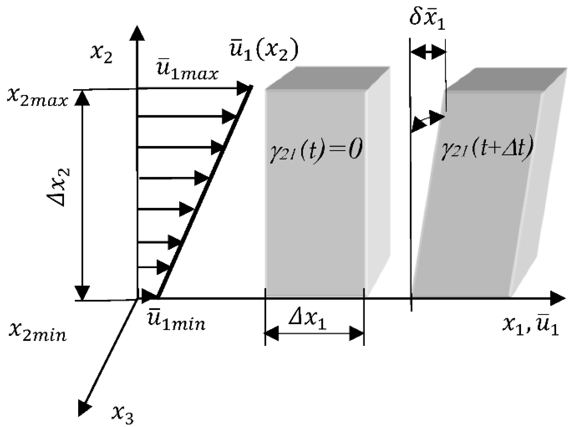
In 1687 in his Philosophiae Naturalis Principia, Isaak Newton [11] published the constitutive equation for steady two-dimensional laminar shear flows that is called Newton’s law of viscosity. To introduce it, we assume a flow with velocity in the —direction that is sheared in the perpendicular—direction and shows a (linear) velocity profile . Furthermore, the flow does not depend on the —direction ) (see Figure 1). Then, Newton’s law of viscosity states that the shear stress between fluid layers at coordinates and + is proportional to the spatial velocity derivative at location . For a given pressure p and absolute temperature T, the ratio of the shear stress to shear rate is a constant defining the dynamic viscosity of the fluid (see Equation (2) below). By substituting the relation for the generalized dynamic viscosity , where δ denotes the Dirac distribution, and the forcing field gradient into Equation (1), furthermore, applying the two simplifying conditions for shear flows: , and setting , the complex integral relation reduces to Newton’s single-term law of viscosity,

Figure 1.
Dynamic fluid deformation by the average velocity field of an element of an incompressible fluid participating in a laminar, transitional, or turbulent shear flow. Reprinted from Egolf and Hutter, 2019, Springer Edition Cham, Switzerland, reproduced with changes.
Note that in Equation (1) the Dirac distribution constricts the large-scale spatial dependence to a single point and makes the law local. Furthermore, for constant the relation is proportional to and, therefore, this law is also linear:
3.2. Some Results of the Kinetic Theory of Gases
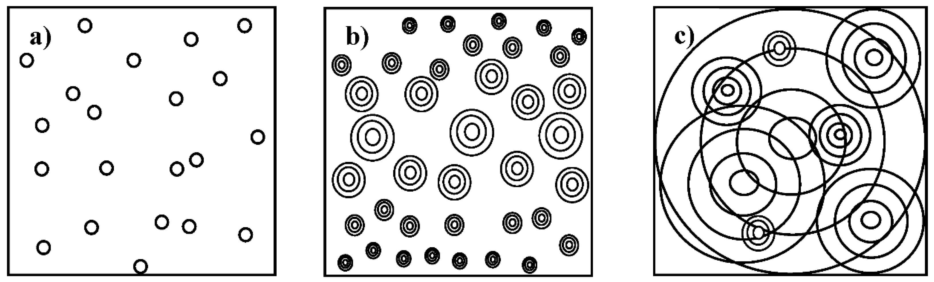
In a microscopic theory this important law can be derived by first physical principles of flying atoms or molecules, respectively obeying Brownian motion, that exchange momentum from the high-fluid-velocity regions to such of low velocity (see Figure 1). This theory is well established and is called the kinetic theory of gases. Because of space limits the derivation cannot be presented here (see, e.g., Reference [4]). However, one of its main results is the formula for the dynamic viscosity, being which contains the product of a characteristic length λ * (* following conventions in the physical literature, we leave away average and root mean square (rms) signs), being the mean distance between two collisions of molecules, also called mean free path length, and the characteristic (rms) flight velocity of the molecules *. The reason that the theory is valid in its linear form is that a single molecule’s diameter d is several orders of magnitude smaller than the mean free path length λ, that, on the other hand, is usually smaller than the size of the gas containing vessel L: d << λ << L (see Figure 2a).
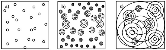
Figure 2.
(a) In the microscopic model of laminar flows in a channel molecules of a single diameter d are flying about with a mean free path length λ. In Boussinesq’s turbulence closure with a constant eddy viscosity the analogous mechanism occurs, there are moving eddies of only one size. (b) On the other hand, in Prandtl’s mixing-length model, where the eddy viscosity is dependent on the mean downstream velocity , the eddy diameter d also depends on the -coordinate (pointing in the vertical direction to the top) which leads to a stratification of eddies of different sizes (c) In a real turbulent flow (roughly sketched in this image) the situation is even more complex: momentum is transferred by a cascade of fractal eddies (for simplicity they are drawn circular with their mean discretized diameters ) and at each location eddies of many different sizes act simultaneously.
4. Constitutive Equations of Turbulent Flows
4.1. The Closure Problem
In fluid mechanics there are strong analogies between the constitutive equations of laminar and that of turbulent flows. However, there are also essential differences in these equations and their microscopic theories that must be explained in detail. We start with the momentum equation of fluid dynamics, also called Navier–Stokes Equation (NSE) [12]. After a proposal of Reynolds, the main three variables in this equation, namely the three velocity components, are split into two parts each: , where denotes an ensemble average (or in a quasi-steady flow the time average) and is its fluctuation quantity for which . Then, these two-fold velocities are substituted into the NSE and the average operator is applied to the entire equation. Formally, this produces the same equation as the NSE(), but now it depends on the averaged velocities, NSE() (why it is called Reynold’s Averaged Navier Stokes equation (RANS) [13]). As a result of this procedure, it also contains an additional term. Because of the quadratic products in the inertia terms of the NSE, with help of the mass conservation equation (continuity equation), the just described recipe produces nine additional second order correlations . These are regrouped to define a symmetric 3 × 3 tensor, being similar as the NSE’s dissipation tensor . Therefore, in analogy to the dissipation stress tensor, the additional turbulent stress tensor, also called Reynolds stress tensor, , is obtained. For this tensor, the general constitutive Equation (1) with an averaged driving term leads to the nonlocal and fractional derivative closure [14,15]
where, with the relation , the generalized turbulent kinematic viscosity , in turbulence research also called eddy viscosity (index m = momentum), was introduced. Note the formal equivalence of Equation (3) with the general definition of a fractional derivative, where the kernel or weighting function/distribution (in our case ) characterizes the type of the derivative; if it is, for example, a Riemann–Liouville function, the resulting fractional derivative is of Riemann–Liouville type, etc.
4.2. Kraichnan’s Direct Interaction Approximation (DIA)
It is highly satisfying that Kraichnan * (* Around 1950 Robert Kraichnan was one of the last assistants of Albert Einstein at Princeton University. He performed research on quantum field theories including the transfer of some of its ideas to the field of turbulence.) in his Direct Interaction Approximation (DIA)—by completely different means—also derived Equation (3) [16,17]. The output we got from the application of the Reynolds method is the new occurrence of six additional second order correlations for which no equations exist. Note that the three non-trivial symmetries, = , reduce the number of independent correlations from nine to six. There are two applied solutions to this problem. The first method is today most frequently applied in turbulence modeling: by manipulating the NSEs it is possible to introduce a whole cascade of higher order correlations and equations relating them up to the order infinity. Over the years a multitude of different methods for handling high order systems of equations have been developed. However, all these models are irrelevant to our purposes; we believe that they are not wrong, but possibly superfluous, why we here do not discuss them any further. The second method was introduced by early turbulence researchers: in their lowest order approach, the second order correlations are directly described by functions and/or operators of the first order mean values and . If these (or in Equation (3) all the generalized kinematic viscosities ) are known, they are substituted into the RANS equations and then the system of equations contains only mean first order variables or/and . By this the system of equations becomes closed and solvable. This is the reason why in turbulence research the equation is called a first order closure scheme. Now, it is recognized that the DQTM—which is a first order closure equation of turbulence and a zero-equation turbulence model * (* The name ‘zero-equation turbulence model’ stems from the absence of transport equations of the turbulent kinetic energy k, the dissipation rate ε or the vorticity ω, as they occur in high order turbulence models, for example, in the k-ε model or in the k-ω model.) (see Equation (5) below)—is analogous to constitutive equations in other areas of physics and, therefore, is the constitutive equation of turbulence. A small variation in the analogy is that the turbulent stress tensor is not dependent on the dynamic viscosity, determined by the molecules of the fluid; it depends on the analogous quantities which in turbulence are virtual particles called eddies. Therefore, this dynamic viscosity is called eddy viscosity, , and it is an apparent viscosity. The kernel in Kraichnan’s nonlocal stress tensor must be generalized by , where, as we will experience later, the dependence on the spatial variable with an apostrophe, , in this term, but not in the derivatives , may be removed. This replacement can be physically explained and motivated. In laminar flows the eddy viscosity is zero: = 0, . It is an increasing agitation (e.g., stirring or splashing) in the fluid that makes the eddy viscosity increase. So, the eddy viscosity is not a (constant) physical property, it is the result of the dynamics of the fluid. Therefore, it depends on the difference of the Reynolds numbers Re and : . With , where the characteristic length d and the fluid’s molecular viscosity are constant, in the difference of the Reynolds number only the velocity difference , in our case, is assumed to be a variable. In the eddy viscosity of a Reynolds stress the velocity must be Galilean invariant and, therefore, it only appears in velocity derivatives or differences, in which the constant critical velocity drops out. Therefore, the dependence holds. Finally, we hope that these arguments sufficiently convince also critical readers of the applicability of the above introduced replacement which was already applied in ancient times of turbulence research by numerous scientists, as, for example, Prandtl, Görtler, von Kàrmàn, Taylor, Wieghardt, etc. The dependence of the turbulent kinematic viscosity on the velocity makes the turbulent shear stress nonlinear (this is seen by a substitution of into Equation (3)), but not nonlocal. It is the integral representation of the Reynolds stresses in Equations (1) and (3) that is responsible for their nonlocal properties.
4.3. The Boussinesq Closure Approximation
Joseph Boussinesq was the first who modeled turbulent momentum transfer in analogy to molecular momentum transfer. This method led to a turbulent shear stress that we now derive by making use of our general approach (3). By applying an idea of Prandtl, is replaced by the eddy viscosity . Then this viscosity term, the averaged forcing field gradient and the same simplifying conditions as in the derivation of Newton’s viscosity law (see above), but now for the averaged velocities, are substituted into Equation (3) which, in analogy to Equation (2), yields:
With a constant eddy viscosity this is Boussinesq’s closure hypothesis. It is a linear and local “gradient” constitutive equation of turbulence which he published in 1877 [18]. The nonlinear version (4) also rests local and is still a main core part of present high order turbulence modeling work (see first method above). Therefore, one is not astonished that with this local approach so many problems in the past had occurred. To derive the correct constitutive equation of turbulence all conventional mathematical methods of physics * (* We exclude fractional calculus from the conventional methods of mathematical physics applied in the past. However, today in numerous fields of physics this calculus is becoming increasingly important and wider recognized. It slowly becomes exposed and evident that fractional calculus is also the right mathematical tool to describe Reynolds stresses of turbulent flows.) had failed which is one reason that Richard Feynman stated that turbulence is one of the most important remaining unsolved problems of classical physics [19], a judgment that is still true today!
4.4. Prandtl’s Mixing-Length Turbulence Model
The microscopic theory leading to closure (4) goes back to Ludwig Prandtl, who in 1925 published his mixing-length turbulence model [20]. As a result of the similarity of Equations (2) and (4), he applied the ideas of the kinetic theory of gases to derive a kinetic theory of turbulence. We do not present the development of the model by Prandtl, but will demonstrate an analogy of the two approaches in a very brief manner. Prandtl’s derivation led him to the following result for the eddy viscosity . Here l denotes the mixing length of the turbulent momentum transfer by the eddies. Rewritten this equation yields: . This is the analogous result to of the kinetic theory of gases (the constant 1/3 may be thought to be absorbed by l). The mixing length of the eddies l is analogous to the mean free path length of the molecules λ and as the molecules have their characteristic velocity also the eddies show such a velocity, . From the second last equation, we see that, if the eddy viscosity and the mixing length l are constant, has a single value and is also constant. In research of turbulence, it is a well-known fact that there is a strong monotonic power law dependence between the eddy diameter and the eddy velocity. Therefore, a single eddy velocity corresponds to a single eddy size. As a result, one has a strong analogy between this turbulence model and the kinetic theory of gases, presented in Figure 2a. In this figure, one may replace the molecules by small single-size eddies. In this simplest approach, a single class of eddies of equal size transfers all the turbulent momentum which is surely not a realistic image of real facts. In a slightly generalized turbulence model, the velocity depends on the spanwise coordinate of the flow. As a result of the strong monotonic relation the eddy size is now also —dependent. Figure 2b shows a picture of the eddies of this generalized turbulence model, where they are of multiple sizes and show a stratification. This is a good step toward a more successful turbulence model. However, studying drawings by Leonardo Da Vinci of turbulent flows [13] shows that he already had recognized that the situation in these flows is even more complex. As shown in Figure 2c, he had drawn pictures of interpenetrating eddies of multiple sizes, that act simultaneously at a given point. In the past the first author had taken this picture as a guideline to develop a ‘microscopic theory’ of turbulence leading to the DQTM (see [13,21,22]). The main idea was to realize a modeling of turbulent momentum transfer based on multi-size, self-similar and fractal eddies [23].
4.5. The Difference-Quotient Turbulence Model
To discover the constitutive equation of turbulence, one may make a hypothesis and then prove it by a microscopic theory. In the development of Newton’s law of viscosity, a Dirac distribution occurs which leads to the (most) local description. Thinking innovatively, we may now ask the question: “In the opposite case, which kernel leads to the least possible locality?” In Kraichnan’s nonlocal model is usually a decaying function of the distance between two points in space, . Fact is that the less the decrease is, the more nonlocal the problem will be. Therefore, a kernel, described by a Heaviside distribution , that in a fluid carrier domain is 1 (constant) and outside 0 (zero), shows the least decay and leads to the strongest nonlocal approach and this shall be further investigated. Now, we assume a generally large one-dimensional domain (see Figure 1). The position where the averaged velocity is at its minimum is , and where it is at its maximum it is , . With an eddy viscosity dependent on the down-slope diffusivity regime and a driving force dependent on the up-slope driving region , we postulate a generalized eddy viscosity to be: . Furthermore, we keep to the driving field and assume simplifying conditions similar as those in the derivation of Equation (4). Now, the integration interval can be reduced from the entire flow domain to , because in the interval the Heaviside integrand is zero. On the other hand, in the reduced region it is equal to unity. Therefore, in the restricted integral of Equation (3) the spatial integration directly acts on the derivative of the average velocity leading to . By this the integration simply produces the velocity difference of the mean velocities evaluated at the two bounds, , of the integral: . In the denominator with a similar integral (with the same Heaviside carrier domain, but without a velocity derivative), the normalization condition leads to: . Substituting these results into Equation (3), with analogies to the derivation of Equation (4), the constitutive equation of turbulence occurs
with σ being a constant. The modified turbulent kinematic viscosity, in analogy to the kinetic theory of gases, was set to be . Also in this expression, we can recognize the product of a typical length (scale) , that now can be a large-scale nonlocal quantity, because it varies between 0 and which may span the entire flow domain, and the averaged velocity difference which at takes its maximum, . Note that, just as gradients, space and velocity differences are Galilean invariant. It is remarkable that the nonlocal Difference-Quotient Turbulence Model [1,24]—which was discovered by completely different ideas—coincides with the constitutive equation of turbulence (5). This equation has a geometrical interpretation [13,25]. The Reynolds stress is proportional to the shear velocity: (see Figure 1). Therefore, with t and , it follows that
and by combining two of the above equations with Equation (5) directly follows. Note that instead of the limes the limes toward the value applies which is a quantity that tends toward its maximum to a large-scale spatial difference. Note that in the difference quotient the velocity may be nonlinear in . Nonlinearity of the Reynolds stress in appears only in the combination of the generalized eddy viscosity, , with the difference quotient.
4.6. A ‘Microscopic Theory’ of Turbulence
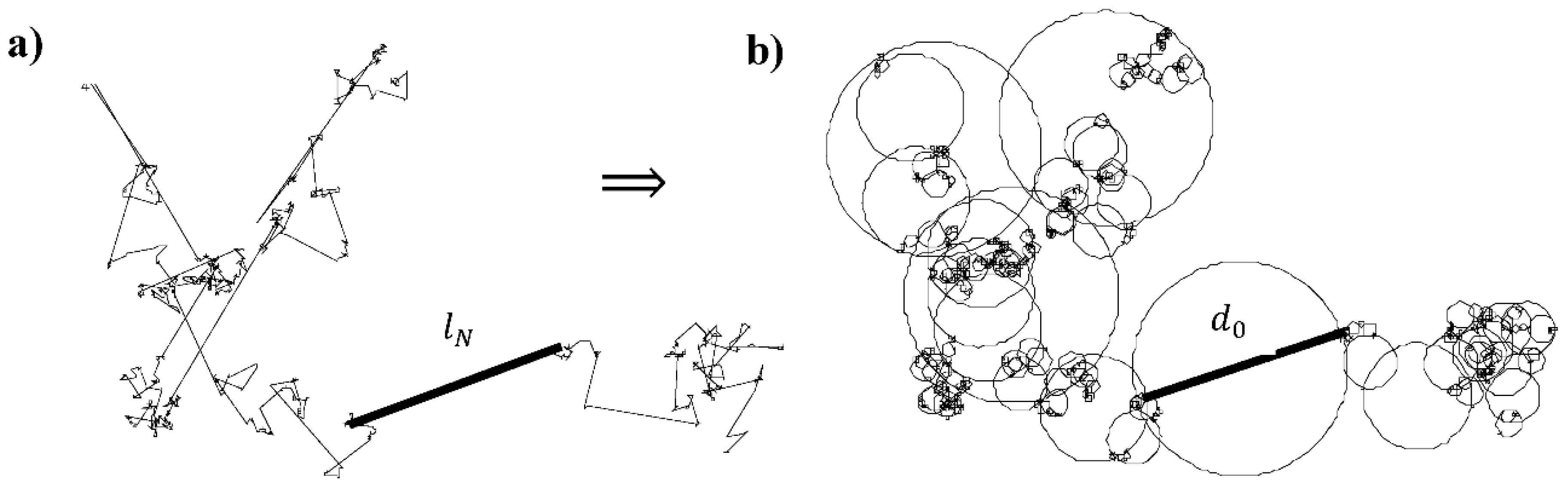
It is tempting to derive the constitutive law of turbulence (5) also by a ‘microscopic theory’. Because of space reasons, we can only sketch this theory by discussing the main ideas. A reader interested in the probabilistic/statistical details is guided to references [13,21]. In a turbulent flow, the higher its forcing and the lower the viscosity of the fluid are (high Reynolds number), the smaller will be the size of the smallest eddies. Kolmogorov’s dissipation length defines the low-wave-length cut-off value of the eddy probability distribution [26]. Eddies with diameters smaller than this length dissipate their turbulent kinetic energy immediately into heat. Therefore, the smallest eddies are not microscopic like atoms and molecules, but they still may be exceedingly small. On the other hand, the largest eddies may have a size comparable to the overall flow domain (see Figure 2c) which is macroscopic. Therefore, we classify this theory to be more a meso-macroscopic model *(* To keep the analogy also of the name to the molecular case, we denote this theory ‘microscopic theory,’ where the apostrophes shall remind us of the highly stressed use of this terminology.) than a microscopic one as, for example, the analogous kinetic theory of gases. To build this theory, at first for a quasi-steady turbulent flow the steady state of the spatial eddy distribution is required which we call the space occupation number of eddies. Other than for the molecules, for which we assume a birth rate zero (a certain number is already present and rests constant) and lifetimes which are infinite, in a turbulent flow field eddies are frequently born and die again. Advantageous is that in the field of mathematics and turbulence a theory of the birth rates of eddies, namely Lévy statistics [5], and a theory of their lifetimes, the fractal β-model [6], have been developed, so that they only must be combined. It is appropriate to identify the lifetimes of eddies with their turnover times. Now, we split up the eddies into discrete classes n with eddies of multiple sizes , where denotes the diameter of the largest and of the smallest eddies of a cascade. The combination of these two theories leads to the occupation number of eddies of class n, , and O is the total sum of all eddies. In this modeling the main relations are self-similar power laws which in their exponents also contain the Euclidean dimension D and the fractal or Hausdorff–Besicovitch dimension d, respectively. Then, the momentum transfer of eddy class n to the neighboring class n+1 is determined, leading to a result of impressive simplicity: [21]. The momentum transfer depends only on the quantity a which is the mean number of Lévy flights of length that occurs before a rarer flight of length is observed, the dimensionless flight length of the smallest flights, b > 1, the number of the class of Lévy flights (see Figure 3a), n, and the turbulent momentum transfer of the largest eddies, . To obtain the total momentum transfer at a certain space location this simple scaling relation adds up for a part of the as the development of model (5) [22] requires. The summations of the self-similar expressions lead to results that contain amplification factors times the momentum transfers only of the eddies being members of the largest classes which at maximum are . These amplification factors mathematically represent the action of all medium and smaller scale eddies (see Figure 3b) with the result that in the constitutive Equation (5) only two large scales are observable. However, this does not mean that only large eddies are transporting momentum; all eddies of smaller sizes are also actively and simultaneously at work by transferring momentum in the —direction. Studying this equation, we see that the largest eddies’ size depends on the coordinate which is very meaningful as, for example, the active eddies at a location above a wall, which is positioned at (by the no-slip boundary condition the mean velocity at the wall is zero: ), can only have the maximum size being identical to the distance from the wall.

Figure 3.
(a) The basic idea of a ‘microscopic theory’ of turbulence is the application of Lévy flights that here are shown in a two-dimensional image where two thousand flights were printed. (b) Each Lévy flight trajectory in Figure 3a defines the diameter of a corresponding eddy in Figure 3b. The thick line in Figure 3a shows a largest Lévy flight of class N: corresponding to the diameter of the largest eddy of class 0: (thick line in Figure 3b) with . The opposite indexing from small to large sizes in the Lévy statistics ( ) and in turbulence research ( ) is a result of the fact that the concepts were developed in different areas of physics. The eddy distribution shows typical self-similar clustering, leading to areas of a low eddy density and such of high density producing intermittent spottiness (see bright calm and dark whirling regions) as it occurs in turbulent flows. Note that this is a discretized eddy representation of a continuous eddy distribution in real space. Reprinted from Egolf, 2009, Int. J. Refr., reproduced with changes.
4.7. Analytical Solutions of Elementary Turbulent Flow Problems
4.7.1. Introduction
With the new constitutive equation of turbulence (5), the following elementary turbulent shear flows have analytically been solved (where each example listed is accompanied by the corresponding reference where the flow problem was solved): the turbulent flow in the wake behind a cylinder [24], the axisymmetric turbulent jet into a quiescent surrounding [24,27] and into a high-velocity constant co-flow [24], plane turbulent Couette flow [28] and plane turbulent Poiseuille flow [29] and finally the turbulent flow parallel to a wall [21]. To convince readers of the power of the new constitutive equation, in Section 4.7.2, Section 4.7.3, Section 4.7.4 and Section 4.8 we present three elementary flow problems with their essentials and solutions.
4.7.2. Turbulent Wake Flow
The turbulent wake flow behind a cylinder is in a certain sense special, because it is possible to derive its Reynolds shear stress by rigorous physical methods. To calculate the drag on a cylinder in a parallel flow in the —direction, the mass (continuity) and the momentum conservation equation (NSE) are applied in their integral forms. This leads to the following rigorous physical relation [24,30]
where is the density of the incompressible fluid, p is a pole distance upstream of the cylinder’s center and the constant upstream velocity of the parallel horizontal main flow in the —direction. It is highly satisfying that this result reveals the same large-scale difference in space, , and mean velocity difference, , which also appear in Equation (5); but more than this, if Equation (5) is applied to the wake flow problem and an order-of-magnitude approximation is taken into consideration, the DQTM rigorously produces this Reynolds shear stress [24]. To the authors best knowledge, until today the DQTM is the only turbulence model that produces this first-physical-principle Reynolds stress and this even with the right multiplicative constant! The lack of any gradient in this Reynolds shear stress and the occurrence of nonlocal large-scale spatial lengths and averaged velocities, as occurring in Equation (5), show that nonlocal and fractional calculus is the right choice to close turbulent flow problems with a corresponding constitutive equation of turbulence.
4.7.3. The Turbulent Axisymmetric Jet
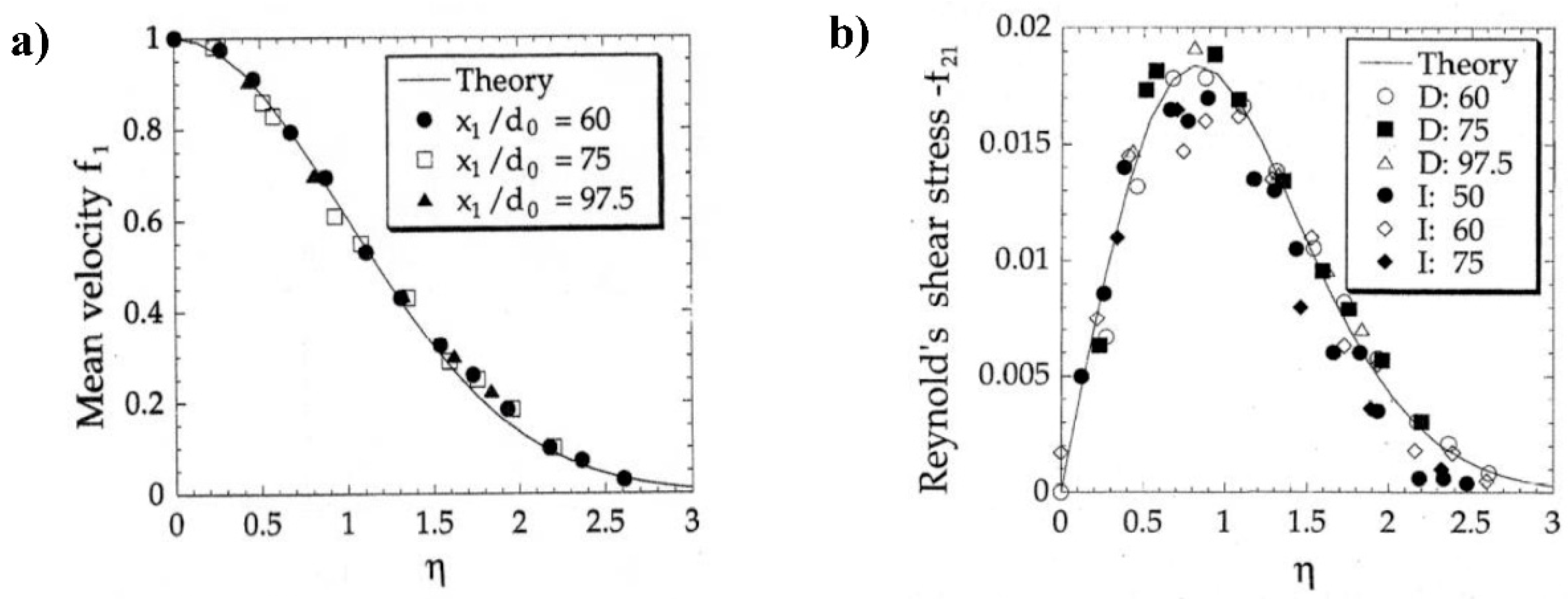
In this section, we study an axisymmetric turbulent jet flow into a quiescent surrounding, where the —direction is identical to the round jet’s axis (the detailed calculations are in Refs. [24,27]). The flow width of the jet from a virtual origin behind the nozzle linearly increases with . Now, the radial spatial coordinate is normalized by the expression . Furthermore, the average downstream velocity is made dimensionless by with its value on the jet axis, , where the mean velocity shows its maximum (see in Figure 4a the right half of the symmetric mean velocity profile with its maximum at η = 0). By combining the two partial differential equations (the continuity equation and the NSE) with the new closure of turbulence (5) which is a difference equation, substituting and the self-similar coordinate and function , the quasi-two-dimensional flow problem becomes one-dimensional which is essential to determine analytical solutions of this turbulent flow problem. By this procedure, the following highly nonlinear ordinary differential equation results:
where an apostrophe, , denotes the derivative d/dη. Its solution is the Gaussian function which is self-similar with respect to the dimensionless coordinate in the transverse direction and the mean downstream velocity and represented by the equation
(see Figure 4a). By a substitution of Equation (9) into differential Equation (8), a reader may prove this by her-/himself. Note the extraordinary complexity of the highly nonlinear differential Equation (8) and, on the other hand, the high simplicity of its solution (9).
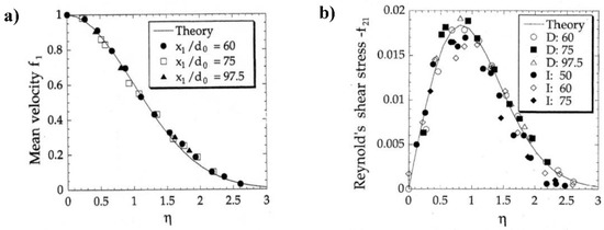
Figure 4.
(a) Theoretical solid line curve calculated with the DQTM and experimental data symbols from Reference [31] of the average axial (downstream) velocity in the radial direction for different downstream locations. The measured points lie close to the Gaussian function. (b) Reynolds shear stress with two types of experimental results D (Direct) and I (Indirect) (see main text). Just as in (a), also in this case the agreement between theory and experiments is excellent. Reprinted with permission from Egolf and Weiss (1998) © 2021, American Physical Society.
The dimensionless Reynolds shear stress is directly derivable from Equation (5) and is
which is shown as Figure 4b. In the figure inset “D” denotes direct experimentally measured values of and “I” are measurements of , shown in Figure 4a, which, by applying Equation (10), describing the Reynolds shear stress, were transformed to give indirectly (I) further values of . The mean velocity and the Reynolds shear stress show an excellent agreement between the theoretical data [24] and the experimental observations by Wygnanski and Fiedler [31] (see Figure 4a,b). Also, excellent quality is obtained for the three normal Reynolds stresses, the turbulent kinetic energy, the production and dissipation of turbulent kinetic energy and the turbulent convection (see References [12,13,27]).
4.7.4. Plane Turbulent Couette Flow
This type of flow is created by shearing two parallel plane plates of distance 2a with a fluid in between by keeping the lower plate at rest and moving the higher positioned one with velocity U > 0 in the positive —direction. In the laminar case this is the prototype flow to demonstrate Newton’s law of viscosity. It is well-known that the continuity and a reduced and linearized Navier–Stokes equation, supplemented by the constitutive equation of Newton (Newton’s law of viscosity), lead to a linear differential equation and a linear velocity profile between the two different velocities of the plates (see Table 1). Note that (because of the no-slip boundary condition) the plate velocities are identical to the fluid velocities at the boundaries of these plates, where the dimensionless mean velocity fulfils the boundary conditions given as Equation (11). In these equations , where a is the half distance between the two plates. If instead of Newton’s law of viscosity the DQTM is implemented—in this more general case—into the nonlinear, self-similar NSE, one obtains the following quadratic differential equation with the two boundary conditions (these and further following results and their calculations are found in [28])

Table 1.
Analogies between laminar and turbulent flow constitutive equations and their solutions for plane laminar and turbulent shear Couette flows.
The solutions of the time-averaged turbulent velocity profiles are S-shaped curves (an example is shown in Figure 5a by the full line). With the dimensionless averaged downstream velocity and the relation , it is described by the following equation:
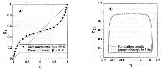
Figure 5.
(a) Comparison of the theoretical mean velocity profile (see Equation (12) with β = 3.8 and α from Equation (13) or Figure 6, respectively) with experimental data from Reference [32]. The mean velocity profile is nonlinear and S-shaped (here in a mirrored picture). In the infinite Reynolds number limit the distribution is a constant , fulfilling the boundary conditions (11) by the occurrence of two discontinuities at the boundaries. (b) In the second figure a comparison of the theoretical Reynolds stress (see Equation (14) below with β = 3.96 and α from Equation (13) or Figure 6, respectively) with numerical simulation results from [33] is presented. In the infinite Reynolds number limit the distribution is a constant , fulfilling the boundary conditions by the occurrence of two discontinuities at . Reprinted with permission from Egolf and Weiss (1995a) © 2021, American Physical Society.
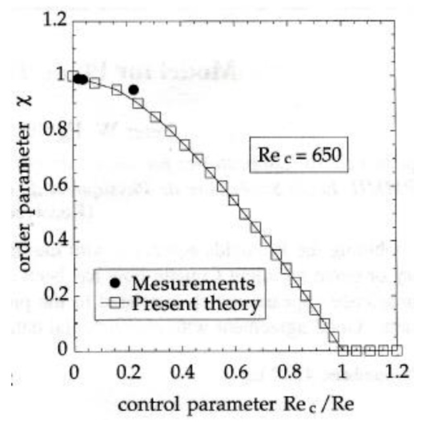
In the mathematical process of determining solution (12), the relation between α and β is revealed. The parameter α is the stress parameter (control parameter) of the flow system, which is tightly related to the Reynolds number, and the second parameter β, respectively χ (normalized β), is the systems order parameter (see Figure 6). This mathematically derived order parameter relation is

Figure 6.
Order parameter χ, determined by Equation (13) and compared with experimental results from Reference [32]. There is a lack of good experimental results at excitations just slightly above the criticality. This is explained by the inverse relation between α and Re and the difficulty for experimentalists to perform good experimental set-ups and experiments to measure the turbulent fields at values just slightly above the critical Reynolds number (for more details see in Reference [28]). Reprinted with permission by Egolf and Weiss (1995a) © 2021, American Physical Society.
By decreasing the Reynolds number, Re, from high values down toward the critical Reynolds number, ReC, these mean velocity profiles loose curvature and converge to the linear laminar profile (see Figure 5a, the linear function is represented by a dashed line). One may easily show that for the Reynolds shear stress the DQTM directly leads to the formula . By a substitution of the right-hand side of Equation (12) into this equation, it follows that
which is shown together with numerical data from Reference [33] as Figure 5b.
4.8. Turbulence: A Critical Phenomenon
In turbulent flow fields universality of rare fluctuations were experimentally observed and a lack of theory of critical phenomena of turbulence [34,35] was occasionally complained (see e.g., Refs. [36,37]). Analytical solutions, derived by an application of the DQTM, in a natural manner reveal theories of critical phenomena with criticalities and in which the two phases of the fluid are the low-entropy vorticity-rich regions and the high-entropy laminar streaks. Transition from laminar to transitional and turbulent flows at critical Reynolds numbers are known since the time of Osborne Reynolds (1842–1912). Theoretical vortisation curves * (* The name vortisation was proposed by the authors [25] from the word vorticity, in analogy to the name magnetisation which both are order parameters as function of related stress parameters of the respective physical systems.), in analogy to magnetisation curves in magnetism, have been determined for numerous turbulent flow types. Figure 6 presents the vortisation curve of plane turbulent Couette flow.
In References [13,38], in analogy to the mean field theory of magnetic materials, a mean field theory of turbulence was developed. The results are meaningful and accurate. This is explained by the fact that a quasi-steady turbulent flow, with a constant turbulent kinetic energy flow into and out of the system’s Kolmogorov energy cascade, leads to behavior that is very similar to that of physical systems in thermodynamic equilibrium. In analogy, a Curie law of turbulence and a Curie–Weiss law of turbulence were discovered. From the Curie law of turbulence, in analogy to the Curie law of magnetism, the turbulence intensity has been determined to be the response function of turbulence, as, for example, compressibility is of a gas and susceptibility of a para-ferromagnetic phase-change material. Note that results of fluid dynamic considerations—involving the Difference-Quotient Turbulence Model (DQTM)—leading to critical phenomenon, are of higher physical relevance than results extracted only from an ad hoc model like the mean field theory of turbulence.
4.9. The Analogy between Laminar and Turbulent Flows
First order turbulence modeling has the great advantage that it follows the widely accepted method of introducing a generally valid constitutive equation to solve physical problems, as it is convention in other areas of physics. This is also the method of treating laminar flows, namely by applying Newton’s law of viscosity. In turbulence, we propose the introduction of a new nonlinear, nonlocal and fractional constitutive equation, which was discovered in April 1985 and is called the Difference-Quotient Turbulence Model (DQTM). Some results stemming from the application of this model to the elementary plane turbulent Couette flows are presented in Section 4.7.4. They show strong analogies to the laminar case which in this section both are outlined and compared in Table 1.
As may be seen in Figure 6, at criticality , the order parameter is χ = 0. If these values are introduced into the differential equation describing turbulent plane Couette flows (see in Table 1, third line, sixth row), it follows that . This is the differential equation for laminar plane Couette flows (third line, fifth row) and leads to the correct linear velocity profile (fifth line, fifth row), fulfilling the boundary conditions (11) (see also in Table 1, fourth line, fifth and sixth row).
5. Conclusions
This article promotes nonlocal and fractional calculus to model Reynolds shear stresses with a first order turbulence closure scheme and makes a new proposal for a constitutive equation of turbulence. This equation, in the limit of the Reynolds number converging to its criticality from above, conserves the full information of Newton’s law of viscosity of laminar flows. It also extends Boussinesq’s and Prandtl’s models of turbulent momentum transfer by a generalization from eddies of a single size to such of a cascade with numerous classes of fractal eddies of multiple sizes. Six applications of the Difference-Quotient Turbulence Model, DQTM (constitutive equation of turbulence) to elementary turbulent flow problems lead to analytical results which, compared with experimental and (direct) numerical simulation results, are of convincing precision. All the derived non-empirical analytical solutions are of high simplicity and accuracy.
Author Contributions
Conceptualization, P.W.E.; validation, P.W.E. and K.H.; formal analysis, P.W.E. and K.H.; investigation, P.W.E. and K.H.; writing—original draft preparation, P.W.E.; writing—review and editing, P.W.E. and K.H. All authors have read and agreed to the published version of the manuscript.
Funding
This research received no external funding.
Acknowledgments
We are grateful to Thomas F. Stocker (climatologist, University of Berne, Switzerland) for arranging and motivating our collaboration. Furthermore, we thank an anonymous reviewer for his helpful remarks.
Conflicts of Interest
The authors declare no conflict of interest.
References
- Egolf, P.W. A new model on turbulent shear flows. Helv. Phys. Acta 1991, 64, 944–945. [Google Scholar]
- Schlichting, H. Boundary-Layer Theory; McGraw-Hill Inc.: New York, NY, USA, 1979. [Google Scholar]
- Oldham, K.B.; Spanier, J. The Fractional Calculus; Academic Press: New York, NY, USA, 1974. [Google Scholar]
- Reif, F. Physikalische Statistik und Physik der Wärme; Walter de Gruyter: Berlin, Germany, 1975. (In German) [Google Scholar]
- Lévy, P. Calcules des Probabilités; Gauthier Villars: Paris, France, 1925. (In French) [Google Scholar]
- Frisch, U. Turbulence—The Legacy of A.N. Kolmogorov; Cambridge University Press: Cambridge, UK, 1995. [Google Scholar]
- Barenblatt, G.I. Scaling, Self-Similarity, and Intermediate Asymptotics; Cambridge University Press: Cambridge, UK, 2005. [Google Scholar]
- Pomeau, Y.; Manneville, P. Intermittent transition to turbulence in dissipative dynamical systems. Commun. Math. Phys. 1980, 74, 189–197. [Google Scholar] [CrossRef]
- Metzler, R.; Klafter, J. The random walk’s guide to anomalous diffusion: A fractional dynamics approach. Phys. Rep. 2000, 339, 1–77. [Google Scholar] [CrossRef]
- Foias, C.; Manley, O.; Rosa, R.; Temam, R. Navier-Stokes Equations and Turbulence; Cambridge University Press: Cambridge, UK, 2001. [Google Scholar]
- Newton, I. Philosophiae Naturalis Principia Mathematica; Jussu Societatis Regiae ac Typis Josephi Streater: London, UK, 1687. (In Latin) [Google Scholar]
- Hutter, K.; Wang, Y. Vol 2, Advanced Fluid Dynamics and Thermodynamic Fundamentals. In Fluid and Thermodynamics in Geophysical Context; Springer: Berlin, Germany, 2016. [Google Scholar]
- Egolf, P.W.; Hutter, K. Nonlinear, Nonlocal and Fractional Turbulence; Springer International Publishing: Cham, Switzerland, 2019. [Google Scholar]
- Hamba, F. Nonlocal analysis of the Reynolds stress in turbulent flows. Phys. Fluids 2005, 17, 115102-1–115102-9. [Google Scholar] [CrossRef] [Green Version]
- Egolf, P.W.; Hutter, K. Fractional Turbulence Models. In Progress in Turbulence VII; Springer: Cham, Switzerland, 2017; Volume 196, pp. 123–131. [Google Scholar]
- Romanof, N. Non-local models in turbulent diffusion. Z. Meterol. 1989, 39, 89–93. [Google Scholar]
- Kraichnan, R.H. Direct-interaction approximation for shear and thermally driven turbulence. Phys. Fluids 1964, 7, 1048–1062. [Google Scholar] [CrossRef]
- Boussinesq, J. Mémoires présentés par divers savants à l’Académie des Sciences. In Essai sur la Théorie des Eaux Courantes; Imprimerie Nationale: Paris, France, 1877; Volume 23, pp. 1–680. (In French) [Google Scholar]
- Vergano, D. Turbulence theory gets a bit choppy. USA Today, 10 September 2006. [Google Scholar]
- Prandtl, L. Bericht über Untersuchungen zur ausgebildeten Turbulenz. ZAMM J. Appl. Math. Mech. 1925, 5, 136–139. [Google Scholar] [CrossRef]
- Egolf, P.W. Lévy statistics and beta model: A new solution of “wall” turbulence with a critical phenomenon. Int. J. Refr. 2009, 32, 1815–1836. [Google Scholar] [CrossRef]
- Samba, F.K.C.; Egolf, P.W.; Hutter, K. Nonlocal Turbulence Modeling Close to Criticality Involving Kolmogorov’s Dissipation Microscales; Springer: Cham, Switzerland, 2017; Volume 226, pp. 163–170. [Google Scholar]
- Mandelbrot, B. The Fractal Geometry of Nature; W.H. Freeman and Company: New York, NY, USA, 1982. [Google Scholar]
- Egolf, P.W. Difference-quotient turbulence model: A generalization of Prandtl’s mixing-length theory. Phys. Rev. E 1994, 49, 1260–1268. [Google Scholar] [CrossRef] [Green Version]
- Egolf, P.W.; Hutter, K. Turbulent Shear Flow Described by the Algebraic Difference-Quotient Turbulence Model; Springer: Heidelberg, Germany, 2016; Volume 165, pp. 105–109. [Google Scholar]
- Hunt, J.C.R.; Phillips, O.M.; Williams, D. Turbulence and Stochastic Processes: Kolmogorov’s Ideas 50 Years On; The Royal Society: London, UK, 1991. [Google Scholar]
- Egolf, P.W. Difference-quotient turbulence model: The axi-symmetric isothermal jet. Phys. Rev. E 1998, 58, 459–470. [Google Scholar] [CrossRef] [Green Version]
- Egolf, P.W.; Weiss, D.A. A model of turbulent plane Couette flow. Phys. Rev. Lett. 1995, 75, 2956–2959. [Google Scholar] [CrossRef] [PubMed] [Green Version]
- Egolf, P.W.; Weiss, D.A. Difference-quotient turbulence model: Analytical solutions for the core region of plane Poiseuille flow. Phys. Rev. E 2000, 62, 553–563. [Google Scholar] [CrossRef] [PubMed] [Green Version]
- Hinze, J.O. Turbulence; McGraw-Hill Book Company: New York, NY, USA, 1975. [Google Scholar]
- Wygnanski, I.; Fiedler, H.J. Some measurements in the self-preserving jet. J. Fluid Mech. 1969, 38, 577–612. [Google Scholar] [CrossRef] [Green Version]
- Reichardt, H. Gesetzmässigkeiten der Geradlinigen Turbulenten Couette-Strömung; Mitteilungen aus dem Max-Planck-Institut für Strömungsforschung und der Aerodynamischen Versuchsanstalt (Selbstverlag): Göttingen, Germany, 1959. (In German) [Google Scholar]
- Lee, M.J.; Kim, J. The structure of turbulence in a simulated plane Couette flow. In Proceedings of the Eighth Symposium on Turbulent Shear Flows, Munich, Germany, 9–11 September 1991; Volume 1. [Google Scholar]
- Goldenfeld, N. Lectures on Phase Transitions and the Renormalization Group; Addison-Wesley Publishing Company: Boston, MA, USA, 1992. [Google Scholar]
- Ma, S.-K. Modern Theory of Critical Phenomena; The Benjamin/Cummings Publishing Company, Inc.: Reading, MA, USA, 1982. [Google Scholar]
- Bramwell, S.T.; Holdsworth, P.C.W.; Pinton, J.-F. Universality of rare fluctuations in turbulence and critical Phenomena. Nature 1998, 396, 552–554. [Google Scholar] [CrossRef]
- Castaign, B.J. Conséquences d’un principe d’extremum en turbulence. J. Phys. France 1989, 50, 147–156. (In French) [Google Scholar]
- Egolf, P.W.; Hutter, K. The mean field theory of magnetism and turbulence. J. Entropy 2017, 19, 589. [Google Scholar] [CrossRef] [Green Version]

Publisher’s Note: MDPI stays neutral with regard to jurisdictional claims in published maps and institutional affiliations. |
© 2021 by the authors. Licensee MDPI, Basel, Switzerland. This article is an open access article distributed under the terms and conditions of the Creative Commons Attribution (CC BY) license (https://creativecommons.org/licenses/by/4.0/).