Article

Computational Analysis of Lung and Isolated Airway Bifurcations under Mechanical Ventilation and Normal Breathing

1
Department of Radiation Oncology, University of Arizona, Tuscon, AZ 85724, USA
2
College of Engineering, University of Georgia, Athens, GA 30602, USA
*
Author to whom correspondence should be addressed.
Fluids 2021, 6(11), 388; https://doi.org/10.3390/fluids6110388
Submission received: 30 August 2021 / Revised: 14 October 2021 / Accepted: 20 October 2021 / Published: 29 October 2021
(This article belongs to the Special Issue Computational Biofluiddynamics: Advances and Applications)

Abstract

:
Mechanical ventilation is required for many patients who cannot breathe normally as a result of lung disease and other factors that result in reduced lung function. In this study, we investigated the effects of mechanical ventilation and normal breathing on whole lung geometry as well as isolated bifurcations through computational fluid dynamic (CFD) simulations. Results of flow characteristics (airflow velocity, wall pressure, and wall shear stress) obtained from the CFD simulations are presented. Similar flow patterns and pressure drops were obtained between the whole lung geometry and isolated bifurcations under both normal breathing and mechanical ventilation, respectively. Results obtained from simulations suggest that analyzing specific local bifurcations may be a more feasible alternative as it may reduce the computational time and numerical errors resulting from computations as compared to simulating a complex whole lung geometry. The approach presented in this study also demonstrated that analyses of isolated bifurcations gave similar flow characteristics to that of whole lung geometry. Therefore, this approach may be useful for quickly obtaining results that will assist in making clinical predictions and other applications.

1. Introduction

Mechanical ventilation is frequently administrated to help support breathing in patients with lung disease. For example, mechanical ventilation is used to assist breathing in some patients with potentially harmful lung diseases such as asthma and emphysema. Therefore, accurate knowledge of airflow characteristics under mechanical ventilation is critically important. The ability to efficiently model or simulate the airflow in the whole human lung offers a valuable alternative to costly and potentially harmful in vivo experimental methods. Evaluating airflow in the whole human lung airway, however, is complicated by several factors, including the limitations of existing imaging technologies, patient specific variations in lung morphology, and changes in airway geometry during the breathing cycle, not to mention the extreme size and multi-scale nature of the airway geometry [1]. The airway tree in the upper lung model is made up of successive bifurcating segments, comprised of approximately nine total generations, including approximately six in the bronchial region. The resulting geometry contains flow segments with diameters ranging from approximately 2 cm (trachea) to 0.13 cm. Previous computational fluid dynamics (CFD) studies of the human lung airway have focused on small subsections, for example, single [2,3] or triple [4,5,6] bifurcations. A few notable exceptions have addressed the large, multi-scale geometry of the entire tracheobronchial tree. These include both the whole and sequential simulations and the resolved multi-generation models.
There are a few other early studies of airflow in the lung airways, including the experimental test for the steady case [7,8,9], where a few velocity profiles and flow patterns were presented for a double-bifurcation model. In other experimental studies, the central airway up to the third generation of the bifurcation was used [10,11], but the respiratory flow was treated as a transient condition for both mechanical ventilation and normal breathing. Two important parameters that influence the fluid dynamics in an airway include the local geometry of the tracheobronchial (TB) tree and the inhalation and exhalation patterns. Most experimental and numerical studies on flow in the human airways have been based on simplified, idealized airway models, extracted from early morphological studies by Chang [12] and Horsfield et al. [13]. Van Ertbruggen et al. [14] used irregular dichotomy models based on morphometric data of Horsfield et al. [13], comparing their numerical results with experimental data [15], in terms of regional deposition efficiency. More recently, studies have explored flow and/or aerosol transport numerically in realistic airway models based on computerized tomography (CT) scanner imaging [16,17].
The objective of this study is to evaluate the airflow characteristics on whole lung geometry as well as isolated bifurcations through computational fluid dynamic (CFD) simulations under mechanical ventilation and normal breathing. Specifically, the goal is to evaluate the flow characteristics (velocity profile, pressure (resistance of breathing) drop, shear stress, and turbulent intensity (using vortex intensity)), and compare the results between the whole lung geometry and isolated bifurcations under both mechanical ventilation and normal breathing. The whole lung geometry model used by Xi et al. [16] was adapted and from which local/isolated bifurcations were built for CFD analysis. Realistic transient flow rates that are time-dependent were assumed. Positive constant velocity was assumed during inhalation and negative exponential velocity was assumed for mechanical ventilation, while positive sinusoidal velocity profile during inhalation and negative sinusoidal velocity profile during exhalation were assumed for normal breathing (see Figure 1a). The results of flow characteristics obtained from the CFD simulations are presented and discussed.

2. Methods

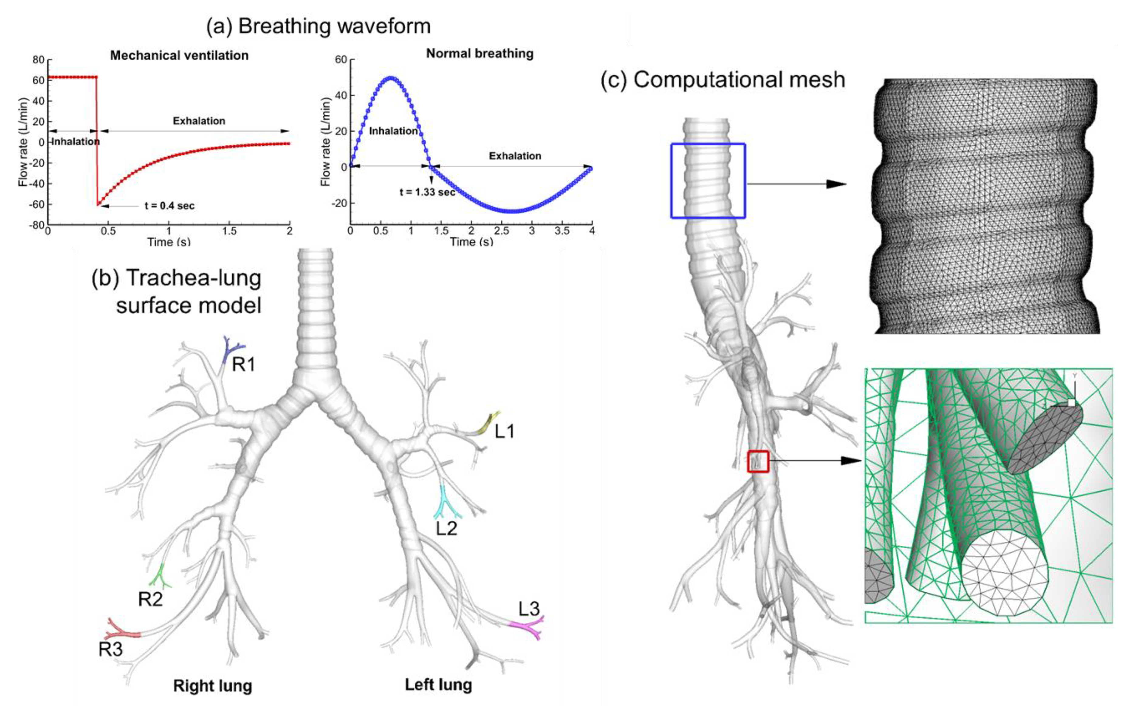
2.1. Construction of Tracheobronchial (TB) Model

An approximate TB whole lung model was digitally generated from MRI-CT data and used for the CFD analysis. The multi-slice CT images were imported into MIMICS (Materialise, Ann Arbor, MI) to convert the raw image data into a set of cross-sectional contours that define the 3-D solid structure. Based on these contours, surface geometry was constructed in Gambit 2.3 (ANSYS) (Figure 1b). The geometry considered in this study consists of the respiratory TB airways extending from the trachea to G9 bronchioles for the left and right side of the lung as shown in Figure 1b. The three major features of this physiologically realistic TB model are the right-left asymmetry, the cartilage rings, and non-planar aspect of bifurcating branches [18,19]. There are two lobes (upper and lower) in the left lung and three lobes (upper, middle, and lower) in the right lung. Similarly, ventilation to the right and left lungs is also asymmetric. In the resulting airway model, the trachea had an average diameter of 19 mm and a length of 90 mm. The diameters of the right and left main bronchi were 14.3 and 14.1 mm, and the lengths of the two bronchi were 23 and 57.5 mm, respectively. C-shaped cartilage rings were connected from TB model through the trachea to the bifurcation G4, which prevent these airways from collapsing during absence of air [20]. Surface properties of the bifurcations, such as the carina ridge, were taken from the measurements of Horsfield et al. [13] and Hammersley and Olson [21]. Several isolated bronchioles from the whole lung geometry were generated using the ANSYS Workbench (Figure 2b) and these were used for the analysis. All waveforms were scaled using cross-sectional areas and the generation number in the local bifurcation simulations.

2.2. Continuous and Discrete Phase Transport Equations

CFD studies of airflows inside an adult whole lung model were conducted using FLUENT software. The computational model for the upper lung had 9 generations with 115 outlets. It retained the cartridges on all bronchioles, and consisted of 3.5 million unstructured tetrahedral cells. A low Reynolds number (LRN) k-w turbulence model was employed to resolve the turbulence regimes. The Reynolds number of a flowing fluid is calculated by multiplying the fluid velocity by the internal airway diameter and then dividing the result by the kinematic viscosity. The mean Reynolds number varied from approximately 800 to 7987 during the transient cycle. The maximum Reynolds number based on peak inhalation or exhalation at the minimum cross section of the bronchioles was approximately 7987. A higher Reynolds number was observed in small bifurcations where high vortex occurs. Therefore, laminar, transitional, and fully turbulent conditions are expected in the TB airway model during the transient cycle. Hence, to resolve multiple flow regimes considered in this study, the low Reynolds number (LRN) k-w turbulence model where k is kinematic energy, and w is dissipation rate provided by Wilcox [22] and previously reported by Longest and Xi [23] was employed in the simulation. The LRN k-w model was selected based on its ability to accurately predict pressure drop, velocity profiles and shear stress for transitional and turbulent flows [24,25]. This model has also been demonstrated to accurately predict aerosol deposition profiles for transitional and turbulent flows in models of the TB airway [26,27] with multiple bifurcations [28,29]. Moreover, the LRN k-w model has been shown to provide an accurate solution for laminar flow as the turbulent viscosity approaches zero [25]. For the laminar and turbulent flow, the LRN k-w equations governing the conservation of mass and momentum given by Wilcox [22] were used:
u i x i = 0
u i t + u j u i x j = 1 ρ u i x i + x j v + v T u i x j + u j x i
where u i is the time-average fluid velocity in three coordinate directions (i.e., i = 1, 2, and 3), p is the time-averaged pressure, ρis the fluid density, and υ is the kinematic viscosity. The turbulent viscosity is defined as v T = α * k / w . For the LRN k-w approximation, which models turbulence through the viscous sublayer, the α * parameter in the above expression for turbulent viscosity is evaluated as noted in Wilcox [22]:
α * = 0.024 + k / 6 v w 1.0 + k / 6 v w

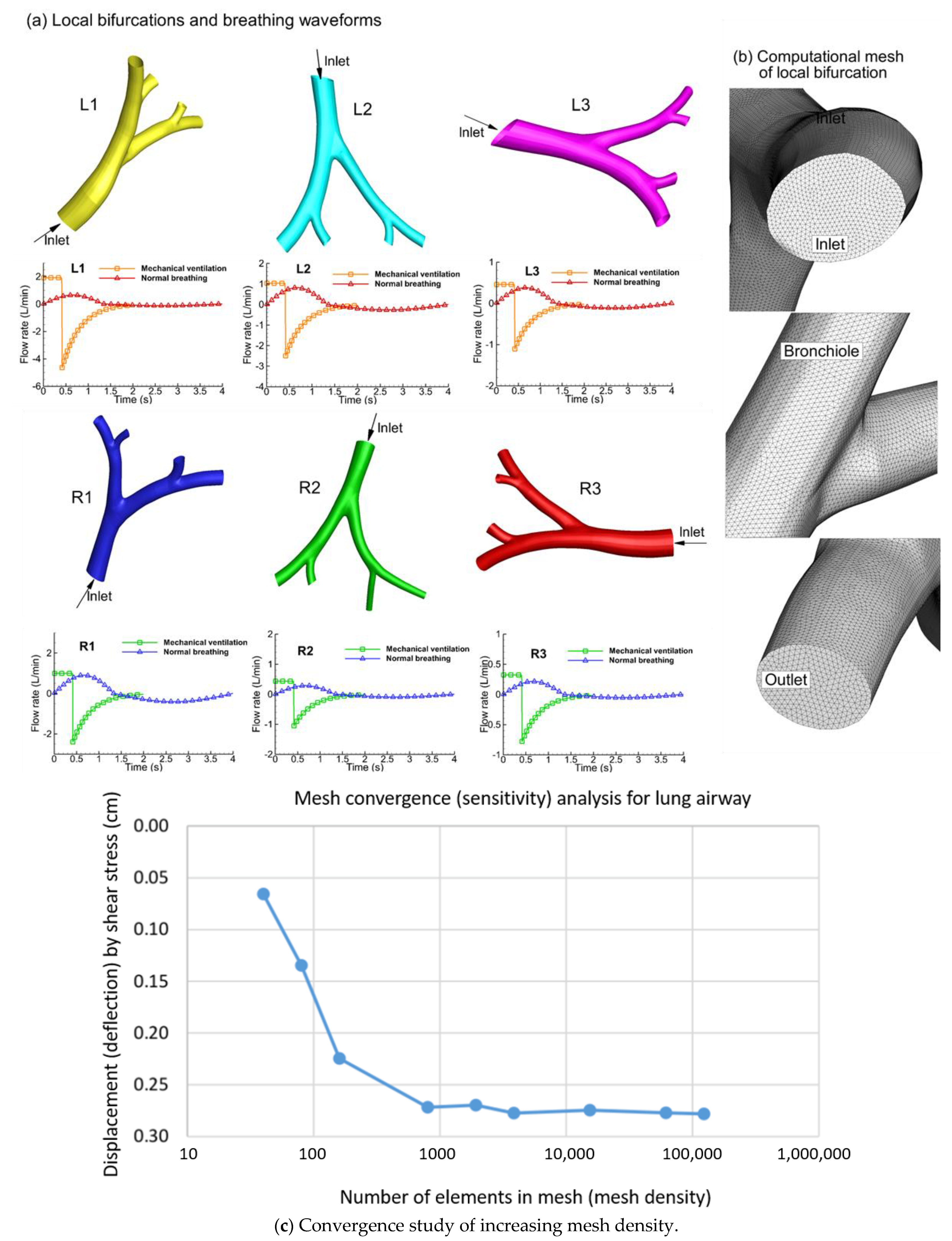
2.3. Flow Rates and Boundary Conditions

The CFD problem is defined under the limits of initial and boundary conditions. Boundary conditions are implemented by adding an extra node across the physical boundary. The nodes just outside the inlet of the system are used to assign the inlet conditions and the physical boundaries coincide with the scalar control volume boundaries. This makes it possible to introduce the boundary conditions and achieve discrete equations for nodes near the boundaries with small modifications. The experimental model of Cohen et al. [30] was implemented, and a transient sinusoidal waveform was obtained over multiple breath cycles. For the computational simulations in the previous study, both steady and transient (tidal) ventilation conditions were employed, and the transient breathing conditions were approximated as sinusoidal functions with the format [23],
Q t = Q i n 1 cos 2 w t
u t = u m e a n 1 cos 2 w t
where w is the breathing frequency in radians/s, Qin is inhaled flow rate and umean is mean velocity. Cohen et al. [30] reported measurements of flow characteristics at a mean cyclic flow rate of 34 L/min Q i n = 567   cm 3 / s and a breathing frequency of 20 breaths per minute w = 2.1   radians / s . A factor of transient condition in the previous study was included in the time varying portion of Equations (1) and (2) to match the experimental inlet conditions. This factor results in a respiratory cycle for each of the 20 breath periods per minute. As a result, the in vitro and numerical inhalation time is equal to the inhalation portion of a complete breathing cycle in vivo. To numerically approximate this transient inlet condition, a single cycle of flow initialization was subsequently followed.
Transient (tidal) conditions and waveforms for the whole lung model (see Figure 1a) under normal breathing and mechanical ventilation were considered for computational simulations. Under mechanical ventilation, there was a positive constant velocity during inhalation (0–0.4 s) and negative exponential velocity pattern during exhalation (0.4–2 s). The constant rate is determined such that, during inhalation, the lung takes in a total of 420 mL of air. In the normal breathing model, positive sinusoidal velocity profile was obtained during inhalation (0–1.33 s) and a negative sinusoidal velocity profile pattern was obtained during exhalation (1.33–4 s). This waveform gives rise to an overall intake of 700 mL in the lungs during inhalation. These breathing waveforms were calculated using a transient user-defined function with mechanical ventilation and normal breathing parameters summarized in Table 1. The calculated velocity profiles of a transient breathing waveform using the parameters from Table 1 are
u t = Q / F A 2 n 1
u t = Q exp ( t / 0.4 ) / F A 2 n 1
u t = 826.73 10 6 sin ( 2.3621 t ) / F A 2 n 1
u t = 411.82 10 6 sin ( 1.1766 t ) / F A 2 n 1
where Q is flow rate (tidal volume/inhalation time), t is flow time of either inhalation and exhalation, F(A) is total face area that is calculated by accumulating the magnitude of each face’s area units defined in Fluent, and n is generation number. Equation (6) is used for inhalation during mechanical ventilation, and Equation (7) is used for exhalation (0.4 < t ≤ 2) during mechanical ventilation. Equation (8) is used for inhalation (0 < t ≤ 1.33) under normal breathing, and the last equation is used for exhalation (1.33 < t ≤ 4) during normal breathing. In a similar manner, the waveforms of isolated bifurcations were represented by UDF with tidal volume conditions (see Figure 2a). This profile of inhalation under mechanical ventilation occurred under a constant velocity, and all profiles provided a smooth transition to the no-slip wall condition. The model outlets were extended 115 hydraulic diameters downstream such that the velocity was normal to the outlet planes (i.e., nearly developed flow profiles with no significant radial velocity component). The selected points of time steps for comparing mechanical ventilation and normal breathing were determined based on similar matching between time steps (for example, t = 0.3 s is the three fourths for flow time (0 s–0.4 s) for inhalation under mechanical ventilation, and it matches the three fourths on the t = 1.0 s for flow time (0 s–1.33 s) for inhalation under normal breathing). However, the flow rate for exhalation under mechanical ventilation at t = 1.2 s is approximately 18 L/min, which is the typical quiet breathing rate for an adult, and it matches at t = 3.5 s (see Figure 1a breathing waveform) for exhalation under normal breathing.

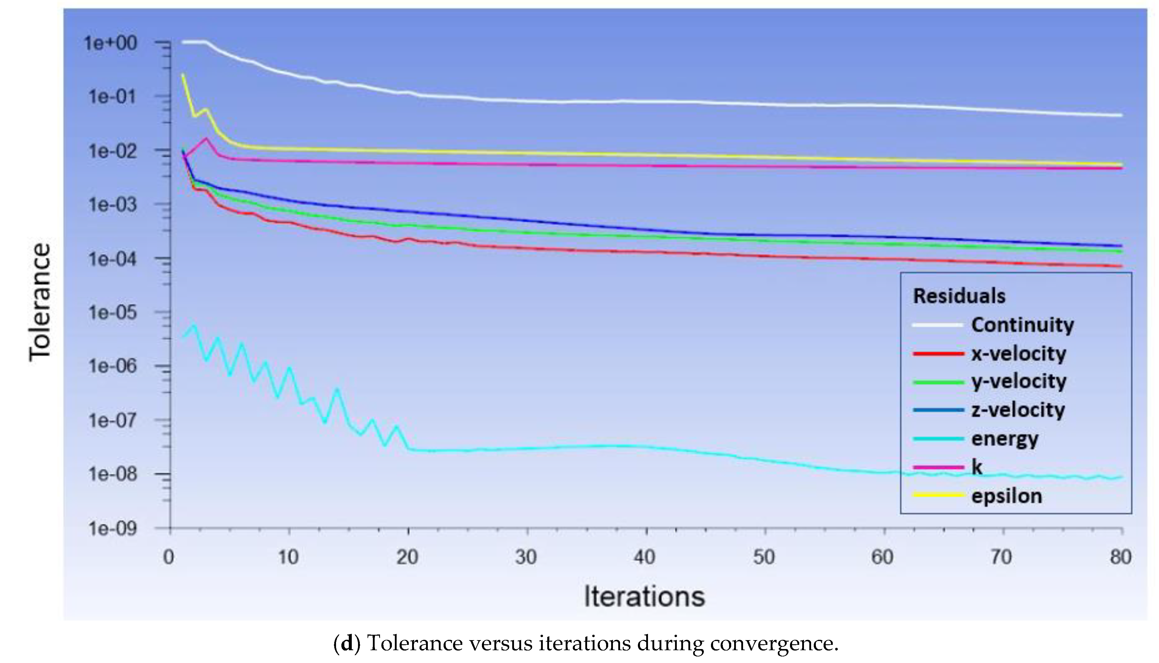
2.4. Computational Simulations

Due to the high complexity and multi-scale dimensions of the models in this study, a multi-domain meshing approach was applied with unstructured tetrahedral elements using ANSYS ICEM CFD. Convergence sensitivity analysis was conducted to ensure grid-independent predictions. The final mesh consisted of approximately 3.5 million tetrahedral elements for whole lung (Figure 1c) and approximately 0.45 million tetrahedral elements for each local bifurcation (Figure 1c). The governing airflow and momentum conservation equations were solved using the CFD package Fluent 15.0 and a user defined C program.

3. Results

The results presented were obtained based on mesh convergence from iterative solutions. The refinement error was calculated within tolerance. Basically, we increased the mesh density and analyzed the model until the results converged satisfactorily. The results of mesh refinement through convergence study, and the tolerance error with iterations during convergence are presented in Figure 2c,d, respectively. In general, the converged meshes include about 3.5 million elements for the whole lung model and about 0.43 million elements for the local airways. The converged results of velocities, pressure, and wall shear stresses for both lung model and local airways from simulations are presented below.

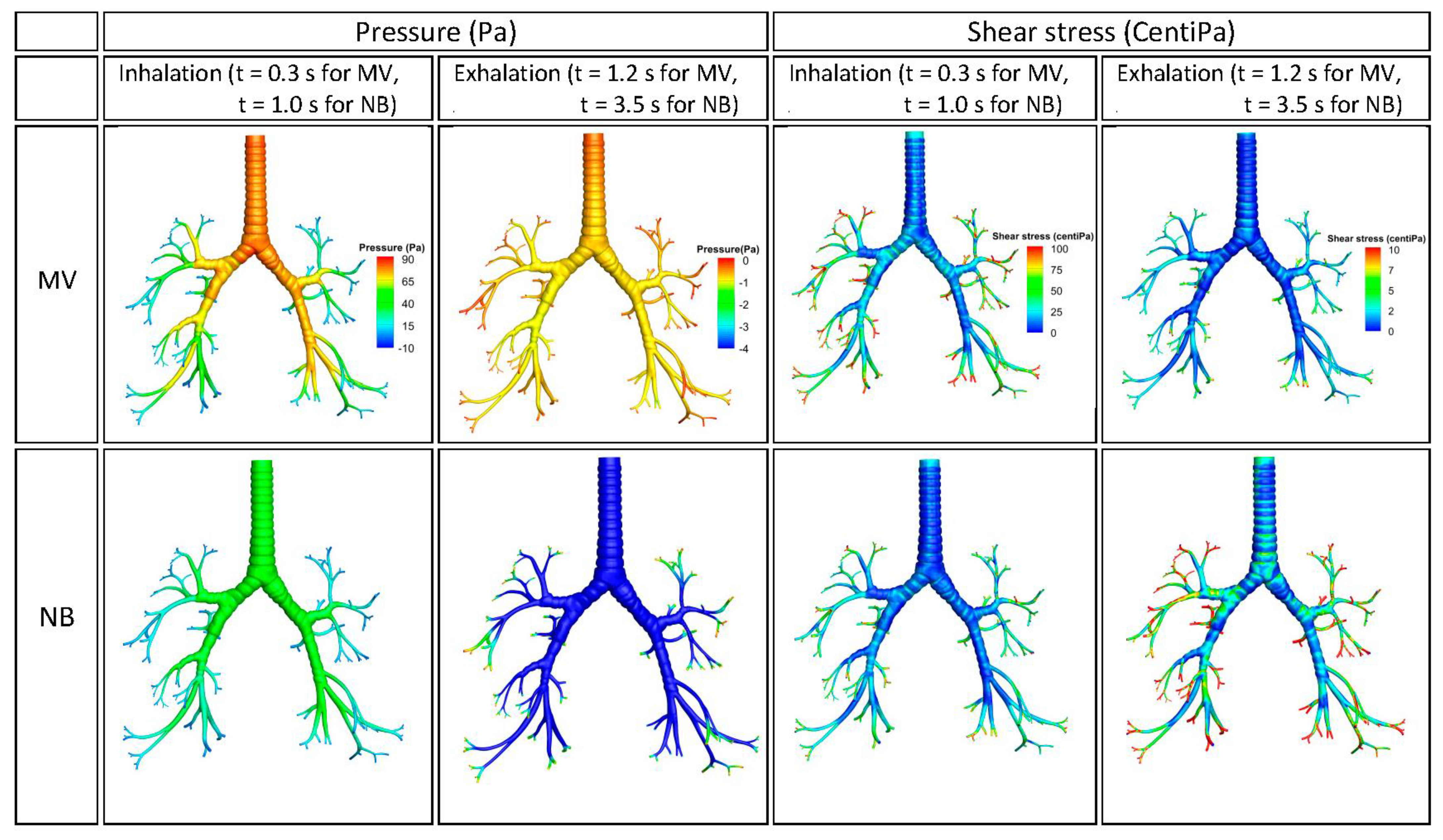
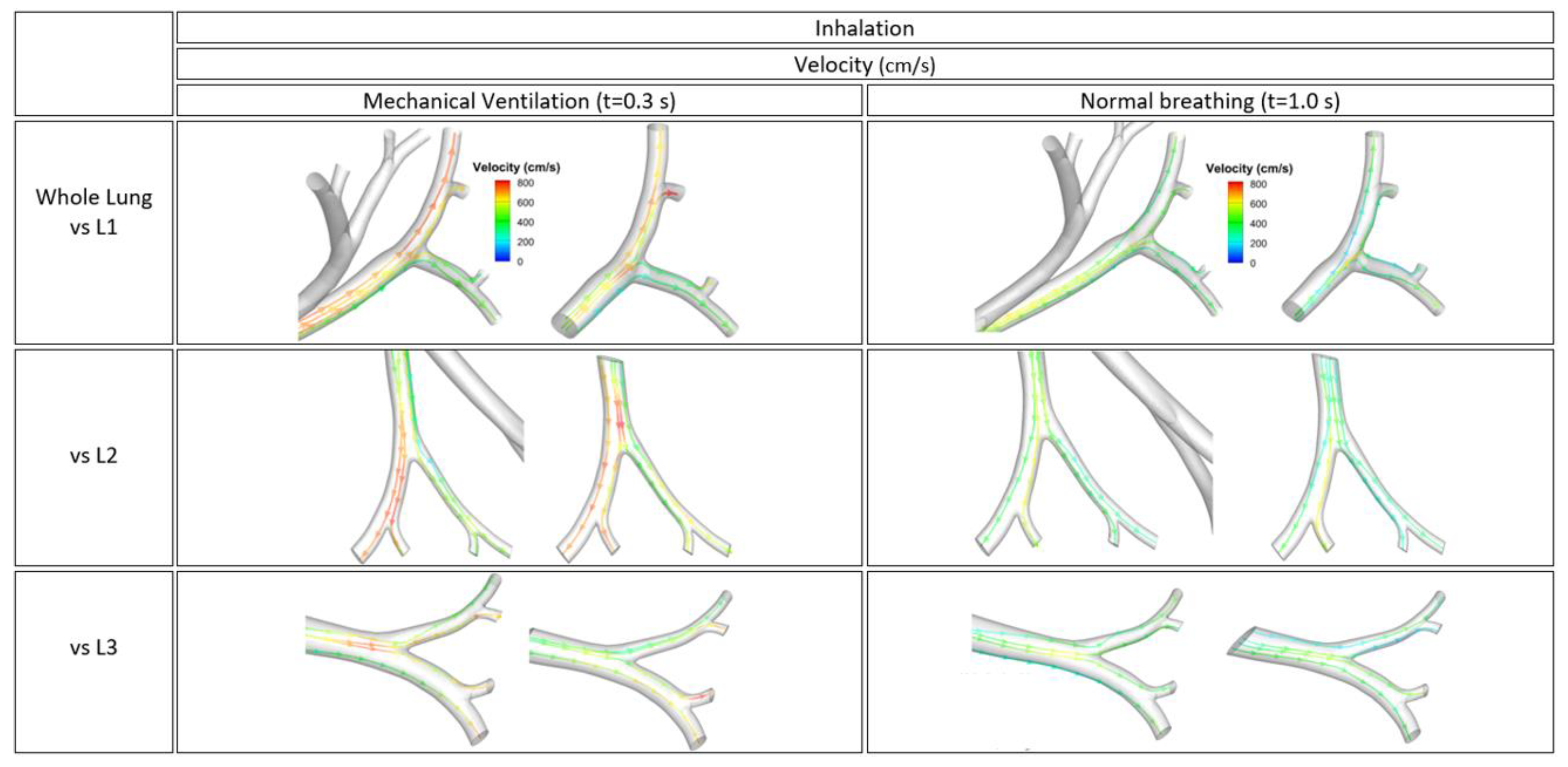
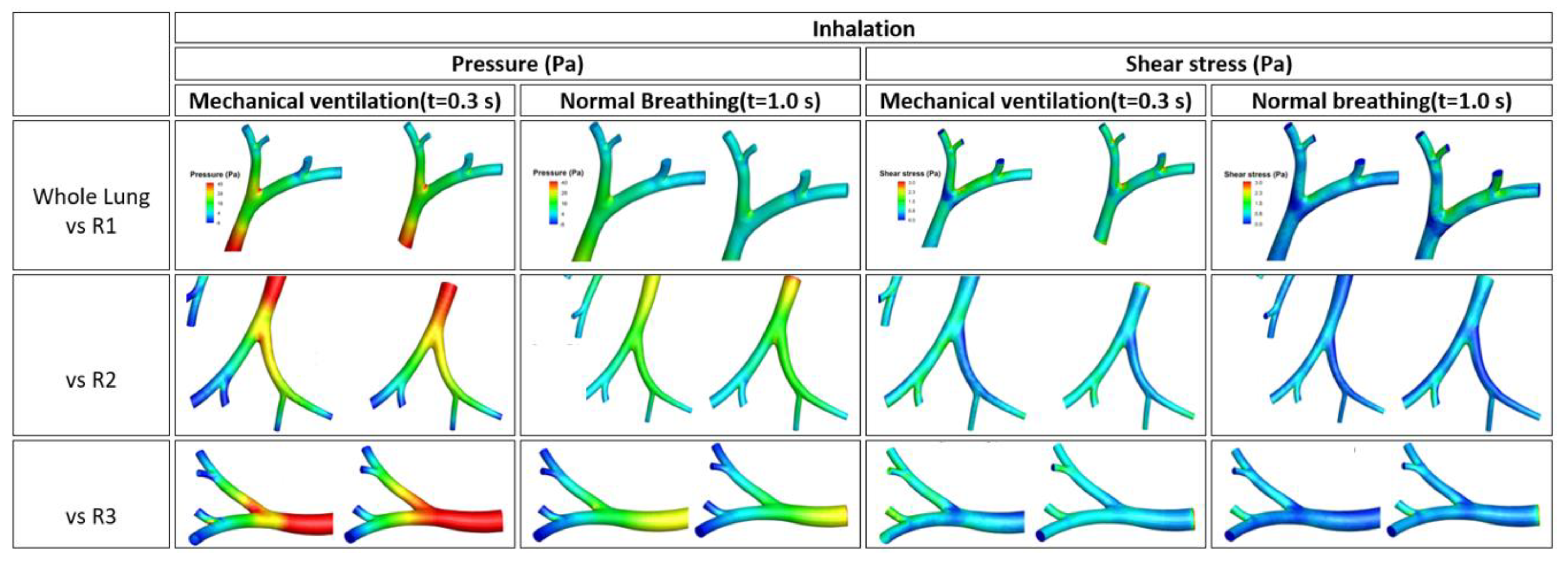
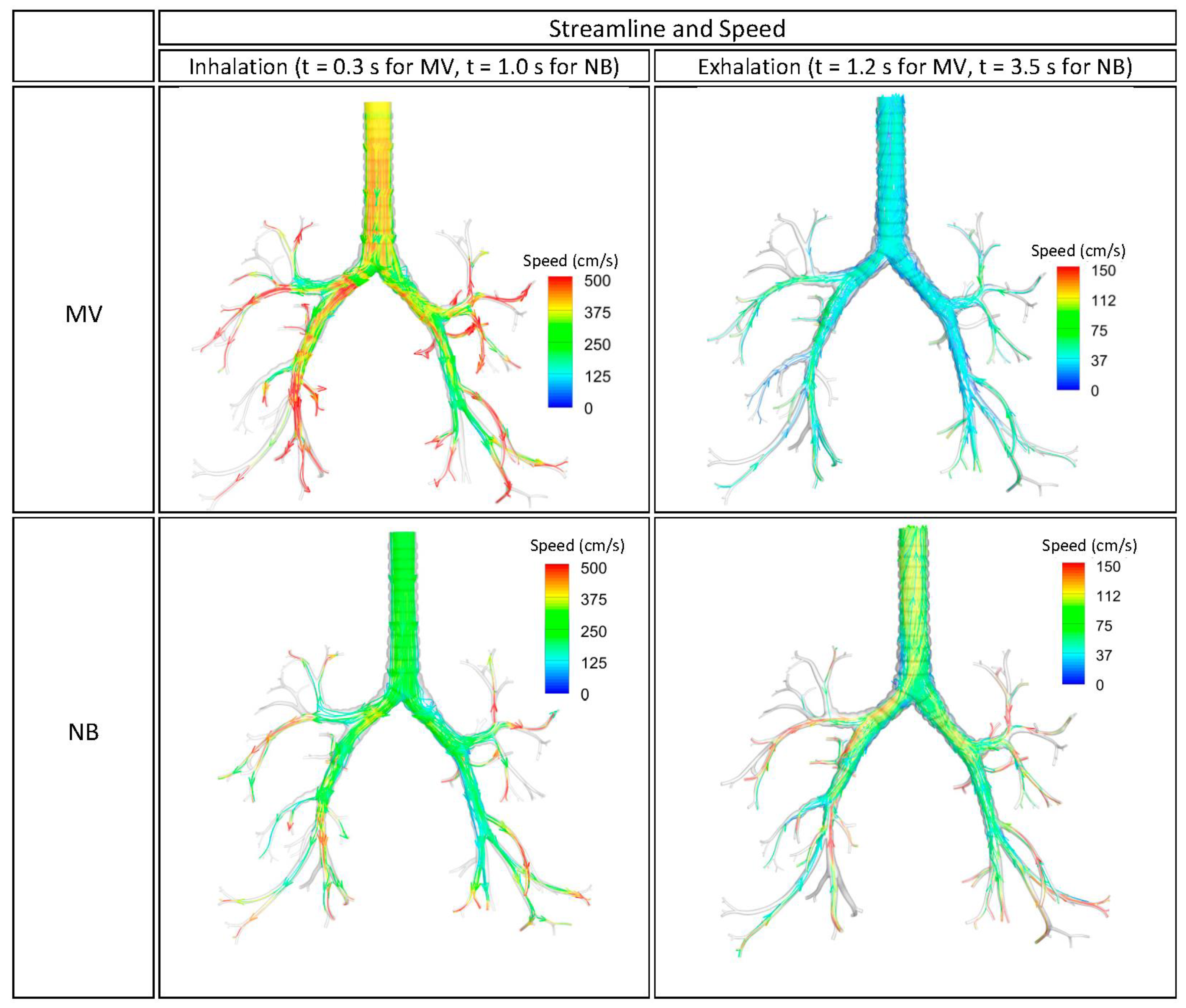
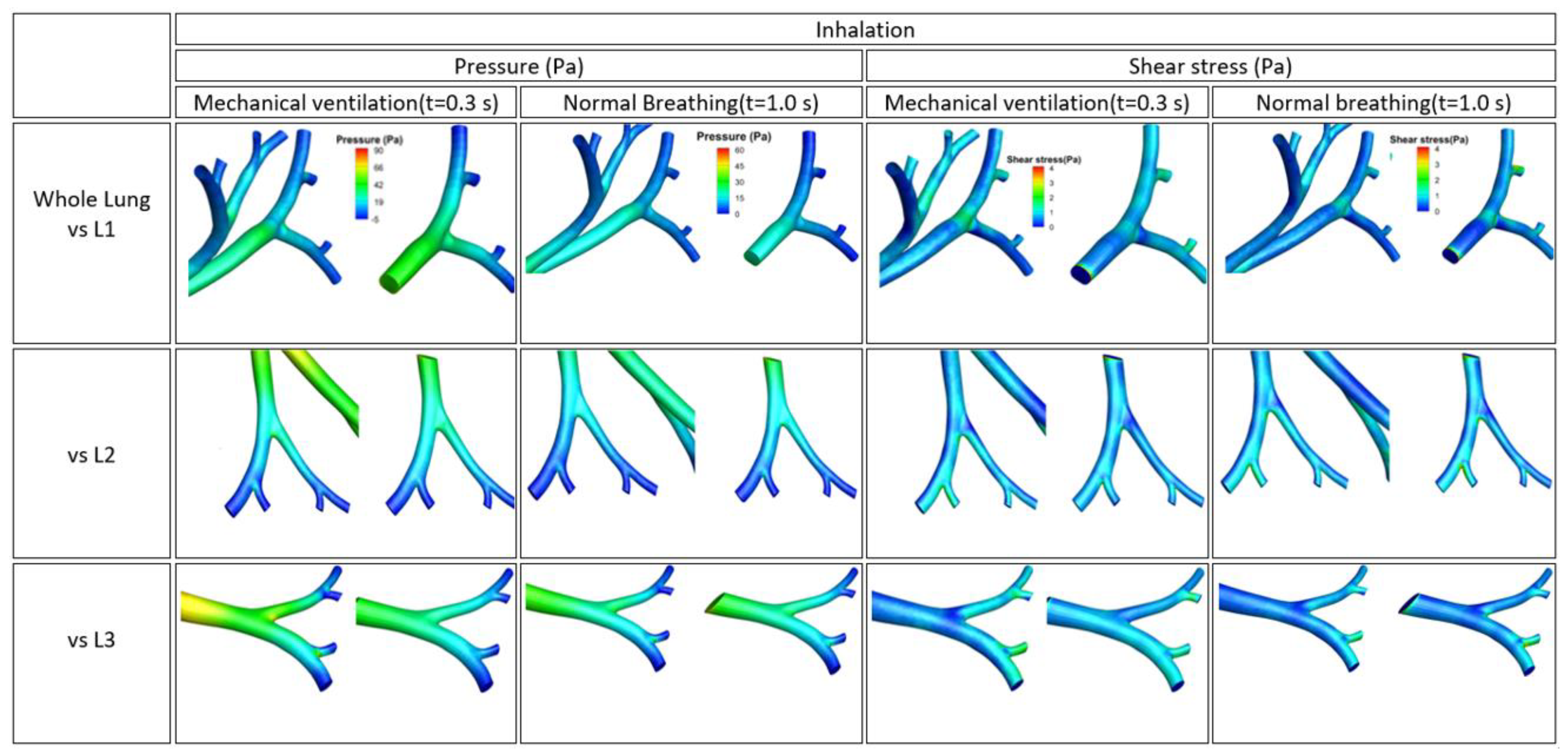
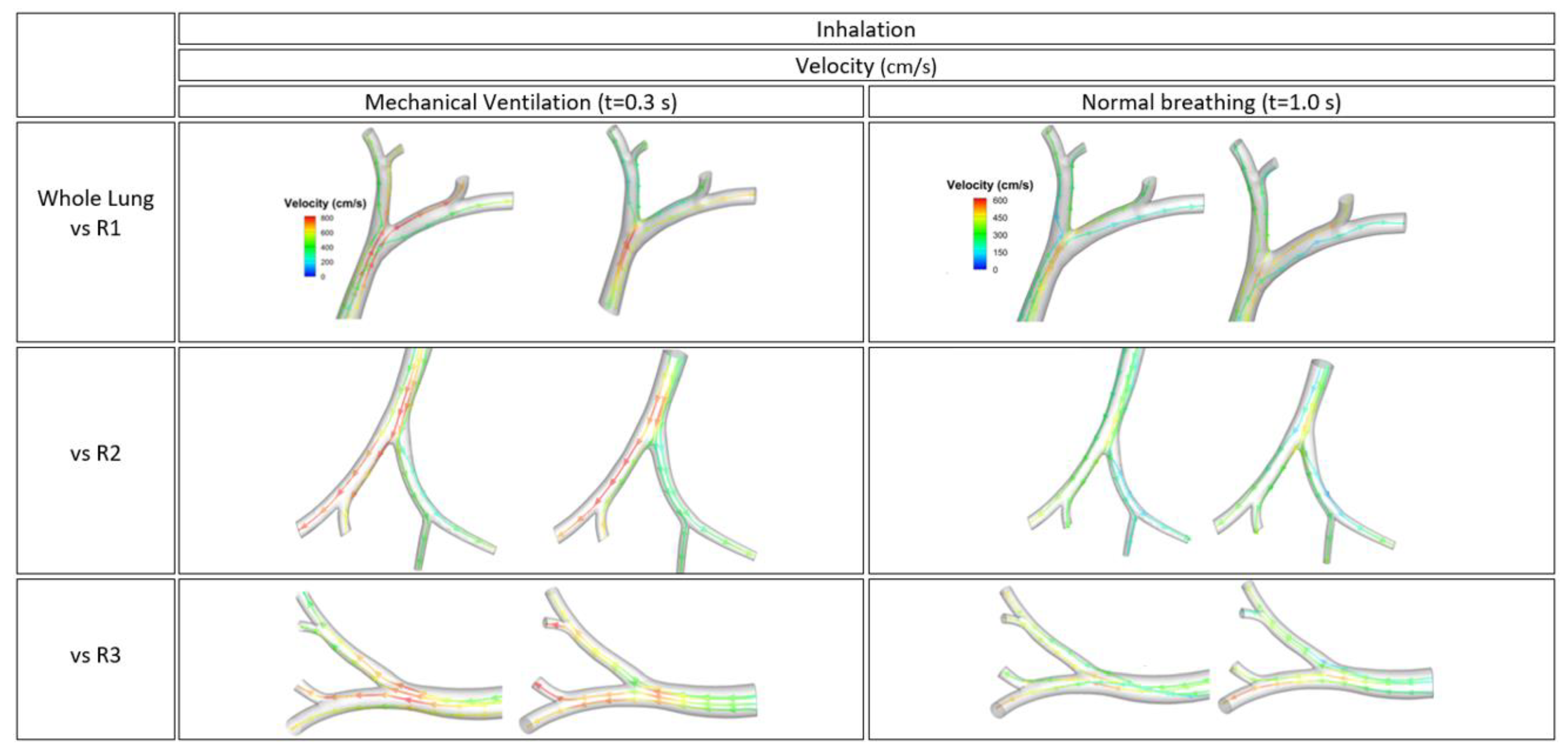
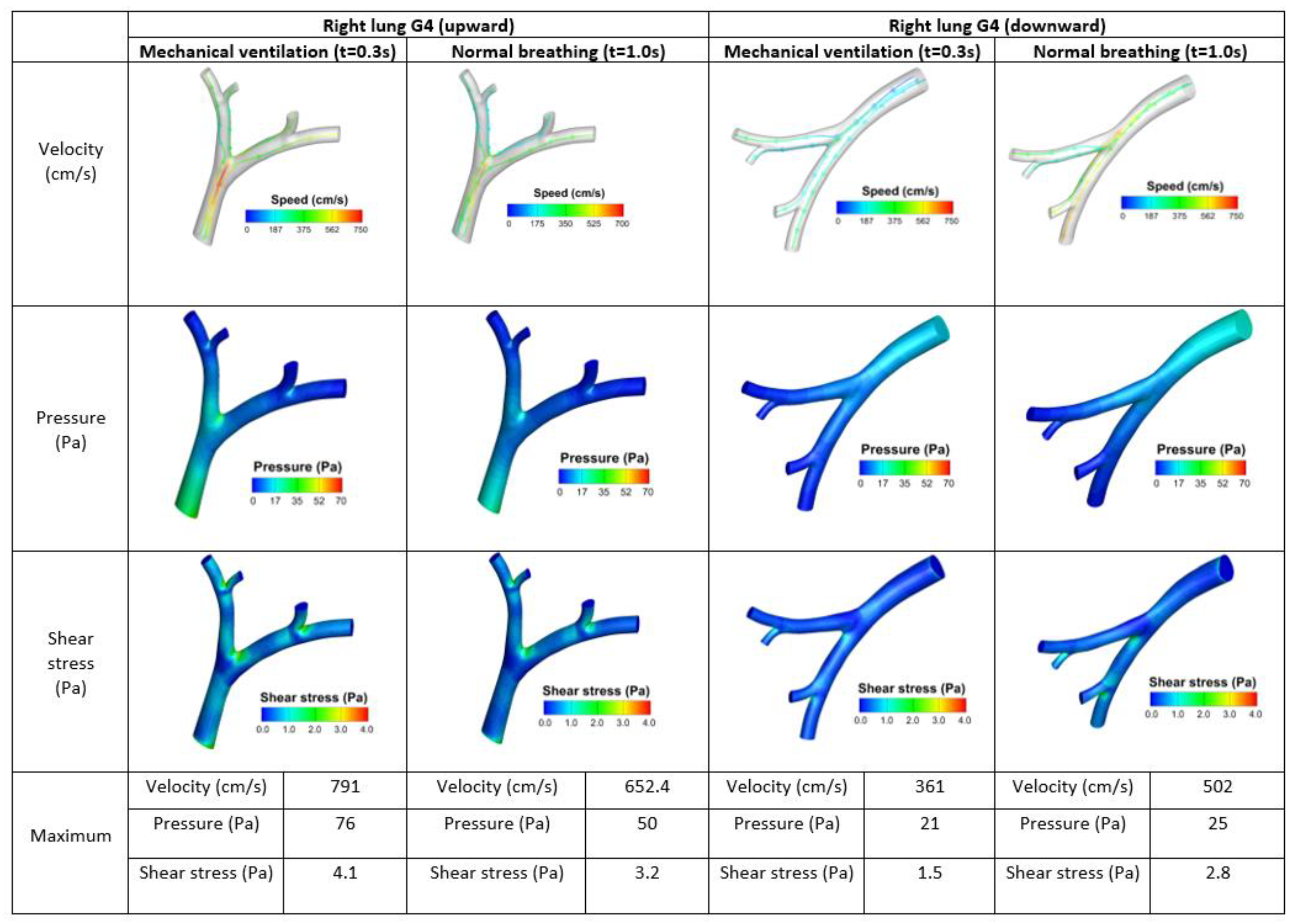
3.1. Streamline of Velocity, Contour of Pressure, and Contour Wall Shear Stress
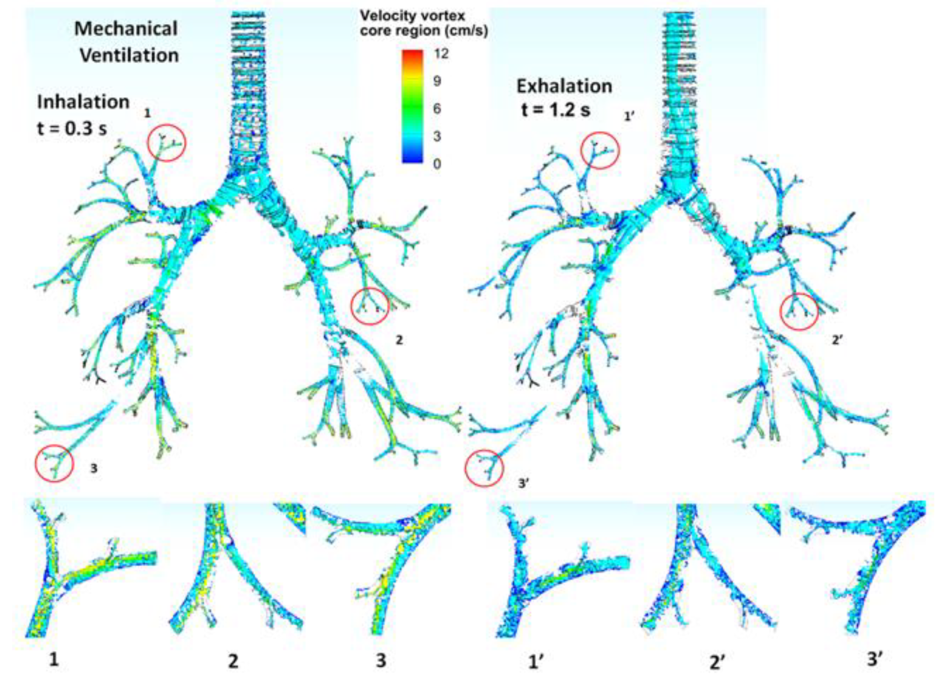
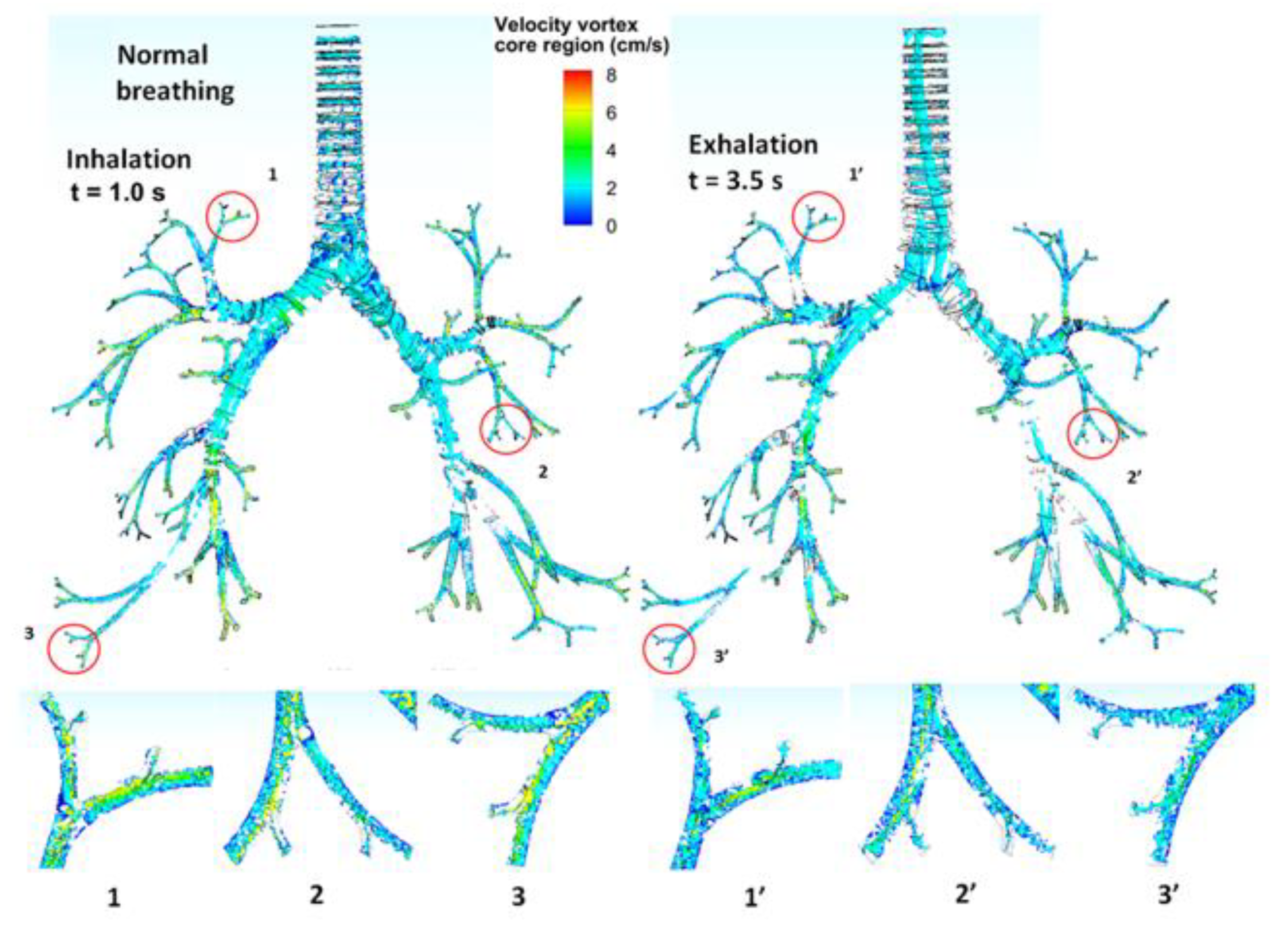
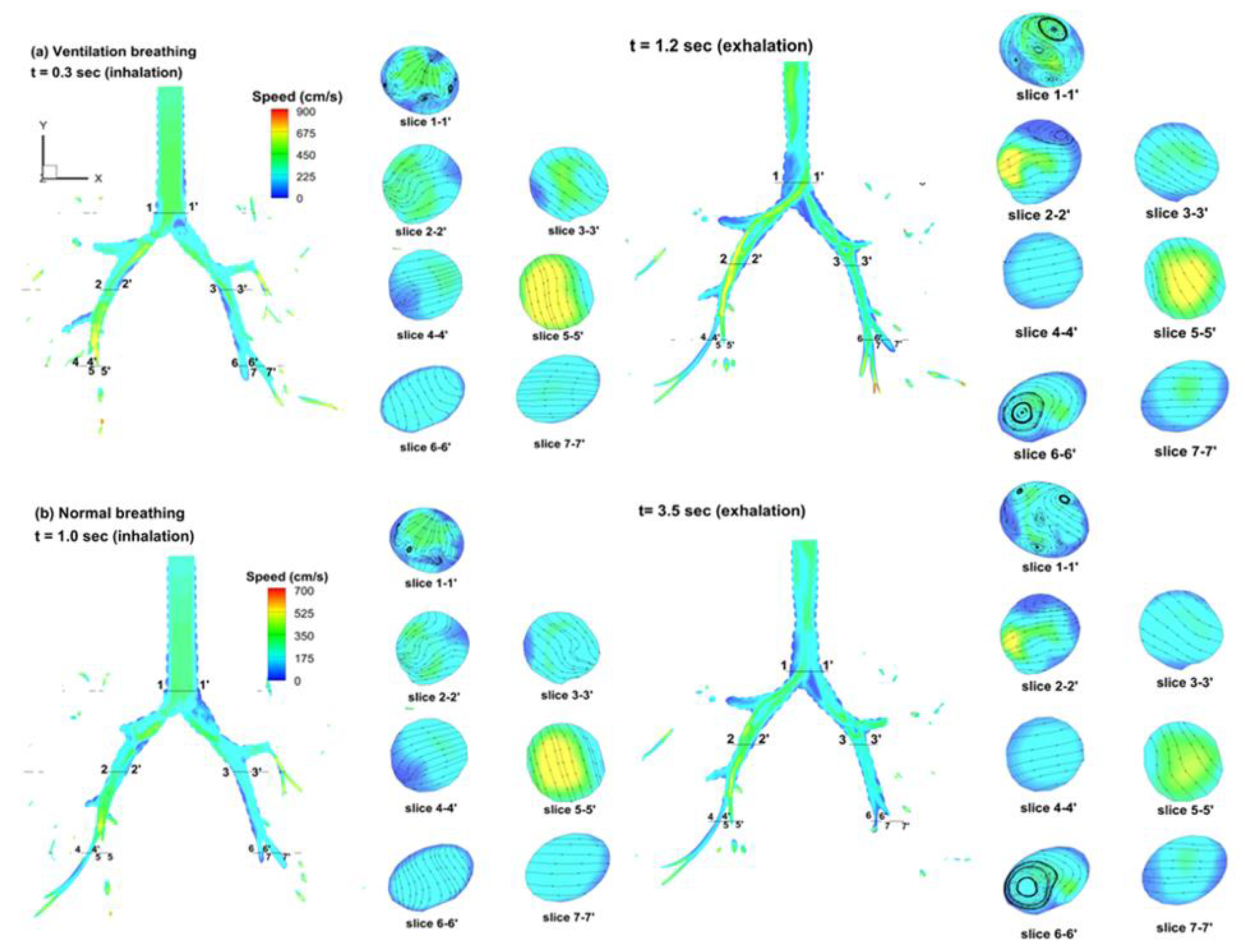
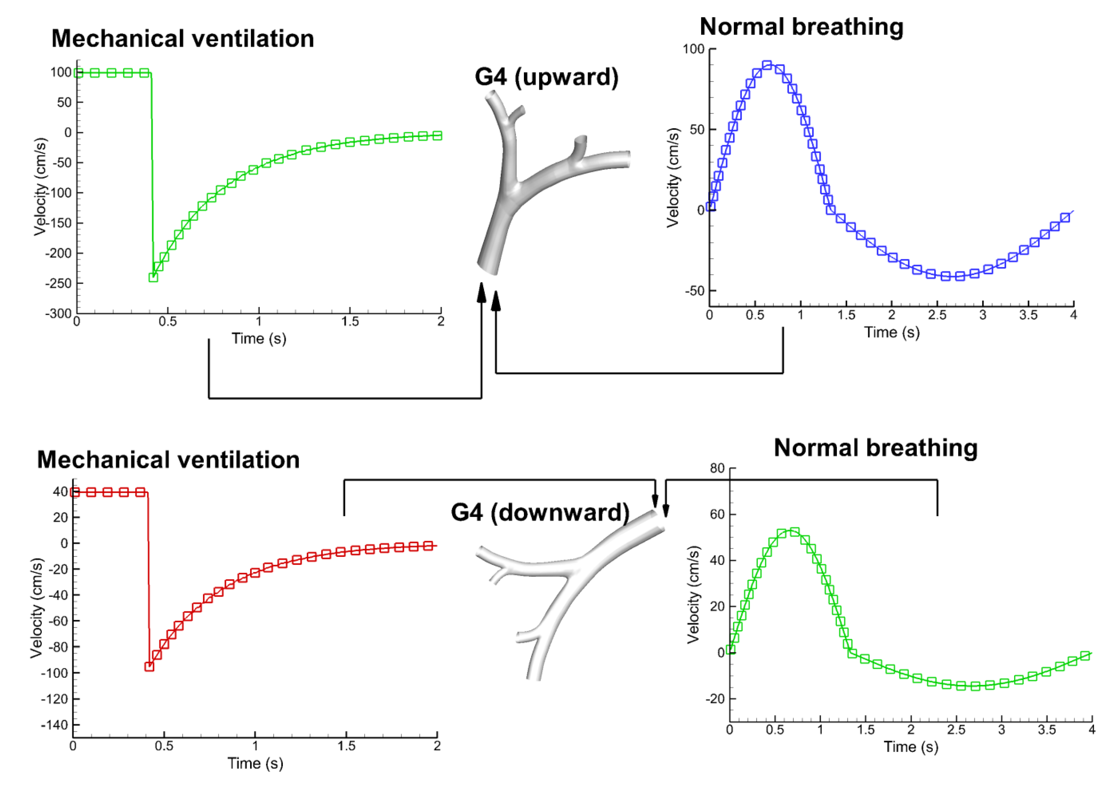
For the transient time dependent condition, the flow characteristics (velocity, pressure, and shear stress) at selected times during both inhalation and exhalation are illustrated in Figure 3 and Figure 4. During inhalation, higher speed of airflow occurred in mechanical ventilation rather than normal breathing as indicated in the bronchioles, which implies flow was at the end of the branches. In contrast, during exhalation, the speed of airflow during normal breathing was faster than during mechanical ventilation as illustrated in Figure 3.
During inhalation in mechanical ventilation, pressure is high over the TB region and bronchi, but it lowers as the stream reaches the bronchioles. However, pressure during inhalation in normal breathing is much lower than that of mechanical ventilation, as shown in Figure 4. The intensity of pressure during exhalation in mechanical ventilation is overall higher than during normal breathing, and high pressure is observed at the TB and surroundings of the bronchioles (near tips of branches) for exhalation under mechanical ventilation as indicated in Figure 4.
Surprisingly, pressure on top of trachea is zero for exhalation during mechanical ventilation and negative everywhere for exhalation during normal breathing as shown in in Figure 4. This is because the pressure drop was significant for more distant regions (lower airways) during exhalation compared with the top of the trachea. Since high speed of flow is observed on the bronchioles, most of the high shear stress occurs at the bronchioles, as shown in Figure 3. Due to higher speeds during exhalation in normal breathing compared to mechanical ventilation, shear stress is higher in normal breathing in comparison to mechanical ventilation as shown in Figure 4.

3.2. Velocity Field

The velocity field in the TB geometry is presented in Figure 5 as coronal contour profiles for an inhalation (t = 0.3 s for mechanical ventilation, t = 1.0 s for normal breathing) and exhalation (t = 0.9 s for mechanical ventilation, t = 3.5 s for normal breathing). In Figure 5a, the velocity profiles in the main trachea are maintained at approximately 450 cm/s. Compared to the trachea, lower paths of the lung have lower velocity profiles. Once the airflow closes towards the end of the bifurcations, it shifts to high velocity profiles, approximately 700–800 cm/s. The shift in the velocity profile is attributed to interactions among convective acceleration (i.e., inertial force), boundary layer effects, and centrifugal forces in the curved bifurcations. The acceleration in smaller bifurcations occurs due to the gradual airway narrowing. To illustrate the secondary motions in these regions, 2D velocity contours and stream tracers are shown in selected coronal slices. The magnitude of secondary motion in each slice is approximately 10–20% of the main flow. This secondary motion component serves to mix the inhaled or exhaled air and distribute it towards the wall. Surprisingly, stronger secondary motion is persistently observed in the trachea for inhaled ventilation and normal breathing, and depends on upstream conditions as well as the shape of the bifurcation zone.

3.3. Turbulent Vortices

Among various methods for identifying vortices, λ2-criterion has been reported to better represent the topology of vortex cores for transitional flows [18], which is the case in human respiratory flows. Physically, the λ2-criterion is formulated based on the concept of a local pressure minimum [31], to capture the region of local pressure minimum in a plane. Jeong et al. [31] defined the vortex core as a connected region with two positive eigenvalues of the pressure Hessian matrix. This affects the physical characteristics by taking the gradient of Navier–Stoke equations results, which describe fluid motion. Figure 6 and Figure 7 depict instantaneous coherent structures among the four different situations obtained using low Reynolds k-w turbulent simulations for transient breathing cycle (single period) under mechanical ventilation and normal breathing. These vortices are identified by the isosurfaces of λ2-criterion at a magnitude of 0.03 and are colored by the local airflow speed.
Vortex rings are observed to generate at the cartilage ring over the trachea and subsequently merge at the first generation stream with vortices under both mechanical ventilation and normal breathing during inhalation (see Figure 6 and Figure 7). Moreover, for locally selected bifurcations in the upper, middle, and lower parts, strong vortex rings mainly form around the interior region of local bifurcations 1, 2, and 3, as shown in Figure 6. However, during exhalation, vortex rings form differently (see Figure 6 and Figure 7)—a strong array of vortex rings is generated inside the middle passage of the trachea instead of cartilaginous rings, and vortex structures appear to be decaying at the stream to the lower lung. This is due to turbulence becoming weaker and changing to laminar flow in the bifurcations (1, 2, and 3).

3.4. Flow Characteristics of Local Bifurcations

From the whole lung model, the waveform at the specified isolated bifurcation was obtained at the inlet of the bifurcation for both mechanical ventilation and normal breathing. The results of flow characteristics including velocity, pressure, and shear stress of local bifurcations as well as whole lung are presented in Figure 8, Figure 9, Figure 10 and Figure 11. As we hypothesized, similarities were found between whole lung and isolated bifurcations in terms of velocity streamline, pressure, and shear stress contours. In whole lung vs. L1 for mechanical ventilation, velocity of the upward bronchiole was higher than that of the lower one as shown in Figure 8, and pressure decreased as the corresponding stream reached the end of the bronchiole. Shear stress was also stronger in the upward bronchiole rather than the lower one as shown in Figure 9. In whole lung vs. L3 for mechanical ventilation, the magnitude of velocity was lower overall as compared to other bifurcations, as shown in Figure 8. The shear stresses were stronger around the end of the branches, as shown in Figure 9.
In contrast, a lower speed in the entire region of bifurcations was observed under normal breathing (see Figure 8) as compared to all the cases (whole lung vs. L1, L2, and L3) under mechanical ventilation. The similarities in flow characteristics between whole lung vs. R1, R2, and R3 are shown in Figure 10 and Figure 11, respectively. Under mechanical ventilation, the whole lung vs. R1 and R3 bifurcations, the magnitude of velocity is quite similar on the left and right sides of the bronchiole as shown in Figure 10. However, for the whole lung vs. R2 bifurcation, the left bronchiole has a higher speed of airflow than the right one, but shear stress at the left side of the bronchiole in whole lung vs. R2 is stronger than that for the right side as shown in Figure 11. Under normal breathing, for the whole lung vs. R3, the lower side of the bronchiole has a faster velocity stream trace than the upward bronchiole.
To verify the airflow similarity between whole lung models versus local bifurcations, the ratio of pressure and shear stress at 9 selected points (all the nodes in the bifurcation path) is presented in Table 2. The difference in similarity is in the range of 3–6%, and the maximum difference was 9% and it occurred at point 8 of left local bifurcation L3 (Figure 12 and Table 2). This finding shows that the present approach will help to reduce the computation time when analyzing whole lung for clinical applications.
Figure 13 and Figure 14 show the differences between bifurcations for the same side (right lung), the same generation (fourth), and different regions (upward and downward) of the local bifurcations instead of whole lung under mechanical ventilation and normal breathing conditions. It can be seen from Figure 13 that the upward bifurcation shows a higher velocity magnitude under mechanical ventilation. Moreover, the velocity streamtrace, pressure, and shear stress, are all stronger as shown in Figure 14. Under normal breathing, similar trends to that seen under the mechanical ventilation were observed.

4. Discussion

We hypothesized that breathing under mechanical ventilation would be significantly different from normal breathing due to differences in air flow pattern and magnitude of tidal volume. This hypothesis was investigated through the CFD simulation of airflow in the human lung respiratory tract. No slip boundary conditions and steady static pressure were assumed, and air was modeled as an incompressible Newtonian fluid with constant density and viscosity, consistent with previous studies [1,16,24,32]. Both mechanical ventilation and normal breathing conditions were simulated by user-defined function under transient flow conditions in a realistic TB model. The bifurcating pattern of the TB model is typically asymmetric, with daughter branches from the same parent often differing in both diameter and length. Furthermore, the spatial orientations of the bifurcating branches are variable, resulting in an architecture that is highly out-of-plane. Specific velocity inlet and pressure outlet boundary conditions were considered [13,19,33,34]. The inlet velocity or flow rate was determined based on past studies [24,35,36,37].
Flow characteristics in mechanical ventilation and normal breathing followed an expected pattern as illustrated in Figure 3 and Figure 4. There was a low-pressure field at the bronchioles during inhalation in mechanical ventilation and in normal breathing. The velocity field (Figure 3 and Figure 4) and the pressure field were high at the bronchioles during exhalation in mechanical ventilation and normal breathing (Figure 3 and Figure 4). These results imply that as air from the inlet is inhaled and flows through the TB region, a smaller amount of air might reach the outlets. The trachea region became more turbulent as seen in slice 1-1′ and the vortex region as shown in Figure 6 and Figure 7.
Marked differences between mechanical ventilation (Figure 6) and normal breathing (Figure 7) were observed in terms of vortices generation that may be due to the difference in flow rate and Reynolds number. Shear stress at the airway wall indicated that the forces were exerted tangentially to the inner luminal wall of the airway. Airflow was accelerated, leading to turbulence that disrupted the boundary layer and resulted in high wall shear stress. As large wall shear stress variations in blood vessels might increase the risk of arteriosclerosis, the high shear stress at the stenotic site would correlate with the trauma of the airway mucosa and an inflammatory response [22].
We also verified similarities in terms of flow characteristics (Figure 8, Figure 9, Figure 10 and Figure 11 and Table 2), such as velocity, pressure and shear stress, between local bifurcations and the whole lung. Such a similarity means that airway flow is essentially influenced by local geometrical conditions with little influence from the generations located upstream from the ones considered. The results shown are not identical because the cutting of the whole lung to match isolated local bifurcations was not quite even. This caused slight differences in velocity, pressure, and shear stress contours and values. For this verification, we used two isolated local bifurcations of the same generation (fourth), same side (right), and different regions (upward and downward). The results in terms of both contours and maximum values are shown in in Figure 14. The upward bifurcation showed higher flow characteristics in terms of velocity, pressure, and shear stress for both mechanical ventilation and normal breathing. This might have occurred because the airflow inlet for the upward bifurcation is smaller than that for the downward bifurcation, which makes airflow velocity faster. Moreover, the total outlet area of the upward bifurcation is larger than that for the downward bifurcation, so the tidal volume of the upward bifurcation is larger than the downward one. Concerning differences in regional flow distribution, it is surprising that the upward bifurcation has a higher velocity magnitude than the downward one because, due to convective inertia, fluid tends to go straight.
In conclusion, the differences in flow characteristic between mechanical ventilation and normal breathing are significant in whole lung G9 geometrical airway during inhalation and exhalation. A higher speed of airflow was observed for inhalation under mechanical ventilation than normal breathing and lower than normal breathing was observed for exhalation. Interestingly, there was no difference for pressure during exhalation between mechanical ventilation and normal breathing. The similarity of flow characteristics between whole lung and isolated bifurcations also indicates that the generation effect is significant.
Limitations of this study include use of rigid walls in our model, limited amount of test cases for local bifurcations, and limited whole lung TB geometry of G9 (real size is G23 including alveolar sacs), as well as the fact that we also assumed the boundary condition of outlet as simple (outlet pressure = 0 Pa). This should be considered as a realistic condition in future studies. We plan to address these limitations by examining the wall and tissue effect through a fluid structure interaction (FSI) simulation and simulating the whole lung including alveolar sacs (G23) to investigate flow patterns and characteristics inside alveolar sacs. The elasticity and vibration of the walls of the lung and airway effects are not included in this study, and can be investigated in future studies.

Author Contributions

Conceptualization, R.M.P.; methodology, R.M.P., J.K.; validation, J.K.; investigation, R.M.P. and J.K.; writing—original draft preparation, J.K.; writing—review and editing, R.M.P.; supervision, R.M.P.; project administration, R.M.P.; funding acquisition, R.M.P. All authors have read and agreed to the published version of the manuscript.

Funding

This research was funded by the US National Science Foundation (CMMI–1430379) and US National Institutes of Health (R01AG041823).

Institutional Review Board Statement

Not applicable.

Informed Consent Statement

Not applicable.

Data Availability Statement

No supporting data.

Acknowledgments

The authors thank the NSF 1430379 and NIH (R01AG041823) for their support. Thanks also go to Jinxiang Xi for providing the whole lung model and to Raghu Arambakam for help with the user defined routine for inputting into the model. Thanks to Angela Reynolds and Rebecca Heise of Virginia Commonwealth University for their help and support.

Conflicts of Interest

The authors declare no conflict of interest.

References

  1. Kim, J.; Xi, J. Dynamic growth and deposition of hygroscopic aerosols in the nasal airway of a 5-year-old child. Int. J. Numer. Meth. Eng. 2013, 29, 17–39. [Google Scholar] [CrossRef] [PubMed]
  2. Si, X.; Xi, J.; Kim, J.; Zhou, Y.; Zhong, H. Modeling of release position and ventilation effects on olfactory aerosol drug delivery. Respir. Physiol. Neurobiol. 2013, 186, 22–32. [Google Scholar] [CrossRef] [PubMed]
  3. Xi, J.; Berlinski, A.; Zhou, Y.; Greenberg, B.; Ou, X. Breathing resistance and ultrafine particle deposition in nasal-laryngeal airways of a newborn, an infant, a child, and an adult. Ann. Biomed. Eng. 2012, 40, 2579–2595. [Google Scholar] [CrossRef] [PubMed]
  4. Zhao, K.; Scherer, P.W.; Hajiloo, S.A.; Dalton, P. Effect of anatomy on human nasal air flow and odorant transport patterns: Implications for olfaction. Chem. Senses 2004, 29, 365–379. [Google Scholar] [CrossRef]
  5. Heyder, J.; Gebhart, J.; Rudolf, G.; Schiller, C.F.; Stahlhofen, W. Deposition of particles in the human respiratory tract in the size range of 0.005–15 μm. J. Aerosol Sci. 1986, 17, 811–825. [Google Scholar] [CrossRef]
  6. Jaques, P.A.; Kim, C. Measurement of total lung deposition of inhaled ultrafine particles in healthy men and women. Inhal. Toxicol. 2000, 12, 715–731. [Google Scholar]
  7. Kim, C.; Jaques, P. Analysis of total respiratory deposition of inhaled ultrafine particles in adult subjects at various breathing patterns. Aerosol Sci. Technol. 2004, 38, 525–540. [Google Scholar] [CrossRef] [Green Version]
  8. Proetz, A. Air currents in the upper respiratory tract and their clinical importance. Ann. Otol. Rhinol. Laryngol. 1951, 60, 439–467. [Google Scholar] [CrossRef]
  9. Schroter, R.C.; Sudlow, M. Flow patterns in models of the human bronchial airways. Respir. Physiol. 1969, 7, 341–355. [Google Scholar] [CrossRef]
  10. Morawska, L.; Hofmann, W.; Hitchins-Loveday, J.; Swanson, C.; Mengersen, K. Experimental study of the deposition of combustion aerosols in the human respiratory tract. J. Aerosol Sci. 2005, 36, 939–957. [Google Scholar] [CrossRef] [Green Version]
  11. Stahlhofen, W.; Rudolf, G.; James, A.C. Intercomparison of experimental regional aerosol deposition data. J. Aerosol Med. 1989, 2, 285–308. [Google Scholar] [CrossRef]
  12. Chang, H.; El, O. A model study of flow dynamics in human central airways. Respir. Physiol. 1982, 49, 75–95. [Google Scholar] [CrossRef]
  13. Horsfield, K.; Gladys, D.; Olson, D.; Finlay, G.; Cumming, G. Models of the human bronchial tree. J. Appl. Physiol. 1971, 31, 207–217. [Google Scholar] [CrossRef]
  14. Van, C.; Hirsch, C.; Paiva, M. Anatomically based three-dimensional model of airways to simulate flow and particle transport using computational fluid dynamics. J. Appl. Physiol. 2005, 98, 970–980. [Google Scholar]
  15. Heenan, A.F.; Matida, E.; Pollard, A.; Finlay, W.H. Experimental measurements and computational modeling of the flow field in an idealized human oropharynx. Exp. Fluids 2003, 35, 70–84. [Google Scholar] [CrossRef]
  16. Xi, J.; Kim, J.; Si, X. Transport and absorption of anesthetic vapors in a mouth-lung model extending to G9 bronchioles. Int. J. Anesthesiol. Res. 2013, 1, 6–19. [Google Scholar] [CrossRef]
  17. Isabey, D.; Chang, H. Steady and unsteady pressure-flow relationships in central airways. J. Appl. Physiol. 1981, 51, 1338–1348. [Google Scholar] [CrossRef]
  18. Yeh, H.; Schum, G. Models of human lung airways and their application to inhaled particle deposition. J. Math. Biol. 1980, 42, 461–480. [Google Scholar] [CrossRef]
  19. Elad, D.; Wolf, M.; Keck, T. Air-conditioning in the human nasal cavity. Respir. Physiol. Neurobiol. 2008, 163, 121–127. [Google Scholar] [CrossRef]
  20. Hörschler, I.; Meinke, M.; Schröder, W. Numerical simulation of the flow field in a model of the nasal cavity. J. Comput. Fluids 2003, 32, 39–45. [Google Scholar] [CrossRef]
  21. Hammersley, J.; Olson, D. Physical models of the smaller pulmonary airways. J. Appl. Physiol. 1992, 72, 2402–2414. [Google Scholar] [CrossRef]
  22. Wilcox, D. Turbulence Modeling for CFD, 2nd ed.; DCW Industries: La Canada, CA, USA, 1998. [Google Scholar]
  23. Xi, J.; Longest, P. Evaluation of a drift flux model for simulating submicrometer aerosol dynamics in human upper tracheobronchial airways. Ann. Biomed. Engin. 2007, 36, 1714–1734. [Google Scholar] [CrossRef]
  24. Keyhani, K.; Scherer, P.; Mozell, M. Numerical simulation of airflow in the human nasal cavity. J. Biomed. Engin. 1995, 117, 429–441. [Google Scholar] [CrossRef]
  25. Keyhani, K.; Scherer, P.; Mozell, M. A numerical model of nasal odorant transport for the analysis of human olfaction. J. Theor Biol. 1997, 186, 279–301. [Google Scholar] [CrossRef]
  26. Lindemann, J.; Leiacker, R.; Rettinger, G.; Keck, T. Nasal mucosal temperature during respiration. Clin. Otolaryngol. 2002, 27, 135–139. [Google Scholar] [CrossRef]
  27. Lindemann, J.; Keck, T.; Wiesmiller, K.; Sander, B.; Brambs, H.; Rettinger, G.; Pless, D. A numerical simulation of intranasal air temperature during inspiration. Laryngoscope 2004, 114, 1037–1041. [Google Scholar] [CrossRef]
  28. Lindemann, J.; Keck, T.; Wiesmiller, K.; Rettinger, G.; Brambs, H.; Pless, D. Numerical simulation of intranasal air flow and temperature after resection of the turbinates. Rhinology 2005, 43, 24–28. [Google Scholar]
  29. Heistracher, T.; Hofmann, W. Physiologically realistic models of bronchial airway bifurcations. J. Aerosol Sci. 1995, 26, 497–509. [Google Scholar] [CrossRef]
  30. Cohen, B.; Sussman, R.; Lippmann, M. Ultrafine particle deposition in a human tracheobronchial cast. Aerosol Sci. Technol. 1990, 12, 1082–1093. [Google Scholar] [CrossRef]
  31. Jeong, J.; Hussain, F. On the identification of a vortex. J. Fluid Mech. 1995, 285, 69–94. [Google Scholar] [CrossRef]
  32. Lee, J.; Yang, N.; Kim, S.; Chung, S. Unsteady flow characteristics through a human nasal airway. Respir. Physiol. Neurobiol. 2010, 172, 136–146. [Google Scholar] [CrossRef] [PubMed]
  33. Liu, Y.; Matida, A.; Gu, J.; Johnson, M. Numerical simulation of aerosol deposition in a 3-D human nasal cavity using RANS, RANS/EIM, and LES. J. Aerosol Sci. 2007, 38, 683–700. [Google Scholar] [CrossRef]
  34. Perzl, M.; Schultz, H.; Parezke, H.; Englmeier, K.; Heyder, J. Reconstruction of the lung geometry for the simulation of aerosol transport. J. Aerosol Med. 1996, 9, 409–418. [Google Scholar] [CrossRef]
  35. Vial, L.; Perchet, D.; Fodil, R.; Caillibotte, G.; Fetita, C.; Preteux, F. Airflow modeling of steady inspiration in two realistic proximal airway trees reconstructed from human thoracic tomodensitometric images. Comput. Methods Biomech. Biomed. Eng. 2005, 8, 267–277. [Google Scholar] [CrossRef]
  36. Xi, J.; Longest, P.; Martonen, T. Effects of the laryngeal jet on nano-and microparticle transport and deposition in an approximate model of the upper tracheobronchial airways. J. Appl. Physiol. 2008, 104, 1761–1777. [Google Scholar] [CrossRef]
  37. Kleinstreuer, C.; Zhang, Z. Airflow and particle transport in the human respiratory system. J. Fluid Mech. 2010, 42, 301–334. [Google Scholar] [CrossRef]
Figure 1. Imaged-based realistic trachea whole lung airway model: (a) breathing waveform of flow rate for mechanical ventilation (MV) and normal breathing (NB); (b) surface geometry model; and (c) computational mesh. The mesh contains proximately 3.5 million unstructured tetrahedral elements.
Fluids 06 00388 g001
Figure 2. Imaged-based realistic isolated bifurcation airway model: (a) surface geometry model and breathing waveform of flow rate for mechanical ventilation (MV) and normal breathing (NB); (b) computational mesh. The mesh contains proximately 0.45 million unstructured tetrahedral elements for each bifurcation; (c) convergence study through increasing mesh density; and (d) tolerance error with iterations plot during convergence.
Fluids 06 00388 g002aFluids 06 00388 g002b
Figure 3. Comparison of airflow of stream trace and speed for the MV and NB. Comparison during inhalation (t = 0.3 s for MV, t = 1.0 s for NB) and exhalation (t = 1.2 s for MV, t = 3.5 s for NB).
Fluids 06 00388 g003
Figure 4. Comparison of airflow of pressure and shear stress for the MV and NB. The comparison was during inhalation (t = 0.3 s for MV, t = 1.0 s for NB) and exhalation (t = 1.2 s for MV, t = 3.5 s for NB).
Fluids 06 00388 g004
Figure 5. Comparison of velocity field using sagittal and cross-sectional view: instantaneous mid-plane contours of velocity magnitude, and in-plane streamlines of secondary motion in the trachea, left and right lung under transient conditions (a) t = 0.3 s, t = 1.0 s for mechanical ventilation, and (b) t = 0.9 s, t = 3.5 s for normal breathing).
Fluids 06 00388 g005
Figure 6. Turbulent spot prediction for Mechanical Ventilation: Vortices through iso-surface during inhalation (t = 0.3 s) and exhalation (t = 1.2 s) for mechanical ventilation with highlighted local bifurcations. Selected local bifurcations are two from right lung and one from left lung.
Fluids 06 00388 g006
Figure 7. Turbulent spot prediction for Normal Breathing: Vortices through iso-surface during inhalation (t = 1.0 s) and exhalation (t = 3.5 s) for normal breathing with highlighted local bifurcations. Selected local bifurcations are two from right lung and one from left lung.
Fluids 06 00388 g007
Figure 8. Comparison of airflow velocity for left bifurcations of whole lung and isolated local bifurcations (L1, L2, and L3). The plots are for the MV and NB during inhalation at t = 0.3 s, t = 1.0 s, respectively.
Fluids 06 00388 g008
Figure 9. Comparison of pressure and shear stress for left bifurcations of whole lung and isolated local bifurcations (L1, L2, and L3). The plots are for the MV and NB during inhalation at t = 0.3 s, t = 1.0 s, respectively.
Fluids 06 00388 g009
Figure 10. Comparison of airflow velocity for right bifurcations of whole lung and isolated local bifurcations (R1, R2, and R3). The plots are for the MV and NB during inhalation at t = 0.3 s, t = 1.0 s, respectively.
Fluids 06 00388 g010
Figure 11. Comparison of pressure and shear stress for right bifurcations of whole lung and isolated local bifurcations (R1, R2, and R3). The plots are for the MV and NB during inhalation at t = 0.3 s, t = 1.0 s, respectively.
Fluids 06 00388 g011
Figure 12. Selected points of the whole lung and local bifurcation.
Fluids 06 00388 g012
Figure 13. Comparison of bifurcation waveforms. The waveforms used for MV and the NB at the upward bifurcation (top) and downward (bottom) bifurcation for fourth generation in the right lung.
Fluids 06 00388 g013
Figure 14. Comparison of simulations for the upward and downward G4 bifurcation. Comparison of the maximum velocity, pressure, shear stress, values at the upward and downward fourth generation local bifurcations of the right lung for MV and the NB.
Fluids 06 00388 g014
Table 1. Respiratory parameters of whole lung model.
Tracheobronchial Whole Lung (G9)
Tidal volume (mL)Ventilation420
Normal700
Breathing frequency (Hz)Ventilation0.5
Normal0.25
I:E ratioVentilation1:4
Normal1:2
Inhalation (s)Ventilation0.4
Normal1.33
Table 2. Ratio, α and β of pressure and shear stress at selected 9 points in Figure 12 in whole lung (left and right) and isolated local bifurcations (L1, L2, L3, R1, R2, R3). Pn(α) = pressure of selected point in whole lung/pressure of selected point in local bifurcation, n = 1,2,3,4,5,6,7,8,9), Sn(β) = shear stress of selected point in whole lung/shear stress of selected point in local bifurcation, n = 1,2,3,4,5,6,7,8,9).
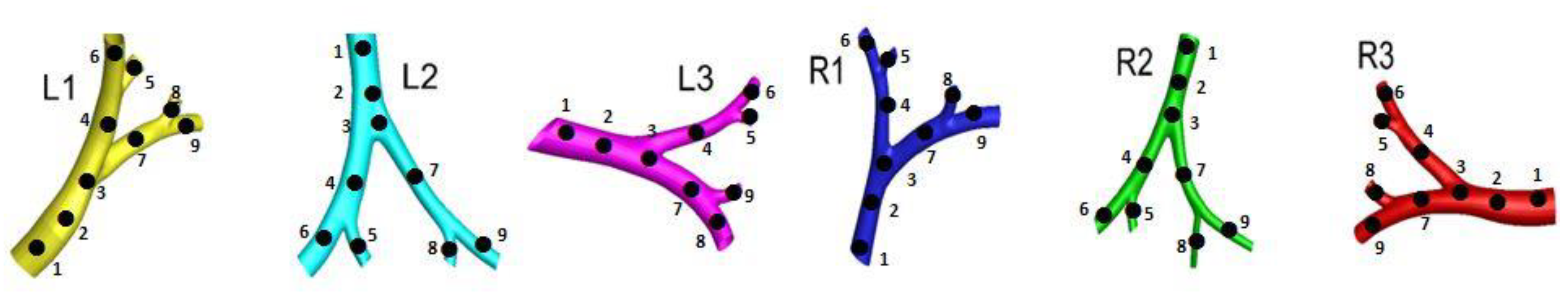
Mechanical Ventilation(Inhalation, t = 0.3 s)Pressure Ratio, Pn(α)Shear Stress Ratio, S(β)
P1P2P3P4P5P6P7P8P9S1S2S3S4S5S6S7S8S9
Whole lung vs. L10.961.061.0311.030.9211.091.041.031.020.881.050.940.961.020.951.02
Whole lung vs. L21.050.981.0710.990.930.970.971.021.020.980.970.960.991.021.041.011.02
Whole lung vs. L31.011.021.041.011.111.030.991.021.021.021.060.941.011.011.051.031.051.01
Normal Breathing (inhalation, t = 0.9 s)Pressure ratio, P(α)Shear stress ratio, S(β)
P1P2P3P4P5P6P7P8P9S1S2S3S4S5S6S7S8S9
Whole lung vs. R11.010.971.021.110.991.080.990.991.010.971.021.051.011.0310.981.021.02
Whole lung vs. R21.011.010.9911.041.010.991.011.021.0410.980.990.931.010.990.980.95
Whole lung vs. R30.9910.980.990.880.9810.981.021.130.960.990.971.031.041.041.051.08
Publisher’s Note: MDPI stays neutral with regard to jurisdictional claims in published maps and institutional affiliations.

