Article

Geometry and Flow Properties Affect the Phase Shift between Pressure and Shear Stress Waves in Blood Vessels

1
Interdisciplinary Center for Advanced Materials Simulation (ICAMS), Ruhr-Universität Bochum, 44801 Bochum, Germany
2
School of Engineering, Institute for Multiscale Thermofluids, University of Edinburgh, Edinburgh EH9 3FB, UK
*
Authors to whom correspondence should be addressed.
Fluids 2021, 6(11), 378; https://doi.org/10.3390/fluids6110378
Submission received: 24 August 2021 / Revised: 13 October 2021 / Accepted: 20 October 2021 / Published: 23 October 2021
(This article belongs to the Special Issue Computational Biofluiddynamics: Advances and Applications)

Abstract

:
The phase shift between pressure and wall shear stress (WSS) has been associated with vascular diseases such as atherosclerosis and aneurysms. The present study aims to understand the effects of geometry and flow properties on the phase shift under the stiff wall assumption, using an immersed-boundary-lattice-Boltzmann method. For pulsatile flow in a straight pipe, the phase shift is known to increase with the Womersley number, but is independent of the flow speed (or the Reynolds number). For a complex geometry, such as a curved pipe, however, we find that the phase shift develops a strong dependence on the geometry and Reynolds number. We observed that the phase shift at the inner bend of the curved vessel and in the aneurysm dome is larger than that in a straight pipe. Moreover, the geometry affects the connection between the phase shift and other WSS-related metrics, such as time-averaged WSS (TAWSS). For straight and curved blood vessels, the phase shift behaves qualitatively similarly to and can thus be represented by the TAWSS, which is a widely used hemodynamic index. However, these observables significantly differ in other geometries, such as in aneurysms. In such cases, one needs to consider the phase shift as an independent quantity that may carry additional valuable information compared to well-established metrics.

1. Introduction

Cardiovascular diseases such as atherosclerosis and aneurysms are the leading cause of mortality globally [1]. Atherosclerotic plaques, which generally make vascular walls vulnerable, can form on aneurysms [2,3,4,5].
Hemodynamic forces, such as pressure and wall shear stress (WSS), play an important role in vascular physiology and pathology [6,7,8]. The interaction between tensile and shear stresses has been widely reported to play a crucial role in endothelial behavior [9,10]. The flow-induced WSS is time varying due to the pulsatile nature of blood flow. The phase shift (temporal delay) between the pressure and WSS on the endothelium is a primary parameter that characterizes the interaction between these two forces [11] and is closely associated with vascular diseases [12,13].
It has been suggested that the phase shift is important in vascular regulation and remodeling [14] and in predicting sites prone to atherosclerosis in the coronary artery [11], the carotid artery [15], and arterial stenosis [16]. It has been proposed by several independent researchers that a large phase shift occurs in regions where atherosclerotic lesions are prevalent [16,17,18,19,20]. Moreover, Maul et al. [21] reported that the magnitude and/or frequency of these mechanical stimuli affect the morphology, growth, and differentiation of mesenchymal stem cells in the vasculature. Owatverot et al. [22] performed an analysis of concurrent tensile and shear stresses and highlighted their influence on the behaviors of endothelial and stem cells. The phase shift has also been shown to significantly affect the strain energy density of the endothelial cell where mechanotransduction is prevalent [23]. Shojaei et al. [24] reported that the phase shift regulates the differentiation of human-adipose-derived stem cells toward the endothelial phenotype.
It has been further noted that the phase shift influences proatherogenic responses in endothelial cells and is an important parameter characterizing arterial susceptibility to disease [25,26]. These observations are consistent with the understanding at the cellular or molecular level: the endothelial monolayer senses the phasic change between pulsating pressure and WSS and alters its cellular actions, in particular nitric oxide production [19,27]. Atherosclerotic plaques have been reported to be also closely associated with a low time-averaged WSS (TAWSS) [28,29,30] and a high temporal WSS gradient (TWSSG) [31,32,33].
As to the underlying physical mechanism for the phase shift, it is noteworthy that pressure fluctuations propagate with the speed of sound. This process is fast compared to variations of the fluid velocity field and of its spatial gradients, the latter determining the stress tensor. As a consequence, one expects a time delay and thus a phase shift between pressure and shear stress signals. While this issue can be addressed by analytic means for a pulsatile flow in a straight tube (see the Womersley solution below), numerical modeling is necessary to address this issue in more complex geometries.
Indeed, little is known about the effects of complex vessel geometry and fluid flow properties on the phase shift and on the possible correlation among the WSS-based quantities, such as the phase shift, the TAWSS, and the TWSSG. There is probably a coupled causality: geometry alters flow (short-term effect), and flow changes geometry (long-term effect). In the present study, we aim to investigate the first case and assess the hypothesis that geometry alone can play a crucial role in the phase shift. In principle, the pulsatile deformation of an artery (or aneurysm) may also have some effects on the time delay. As a first step, however, the focus of this work is to understand the roles the geometric and flow parameters play under the rigid (or stiff) [34,35] wall assumption.
In this work, we employed lattice-Boltzmann simulations of flow in differently shaped blood vessels (Figure 1) to study the change of the phase shift with geometry, the Womersley number (flow pulsatility), and the Reynolds number (flow speed). We found that geometry has a strong effect on the phase shift. While the phase shift is closely correlated with other observables, such as the TAWSS, in straight or slightly curved blood vessels, it was observed to become unpredictable within an aneurysm, which might accelerate the development of vulnerable regions and eventually the rupture of the blood vessel.
The paper is organized as follows. Relevant physical aspects are introduced in Section 2. The numerical methods and benchmark tests are presented in Section 3 and Section 4. The simulation results of sinusoidal flow in differently shaped domains are presented and discussed in Section 5, with a particular focus on the geometrical effect. Section 6 provides a summary of the work with an outlook for future studies.

2. Physical Model

Throughout this study, it was assumed that the fluid (blood) can be represented as an incompressible fluid with uniform density. The continuum assumption is justified by the large diameter of the blood vessel considered in this study (a few millimeters up to centimeters) as compared to the typical size of the particulate objects (red blood cells, platelets, and white blood cells, which typically lie in the range 2–20 μm). Thus, the particulate properties [36,37] of the blood were not considered here. We thus sought to solve the underlying Navier–Stokes equations in the incompressible limit. It is noteworthy that the methodology implemented here—the lattice Boltzmann method (LBM)—allows for a small, but finite numerical compressibility. It turns out that this feature is not necessarily a drawback. Rather, if used adequately—e.g., by introducing multiple relaxation times (MRTs) within LBM; see Section 3—it may lead to better stability of the numerical scheme.

2.1. Physical Ingredients

In principle, the circumferential stretch of a blood vessel is dominated by the so-called transmural pressure, which represents the pressure difference on both sides of the vessel wall. The external (or intracranial) pressure is normally one order of magnitude smaller than the intra-artery pressure and is often neglected in most existing models [38,39,40,41]. Hence, the temporal variation of the transmural pressure (or circumferential stretch) mainly depends on the pressure inside the artery or aneurysm.
The pressure pulse generated by the heart is a composite wave consisting of multiple harmonic components. Each harmonic component is a sine or cosine wave with different amplitude and frequency. In this work, we used a single sine curve to represent the input signals in order to focus on fundamental physical aspects.
Without loss of generality, this work: (1) used a toy model and focused on a short segment (patch) of the blood circulatory system; (2) assumed that the waveform of pressure at the inlet and outlet is known and sinusoidal; any change in the inlet/outlet pressure was treated as an input to the simulation; (3) focused on WSS since the pressure signal has a long wavelength and its traveling time is negligibly short (see Appendix A for more details).
The phase shift between the pressure, P, and WSS, σ w , is characterized by the phase shift, Δ φ , in degrees (as adopted in [42,43]):
Δ φ = t ( σ w max ) t ( P max ) T × 360
where t ( P max ) and t ( σ w max ) , respectively, indicate the peak pressure and WSS times within one cardiac cycle of duration T (Figure 2). The phase shift is positive when the pressure signal reaches its maximum before the WSS signal and negative if the pressure lags behind the WSS.
As discussed in Appendix A, it is reasonable to assume that the maximum pressure time at any point of the short vessel considered in this work is equal to the peak time of the input pressure signal, i.e., t ( P max ) = T / 4 for the entire vessel since the pressure signal in our model is a sine wave.
Besides the phase shift, the temporal distribution of WSS is also quantified by the time-averaged wall shear stress (TAWSS) and the temporal WSS gradient (TWSSG). The TAWSS is determined by integrating the WSS magnitude at each point x over one period [44]:
TAWSS ( x ) = 1 T 0 T σ w ( x , t ) d t .
The TWSSG quantifies the average rate of change in WSS over half a cardiac cycle [32,33],
TWSSG ( x ) = σ w max ( x ) σ w min ( x ) T / 2 ,
where σ w max ( x ) and σ w min ( x ) indicate the maximum and minimum values of WSS at x and within the considered time interval.

2.2. Dimensionless Groups

The dimensionless numbers that are relevant to this work can be defined as ratios of the physical time scales mentioned in Appendix A: the Reynolds number, which describes the ratio of inertial to viscous interactions, Re = U D / ν = ( 2 L / R ) t ν / t u , where R and L, respectively, indicate the radius and length of the vessel ( L / R = 12 and diameter D = 2 R ), ν is the kinematic viscosity, U indicates the mean flow velocity, and t ν and t u indicate the momentum diffusion and advection times, respectively; the Womersley number, which characterizes the pulsatile flow frequency in relation to viscous effects, α = R ω / ν = 2 π t ν / T , where ω is the angular frequency ( ω = 2 π / T with T indicating the period). The last ratio is the Mach number, Ma t s / t u , with t s representing the sound wave (or acoustic) time, which is not of interest in the context of this work as it is always small in blood flow.

3. Numerical Model

In this work, the standard incompressible Navier–Stokes equations of fluid dynamics in three dimensions were solved using a standard lattice Boltzmann method on a D3Q19 lattice with the multiple-relaxation-time collision operator [45]. The coupling between the fluid and vessel wall was realized via the immersed boundary method [46]. The use of the MRT scheme within LBM allows tuning the relaxation parameters such that both the accuracy and stability of the numerical scheme are improved [45]. This feature is particularly important at high Reynolds numbers, where small fluctuations may quickly grow due to enhanced nonlinearity. The method and the underlying in-house software were tested versus semi-analytic results by Krüger et al [47]. Further applications of the software include suspensions of deformable red blood cells [36,48,49] and compliant blood vessels [50].
The effect of the mesh size on the numerical accuracy of the present model was already addressed in [47]. Based on the experience gained from this work and a more recent study [50], we found that, within given constraints on the computation time, a mean effective spatial resolution (mesh size) of approximately 0.087 mm provides very good results. As will be shown below (see Section 4), with this choice, the simulations reproduced the predicted phase shift within an error of less than 2%. The fluid domain consisted of approximately 3.7 million lattice nodes. The blood vessel (immersed structure) consisted of approximately 82,000 nodes. The discrete time step was set to d t = 6.7 × 10 6 s; for a cycle with a duration of 0.8 s, the temporal resolution was approximately 120,000 time steps per cycle. Typically, each cycle ran for approximately 40 h in serial on a workstation with Intel® Xeon(R) CPU E5-1620 v2 @ 3.70GHz.
The limit of a quasi-rigid tube wall was achieved by assigning stiff springs on the entire wall, together with making all elastic moduli as large as possible; this is the same treatment as in [50].
In lattice-Boltzmann simulations, the numerical speed of sound is generally smaller than that in reality; it was 7.6 m/s in our simulations. Nevertheless, all physical time scales (Appendix A) that were resolved were sufficiently long compared to the numerical sound propagation time. Using the parameters of the present study, it is easy to verify that t ν = 356 t s , t ω = 270 t s , t u = 44 t s , and t ρ u = 45 t s , where t ω and t ρ u indicate the oscillation and inertial times, respectively. Neglecting sound propagation is thus a good approximation in the present study. Throughout this work, the peak WSS time, t ( σ w max ) , was extracted by curve fitting to a sinusoidal function, using simulated data within a short time interval of T / 4 around each peak time. As justified in Appendix A, we set for the entire tube t ( P max ) = T / 4 .
We used the pressure-corrected periodic boundary conditions [51] to prescribe an intended pressure drop between the two ends of the blood vessel to drive flow, together with applying periodicity to fluid velocity. The no-slip condition at the wall was recovered by the employed immersed boundary method.

4. Validation

The accuracy of the present model in the quantitative analysis of the phase shift (or peak shear stress time, t ( σ w max ) ) is demonstrated as follows. For flow through a straight pipe, driven by a sinusoidal pressure gradient:
P ( t ) = P 0 [ 1 + sin ( ω t ) ] = P 0 [ 1 + sin ( 2 π t / T ) ] ,
the phase shift Δ φ between waves of WSS and pressure can be expressed as a function of the Womersley number α [52],
Δ φ ( α ) = arctan D ( α ) C ( α ) ,
where:
C ( α ) = ber ( α ) bei ( α ) bei ( α ) ber ( α ) ber 2 ( α ) bei 2 ( α ) , D ( α ) = ber ( α ) ber ( α ) bei ( α ) bei ( α ) ber 2 ( α ) bei 2 ( α )
with ber ( · ) and bei ( · ) representing the derivatives of Kelvin functions ber ( · ) and bei ( · ) , respectively.
Simulation parameters relevant for this validation are given in Table 1. We used a Python script to calculate the analytical phase shift by evaluating Equation (5). Throughout this work, we used Equation (1) to determine the phase shift from the simulations. As illustrated in Figure 3, the maximum relative error of our simulation results from the corresponding analytical solutions was less than 2% when averaging over the entire tube wall. Without such averaging, the maximum local error was 5.7%.

5. Results and Discussion
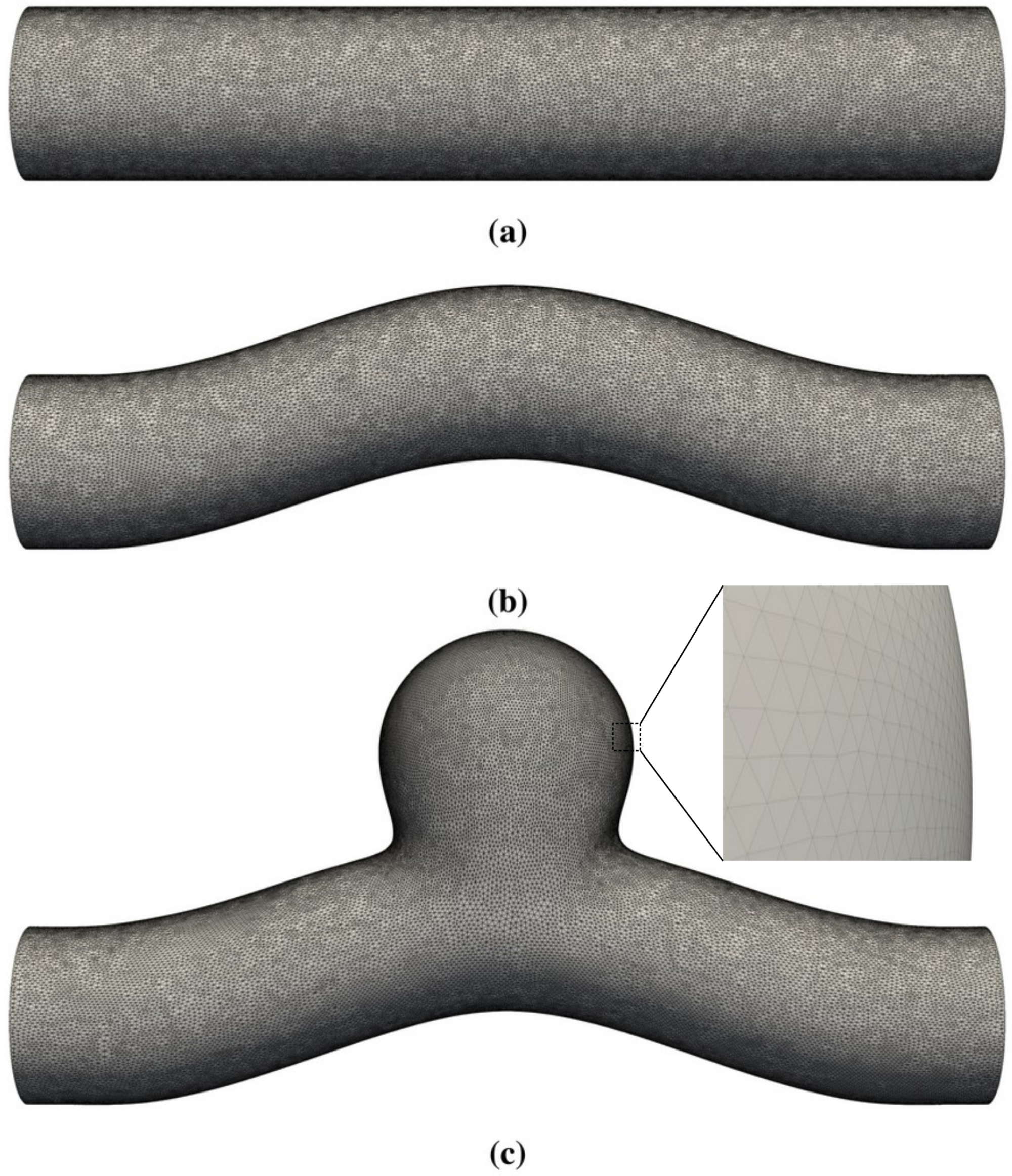
Unless otherwise stated, the simulation parameters given in Table 2 were used; the sinusoidal pressure gradient shown in Equation (4) was used for all simulations. The corresponding Reynolds and Womersley numbers were Re = 179 and α = 2.88 , respectively, which are typical for cerebral blood flow. Based on sinusoidal flow in a straight cylindrical tube, we can define three characteristic quantities: spatiotemporal average of flow velocity, U = P ¯ R 2 / 8 η = 0.17 m/s; time-averaged wall shear stress, TAWSS = 3 P 0 R / 4 = 2 Pa; temporal WSS gradient, TWSSG = P 0 R / T = 3.4 Pa/s.

5.1. Study Cases

To disentangle the effects of wall geometry and fluid flow on the phase shift between pressure and WSS, we considered two different sets of simulations:
  • First, we focused on the effect of flow. We performed the simulations of sinusoidal flow through a curved tube without an aneurysm (Figure 1b). We varied the flow properties in two ways:
    (a)
    Varying the Womersley number α while keeping the Reynolds number Re fixed. This was achieved by changing the period T: α = 1.56 , 2.0, and 2.88 for T = 2.72 s, 1.6 s, and 0.8 s, respectively (see Figure 4). Note that the average flow speed (and thus Re) depends on α . Therefore, one also needs to change the pressure drop to maintain a given value of Re;
    (b)
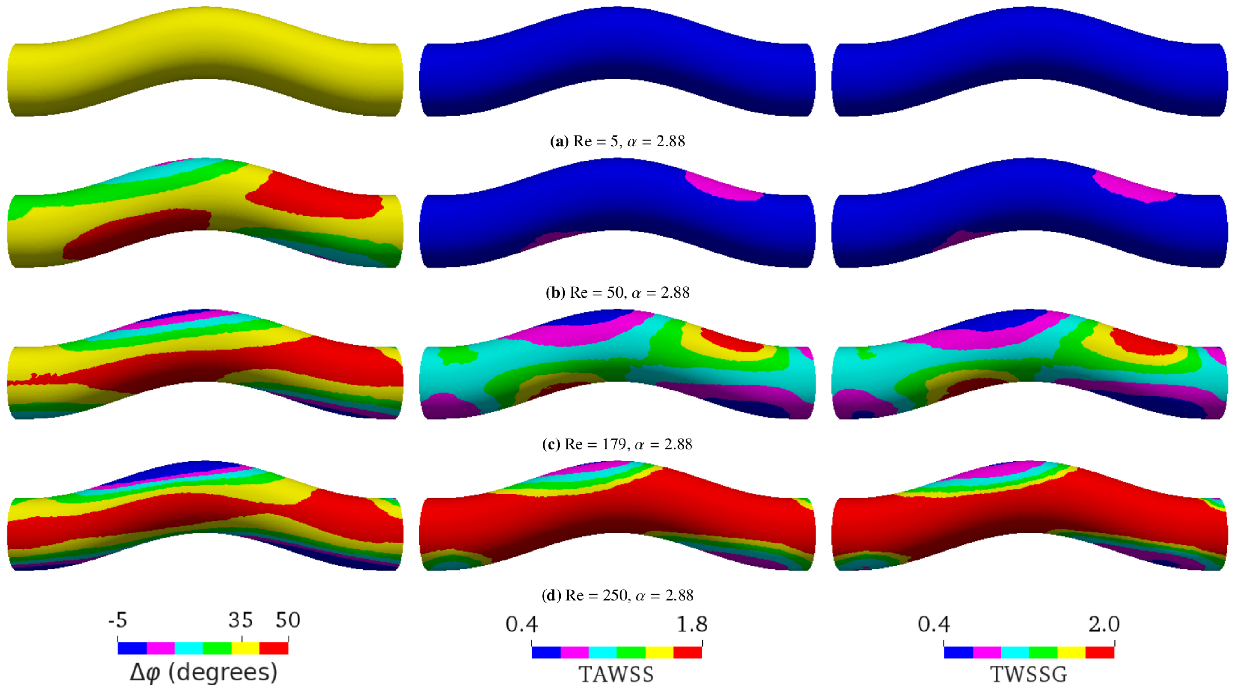
    Varying only Re by altering the flow speed via the amplitude of the pressure gradient: Re = 5, 50, 179, or 250 as a result of changing the average flow velocity to 0.00475 m/s, 0.0475 m/s, 0.17 m/s, or 0.2375 m/s, respectively (see Figure 5);
  • In the second set of simulations, we used three different geometries (Figure 1) and kept the flow properties identical: the average flow velocity, Reynolds, and Womersley numbers were 0.17 m/s, 179, and 2.88, respectively (see Figure 6).
Each simulation was performed for a total duration of three cardiac cycles, which is sufficient to reach a time-periodic flow field.

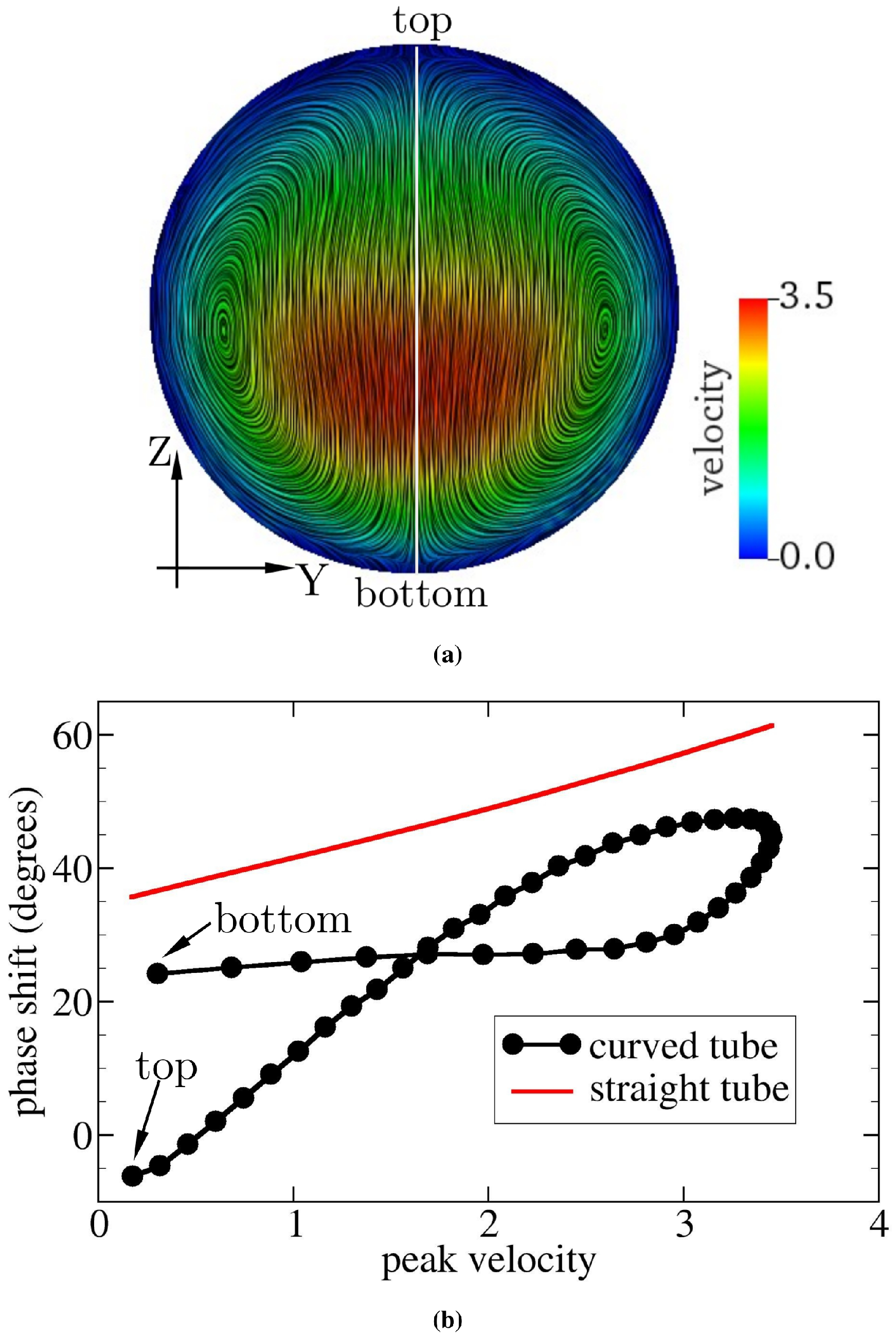
5.2. Varying Flow Properties in a Curved Tube without Aneurysm

The phase shift between the pressure and WSS waves, Δ φ , is affected by several factors. We started with the role of fluid flow properties, in particular the Womersley and Reynolds numbers, α and Re.
In a straight tube, Δ φ is the same on every point of the tube surface, and it increases with α , ranging from 0 to 45 (Figure 3). We observed that, in a curved tube, Δ φ becomes inhomogeneous (Figure 4). While the average value of Δ φ increases with α , the variation of Δ φ also increases with α , and Δ φ can reach local values larger than 45 for sufficiently high α . In agreement with the calculations in [53], we observed that the TAWSS and TWSSG increase with α . Additionally, our simulations showed that both TAWSS and TWSSG become increasingly heterogeneous with α . A key feature emerging with increasing α is the formation of regions opposite each other where Δ φ , the TAWSS, and the TWSSG assume low and large values, respectively. Following the flow entering the tube from the left in Figure 4, the flow is first forced upward at the bend, resulting in an increase of Δ φ , the TAWSS, and the TWSSG at the bottom of the tube and a decrease at the top. In the second half of the bend, when the flow is forced downward again, the trend reverses, and the observables assume larger value at the top of the tube and lower values at the bottom.
As shown by Equation (5), Δ φ in a straight tube is a function of α only. In particular, Δ φ does not depend on Reynolds numbers. Our simulations confirmed the independence of Δ φ on Re when the tube is not curved (data not shown). For a curved pipe, however, we found that Re also largely controls Δ φ ; a higher Re leads to a larger Δ φ (Figure 5). The spatial distribution of Δ φ is homogeneous at the lowest Re investigated (Figure 5a). It then becomes increasingly heterogeneous as Re is raised from 5 to 179 (Figure 5b,c). This spatial heterogeneity seems to saturate and even decrease upon the further increase of Re (Figure 5d). Surprisingly, Δ φ can even reach negative values in certain places for sufficiently large Re. Similar to Figure 4, increasing Re also leads to the formation of two pairs of oppositely located patches with locally small and large values of Δ φ , the TAWSS, and the TWSSG.
It is noteworthy that the variations of the simulation parameters have no impact on Δ φ , as long as Re and α are kept constant. For example, compared with the case shown in Figure 4a, a simulation with 3.4-times higher flow speed, viscosity, and frequency (but fixed α = 1.56 and Re = 50) gave the same distribution and values of Δ φ (data not shown). This result simply confirms the law of similarity, which states that dimensional parameters, such as the flow rate and period, influence the flow field (except for its absolute magnitude), only through dimensionless numbers, such as Re and α .

5.3. Curved Tube with Aneurysm

We saw that, besides the flow properties, the geometry also affects the phase shift Δ φ between the pressure and shear stress signals. In the case of pulsatile flow in a straight tube, Δ φ is the same everywhere in the tube (Figure 6a) if we neglect small numerical errors due to discretization of the geometry. However, we found that Δ φ varies in space for other geometries, such as the curved tube (Figure 6b) and the curved tube with aneurysm (Figure 6c).
Figure 4 and Figure 5 show that the effect of geometry on Δ φ , the TAWSS, and the TWSSG is enhanced when the Womersley number α and/or Reynolds number Re increase. Compared to the straight vessel, the phase shift increases at the inner bend of the curved vessel and inside the aneurysm dome. The strongest effect of geometry on Δ φ was observed in a curved tube containing an aneurysm, where the spatial behavior of Δ φ becomes highly irregular (Figure 6c). This behavior must be caused by the complex flow field, including nontrivial backflow effects, that prevails in the aneurysmal dome.
Importantly, the geometry considerably affects the connection between Δ φ and other WSS-based metrics, such as the TAWSS and the TWSSG (Figure 6 and Figure 7). Given that the imposed signal is a sine wave, it was expected that the TAWSS and TWSSG would provide qualitatively the same type of information (see the similarity of the distribution of the TAWSS and TWSSG in Figure 6).
Besides the strong similarity between the TAWSS and TWSSG in all investigated geometries, we found that Δ φ and the TAWSS in the curved tube are closely correlated as well: Δ φ is large in places where the TAWSS is high and small or even negative where the TAWSS is low (Figure 7a,b).
The correlation between Δ φ and the TAWSS seems to be lost as the flow inside the aneurysm dome becomes less regular. A possible rationale for this observation could be that velocity fluctuations are enhanced due to the nonlinearity of the fluid dynamics equations in the investigated inertial flow regime. This interpretation is in line with the observation that the phase shift grows as the Reynolds number increases (see Figure 5). Velocity fluctuations may be of a purely numerical nature, but may also arise from the irregularities of the geometric structure. Since the correlation between the shear stress and phase shift persists in the case of the curved tube without aneurysm, we concluded that fluctuations arising from geometry (possibly augmented by grid resolution effects) are the dominant reason for the loss of correlations in the aneurysm dome (Figure 7c).
It seems that Δ φ and the TAWSS can be used as proxy metrics for each other, as long as the geometry and flow field are sufficiently smooth. Contrarily, the flow field in an aneurysmal dome is complex, and the TAWSS and Δ φ show different behaviors. In principle, the combined effects of a low TAWSS and a large variation of Δ φ in the aneurysm may trigger biological processes that could impair the mechanical stability of the endothelium over a long period of time. A more careful examination of the sensitivity of these biological processes seems justified.
Flow is sensitive to geometry, which can, in turn, induce significant differences in the phase shift, Δ φ . If Δ φ were determined solely by the primary (axial) flow, Δ φ would be essentially the same everywhere. Due to the observed dependence of Δ φ on Re and tube curvature, it seems that the spatial variation of Δ φ is closely related to secondary flows [54] that appear in complex geometries when inertia is not negligible. Due to inertia, a perturbation in pressure takes some finite time to be visible in the surrounding velocity field, and consequently in WSS. Thus, for simple geometries such as a straight tube, WSS lags behind the pressure and Δ φ > 0 (Figure 3 and Figure 6a). Yet, Δ φ < 0 can occur due to geometrical effects. While laminar flow in a straight tube is perfectly axial, in a curved tube (Figure 6b), the curvature leads to secondary flows within the plane perpendicular to the axial direction. This is illustrated in Figure 8a, which shows the cross-section of the curved tube midway between the inlet and outlet. We observed that the magnitude and features of the secondary flows depend on the tube curvature and the flow properties, in particular Re, which affect the mechanism of momentum transport (data not shown). For flow in a straight tube, WSS is determined purely by the radial diffusion of momentum due to viscosity. When the geometry is curved, however, WSS can also be influenced by the diffusion and advection of momentum via secondary flows.
The curvature of the tube induces centripetal forces in the fluid, which move the line of maximum velocity away from the centerline of the tube towards either the bottom or the top of the tube. From Figure 8a, it can be seen that the flow is shifted towards the bottom of the cross-section, leaving the top wall with a lower velocity and WSS (see the TAWSS in Figure 6b). Figure 8b tells us that, in the presence of curvature, the delay between pressure and velocity signals is the largest for the region within the channel with the maximum velocity (the rightmost data in Figure 8b). Moreover, the variation of Δ φ when approaching the vessel wall is nonsymmetric, as it seems to saturate on a plateau towards the bottom wall, but decreases approximately linearly when moving towards the upper vessel boundary. There exist three possible sources of velocity (or WSS) variation: radial diffusion of momentum, radial advection of momentum, and centrifugal acceleration (or force). The last term drives the secondary flow and acts as an additional pressure gradient. We speculated that the phase shift between the pressure and WSS signals is controlled by the combined effects of these three sources. Although the detailed mechanisms underlying the phase shift remain unclear, we can conclude that the axial advective transport of momentum no longer dominates the phase shift, provided that the pipe (or vessel) is not straight.
We found that the observed phase shift is a complicated function of velocity field, geometry, and flow parameters (Re and α ). There do not seem to exist simple scaling laws for Δ φ that could be used to predict the local phase shift in a given geometry without running a full simulation of the flow field. At the current stage, a predictive model for Δ φ is not yet available, and the present work thus emphasizes the need for further research.

6. Conclusions

The phase shift (or time delay) between pressure and wall shear stress (WSS) signals can elicit pathological responses in endothelial cells and play a crucial role in diseases, such as atherosclerosis and brain aneurysms. In this work, we employed a hybrid immersed-boundary-lattice-Boltzmann method to investigate the phase shift, with the focus on the effects of flow oscillation and inertia (via Womersley and Reynolds numbers) and wall geometry (straight tube, curved tube, and curved tube with an aneurysm). The accuracy of the method was shown through pulsatile Womersley flow tests using a straight rigid pipe.
For pulsatile flow in a straight tube, the phase shift between the pressure and WSS increases with the Womersley number, but is independent of the Reynolds number (or flow speed). Within a curved tube, the phase shift shows a strong dependence on the Reynolds number as well, an effect that is caused by inertial momentum transport from the tube centerline to the walls. Importantly, we found highly heterogeneous distributions of the phase shift within the aneurysmal dome.
While there is no simple way to precisely predict how the phase shift behaves in an even slightly complex geometry, we found that the phase shift is well correlated with the time-averaged wall shear stress (TAWSS) and the temporal wall shear stress gradient (TWSSG) in the curved tube, outside of the aneurysm. Interestingly, the strong correlation between the phase shift and the TAWSS/TWSSG is lost within the aneurysmal dome. Our findings, therefore, suggest that the phase shift could be used as an independent flow metric in segments of complex geometry where the influence of the flow on the blood vessel wall is not reliably characterized by WSS alone. We speculate that geometries with an uncorrelated phase shift and WSS patterns might be particularly relevant to long-term detrimental biological effects that weaken the blood vessel integrity eventually.
A quantitative predictive model for the phase shift as a function of geometry and flow parameters (Reynolds and Womersley numbers) is not yet available. The phase shift seems to depend strongly on the details of the secondary flows that arise in curved geometries at finite inertia. At the current stage, a full flow simulation is necessary to predict the phase shift distribution in a given geometry. More research into the underlying physical mechanisms of the phase shift seems warranted.
In this work, blood vessel walls were assumed to be rigid and the effect of red blood cells were neglected. We expect that the flexibility of the vessel wall and the particulate properties of blood may also play a role in the phase shift between pressure and shear stress signals. A thorough study of this issue provides a challenging task for future work.

Author Contributions

Conceptualization, H.W., T.K., and F.V.; data curation, H.W.; formal analysis, H.W.; funding acquisition, T.K. and F.V.; investigation, H.W.; methodology, H.W., T.K., and F.V.; project administration, F.V.; resources, H.W.; software, H.W. and T.K.; supervision, T.K. and F.V.; validation, H.W.; visualization, H.W.; writing—original draft, H.W.; writing—review and editing, H.W., T.K., and F.V. All authors have read and agreed to the published version of the manuscript.

Funding

T.K. received funding from the European Research Council (ERC) under the European Union’s Horizon 2020 Research and Innovation Programme (Grant Agreement No. 803553).

Acknowledgments

H.W. acknowledges his IMPRS-SurMat scholarship and the financial support by the STKS department at ICAMS, the Ruhr-Universität Bochum. ICAMS acknowledges funding from its industrial sponsors, the state of North-Rhine Westphalia, and the European Commission in the framework of the European Regional Development Fund (ERDF). We acknowledge support by the DFG Open Access Publication Funds of the Ruhr-Universität Bochum.

Conflicts of Interest

The authors declare no conflict of interest. The funders had no role in the design of the study; in the collection, analyses, or interpretation of the data; in the writing of the manuscript; nor in the decision to publish the results.

Appendix A. Time Scales

The pressure signal propagates at the speed of sound. The shear stress has two transport mechanisms: advection and momentum diffusion. For flow in a straight tube, advection is only along the flow direction and therefore does not contribute to the radial transport near the wall where the flow is tangential and slow compared to the tube center. Therefore, in a straight tube, WSS is determined by momentum diffusion. For flow in a curved vessel, however, there can be significant advection from the centerline to an area close to the wall due to inertia and geometry-induced secondary flow. In that case, the overall transport of shear stress from the centerline to the vessel surface will not just be due to diffusion.
Upon a first view, the phase shift might be associated with five physical time scales: momentum diffusion time t ν R 2 / ν , inertial time t ρ u ρ U / P 0 , oscillation time t ω 2 π / ω = T , sound wave (or acoustic) time t s = L / c s , and advection time t u L / U t s / Ma . Here, R and L, respectively, indicate the radius and length of the tube or blood vessel; ν is the kinematic viscosity, ν = η / ρ , where η and ρ , respectively, represent the dynamic viscosity and the fluid density; U indicates the mean flow velocity; P 0 is the amplitude of pulsatile pressure gradient; ω is the angular frequency ( ω = 2 π / T with T indicating the period); c s is the speed of sound; Ma denotes the Mach number.
For pulsatile flow in a straight rigid pipe, the total mean (i.e., spatiotemporal average) velocity U is U = P ¯ R 2 / ( 8 η ) where P ¯ indicates the time average of the pressure gradient [52], e.g., P ¯ = 1 T 0 T P ( t ) d t = 1 T 0 T P 0 ( A sin ( ω t ) + B ) d t = B P 0 where A and B are constants. Thus, the inertial time can be written as t ρ u ρ U / P 0 = P ¯ R 2 / ( 8 ν P 0 ) = B R 2 / ( 8 ν ) = t ν B / 8 , i.e., t ρ u t ν . Hence, in the present problem, there are only four independent times: the momentum diffusion time t ν , the oscillation time t ω , the advection time t u , and the acoustic time t s .
The speed of sound, c s , in blood is roughly 1570 m/s. The radius, R, of major cerebral arteries is about 2 mm. In experiments or simulations, a length-to-diameter ratio no less than five is generally a good choice. In this work, we used L / R = 12 . Blood density ρ and dynamic viscosity η are normally within the range of 1–1.06 g/cm 3 and 3–4 mPa s, respectively. The period of the human heartbeat (or the period of pulsatile pressure), T, is 0.8 s in normal cases. Given the above parameters, the traveling time of the pressure signal along the short pipe considered in this work was only 2 · 10 5 T , which is negligible compared to all other physically relevant times.

References

  1. World Health Organization, Regional Office for Europe. Global atlas on Cardiovascular Disease Prevention and Control: Published by the World Health Organization in Collaboration with the World Heart Federation and the World Stroke Organization; World Health Organization, Regional Office for Europe: Copenhagen, Denmark, 2011; 155p. [Google Scholar]
  2. Tateshima, S.; Tanishita, K.; Omura, H.; Sayre, J.; Villablanca, J.; Martin, N.; Vinuela, F. Intra-aneurysmal hemodynamics in a large middle cerebral artery aneurysm with wall atherosclerosis. Surg. Neurol. 2008, 70, 454–462. [Google Scholar] [CrossRef]
  3. Yang, J.; Cui, C.; Wu, C. Cerebrovascular hemodynamics in patients with cerebral arteriosclerosis. Neural Regen. Res. 2011, 6, 2532–2536. [Google Scholar]
  4. Sugiyama, S.; Niizuma, K.; Nakayama, T.; Shimizu, H.; Endo, H.; Inoue, T.; Fujimura, M.; Ohta, M.; Takahashi, A.; Tominaga, T. Relative residence time prolongation in intracranial aneurysms: A possible association with atherosclerosis. Neurosurgery 2013, 73, 767–776. [Google Scholar] [CrossRef]
  5. Bae, H.; Choi, J.; Kim, B.; Lee, K.; Shin, Y. Predictors of Atherosclerotic Change in Unruptured Intracranial Aneurysms and Parent Arteries During Clipping. World Neurosurg. 2019, 130, e338–e343. [Google Scholar] [CrossRef] [PubMed]
  6. Cunningham, K.; Gotlieb, A. The role of shear stress in the pathogenesis of atherosclerosis. Lab. Investig. 2005, 85, 9–23. [Google Scholar] [CrossRef] [PubMed] [Green Version]
  7. Chiu, J.J.; Usami, S.; Chien, S. Vascular endothelial responses to altered shear stress: Pathologic implications for atherosclerosis. Ann. Med. 2009, 41, 19–28. [Google Scholar] [CrossRef]
  8. Evans, P.; Kwak, B. Biomechanical factors in cardiovascular disease. Cardiovasc. Res. 2013, 99, 229–231. [Google Scholar] [CrossRef] [Green Version]
  9. Steinman, D.; Thomas, J.; Ladak, H.; Milner, J.; Rutt, B.; Spence, J. Reconstruction of carotid bifurcation hemodynamics and wall thickness using computational fluid dynamics and MRI. Magn. Reson. Med. 2002, 47, 149–159. [Google Scholar] [CrossRef]
  10. Joshi, A.; Leask, R.; Myers, J.; Ojha, M.; Butany, J.; Ethier, C. Intimal thickness is not associated with wall shear stress patterns in the human right coronary artery. Arterioscler. Thromb. Vasc. Biol. 2004, 24, 2408–2413. [Google Scholar] [CrossRef] [Green Version]
  11. Torii, R.; Wood, N.; Hadjiloizou, N.; Dowsey, A.; Wright, A.; Hughes, A.; Davies, J.; Francis, D.; Mayet, J.; Yang, G.; et al. Stress phase angle depicts differences in coronary artery hemodynamics due to changes in flow and geometry after percutaneous coronary intervention. Am. J. Physiol. Heart Circ. Physiol. 2009, 296, H765–H776. [Google Scholar] [CrossRef] [Green Version]
  12. Tarbell, J.; Shi, Z.; Dunn, J.; Jo, H. Fluid Mechanics, Arterial Disease, and Gene Expression. Annu. Rev. Fluid Mech. 2014, 46, 591–614. [Google Scholar] [CrossRef] [Green Version]
  13. Al-Rawi, M.; Al-Jumaily, A.; Lowe, A. Stress Phase Angle for Non-Invasive Diagnosis of Cardiovascular Diseases. In Proceedings of the ASME International Mechanical Engineering Congress and Exposition, Proceedings (IMECE), Vancouver, BC, Canada, 12–18 November 2010; Volume 2, pp. 747–749. [Google Scholar] [CrossRef]
  14. Qiu, Y.; Tarbell, J. Interaction between wall shear stress and circumferential strain affects endothelial cell biochemical production. J. Vasc. Res. 2000, 37, 147–157. [Google Scholar] [CrossRef] [PubMed]
  15. Makris, G.; Nicolaides, A.; Xu, X.; Geroulakos, G. Introduction to the biomechanics of carotid plaque pathogenesis and rupture: Review of the clinical evidence. Br. J. Radiol. 2010, 83, 729–735. [Google Scholar] [CrossRef] [Green Version]
  16. Sadeghi, M.; Shirani, E.; Tafazzoli-Shadpour, M.; Samaee, M. The effects of stenosis severity on the hemodynamic parameters-assessment of the correlation between stress phase angle and wall shear stress. J. Biomech. 2011, 44, 2614–2626. [Google Scholar] [CrossRef]
  17. Qiu, Y.; Tarbell, J. Numerical simulation of pulsatile flow in a compliant curved tube model of a coronary artery. J. Biomech. Eng. 2000, 122, 77–85. [Google Scholar] [CrossRef]
  18. Tada, S.; Tarbell, J. A Computational Study of Flow in a Compliant Carotid Bifurcation-Stress Phase Angle Correlation with Shear Stress. Ann. Biomed. Eng. 2005, 33, 1202–1212. [Google Scholar] [CrossRef] [PubMed]
  19. Dancu, M.; Tarbell, J. Large Negative Stress Phase Angle (SPA) attenuates nitric oxide production in bovine aortic endothelial cells. J. Biomech. Eng. 2006, 128, 329–334. [Google Scholar] [CrossRef]
  20. Samaee, M.; Tafazzoli-Shadpour, M.; Alavi, H. Coupling of shear-circumferential stress pulses investigation through stress phase angle in FSI models of stenotic artery using experimental data. Med. Biol. Eng. Comput. 2017, 55, 1147–1162. [Google Scholar] [CrossRef] [PubMed]
  21. Maul, T.; Chew, D.; Nieponice, A.; Vorp, D. Mechanical stimuli differentially control stem cell behavior: Morphology, proliferation, and differentiation. Biomech. Model. Mechanobiol. 2011, 10, 939–953. [Google Scholar] [CrossRef] [Green Version]
  22. Owatverot, T.; Oswald, S.; Chen, Y.; Wille, J.; Yin, F. Effect of combined cyclic stretch and fluid shear stress on endothelial cell morphological responses. J. Biomech. Eng. 2005, 127, 374. [Google Scholar] [CrossRef]
  23. Tada, S.; Dong, C.; Tarbell, J. Effect of the Stress Phase Angle on the Strain Energy Density of the Endothelial Plasma Membrane. Biophys. J. 2007, 93, 3026–3033. [Google Scholar] [CrossRef] [Green Version]
  24. Shojaei, S.; Tafazzoli-Shadpour, M.; Shokrgozar, M.; Haghighipour, N.; Jahromi, F. Stress phase angle regulates differentiation of human adipose-derived stem cells toward endothelial phenotype. Prog. Biomater. 2018, 7, 121–131. [Google Scholar] [CrossRef] [PubMed] [Green Version]
  25. Amaya, R.; Pierides, A.; Tarbell, J. The Interaction between Fluid Wall Shear Stress and Solid Circumferential Strain Affects Endothelial Gene Expression. PLoS ONE 2015, 10, e0129952. [Google Scholar] [CrossRef] [Green Version]
  26. Amaya, R.; Cancel, L.; Tarbell, J. Interaction between the Stress Phase Angle (SPA) and the Oscillatory Shear Index (OSI) Affects Endothelial Cell Gene Expression. PLoS ONE 2016, 11, e0166569. [Google Scholar] [CrossRef]
  27. Hahn, C.; Schwartz, M. Mechanotransduction in vascular physiology and atherogenesis. Nat. Rev. Mol. Cell Biol. 2009, 10, 53–62. [Google Scholar] [CrossRef] [PubMed] [Green Version]
  28. Harloff, A.; Nussbaumer, A.; Bauer, S.; Stalder, A.; Frydrychowicz, A.; Weiller, C.; Hennig, J.; Markl, M. In vivo assessment of wall shear stress in the atherosclerotic aorta using flow-sensitive 4D MRI. Magn. Reson. Med. 2010, 63, 1529–1536. [Google Scholar] [CrossRef]
  29. Hoogendoorn, A.; Kok, A.M.; Hartman, E.M.J.; de Nisco, G.; Casadonte, L.; Chiastra, C.; Coenen, A.; Korteland, S.A.; Van der Heiden, K.; Gijsen, F.J.H.; et al. Multidirectional wall shear stress promotes advanced coronary plaque development: Comparing five shear stress metrics. Cardiovasc. Res. 2019, 116, 1136–1146. [Google Scholar] [CrossRef] [PubMed]
  30. Gaudio, L.; Veltri, P.; De Rosa, S.; Indolfi, C.; Fragomeni, G. Model and Application to Support the Coronary Artery Diseases (CAD): Development and Testing. Interdiscip. Sci. Comput. Life Sci. 2020, 12, 50–58. [Google Scholar] [CrossRef] [PubMed]
  31. Ojha, M. Wall shear stress temporal gradient and anastomotic intimal hyperplasia. Circ Res. 1994, 74, 1227–1231. [Google Scholar] [CrossRef] [PubMed] [Green Version]
  32. White, C.; Haidekker, M.; Bao, X.; Frangos, J. Temporal Gradients in Shear, but Not Spatial Gradients, Stimulate Endothelial Cell Proliferation. Circulation 2001, 103, 2508–2513. [Google Scholar] [CrossRef] [PubMed] [Green Version]
  33. Younis, H.; Kaazempur-Mofrad, M.; Chan, R.; Isasi, A.; Hinton, D.; Chau, A.; Kim, L.; Kamm, R. Hemodynamics and wall mechanics in human carotid bifurcation and its consequences for atherogenesis: Investigation of interindividual variation. Biomech. Model. Mechanobiol. 2004, 3, 17–32. [Google Scholar] [CrossRef] [PubMed]
  34. Goodarzi Ardakani, V.; Tu, X.; Gambaruto, A.M.; Velho, I.; Tiago, J.; Sequeira, A.; Pereira, R. Near-Wall Flow in Cerebral Aneurysms. Fluids 2019, 4, 89. [Google Scholar] [CrossRef] [Green Version]
  35. Carvalho, V.; Carneiro, F.; Ferreira, A.C.; Gama, V.; Teixeira, J.C.; Teixeira, S. Numerical Study of the Unsteady Flow in Simplified and Realistic Iliac Bifurcation Models. Fluids 2021, 6, 284. [Google Scholar] [CrossRef]
  36. Krüger, T.; Gross, M.; Raabe, D.; Varnik, F. Crossover from tumbling to tank-treading-like motion in dense simulated suspensions of red blood cells. Soft Matter 2013, 9, 9008–9015. [Google Scholar] [CrossRef]
  37. Pasculli, A. Viscosity Variability Impact on 2D Laminar and Turbulent Poiseuille Velocity Profiles; Characteristic-Based Split (CBS) Stabilization. In Proceedings of the 2018 5th International Conference on Mathematics and Computers in Sciences and Industry (MCSI), Corfu, Greece, 25–27 August 2018; Volume 1, pp. 128–134. [Google Scholar] [CrossRef]
  38. Warriner, R.; Johnston, K.; Cobbold, R. A viscoelastic model of arterial wall motion in pulsatile flow: Implications for Doppler ultrasound clutter assessment. Physiol. Meas. 2008, 29, 157–179. [Google Scholar] [CrossRef] [PubMed]
  39. Okada, K.; Yamaguchi, R. Structure of pulsatile flow in a model of elastic cerebral aneurysm. J. Biorheol. 2011, 25, 1–7. [Google Scholar] [CrossRef]
  40. Lee, C.; Zhang, Y.; Takao, H.; Murayama, Y.; Qian, Y. A fluid-structure interaction study using patient-specific ruptured and unruptured aneurysm: The effect of aneurysm morphology, hypertension and elasticity. J. Biomech. 2013, 46, 2402–2410. [Google Scholar] [CrossRef]
  41. Yamaguchi, R.; Tanaka, G.; Liu, H. Effect of Elasticity on Flow Characteristics Inside Intracranial Aneurysms. Int. J. Neurol. Neurother. 2016, 3, 049. [Google Scholar] [CrossRef]
  42. Diehl, R.; Linde, D.; Lücke, D.; Berlit, P. Phase relationship between cerebral blood flow velocity and blood pressure: A clinical test of autoregulation. Stroke 1995, 26, 1801–1804. [Google Scholar] [CrossRef]
  43. Niu, L.; Meng, L.; Xu, L.; Liu, J.; Wang, Q.; Xiao, Y.; Qian, M.; Zheng, H. Stress phase angle depicts differences in arterial stiffness: Phantom and in vivo study. Phys. Med. Biol. 2015, 60, 4281–4294. [Google Scholar] [CrossRef]
  44. He, X.; Ku, D. Pulsatile flow in the human left coronary artery bifurcation: Average conditions. J. Biomech. Eng. 1996, 118, 74–82. [Google Scholar] [CrossRef] [PubMed]
  45. Lallemand, P.; Luo, L. Theory of the Lattice Boltzmann Method: Dispersion, dissipation, isotropy, Galilean invariance, and stability. Phys. Rev. E 2000, 61, 6546–6562. [Google Scholar] [CrossRef] [Green Version]
  46. Peskin, C.S. The Immersed Boundary Method. Acta Numer. 2002, 11, 479–517. [Google Scholar] [CrossRef] [Green Version]
  47. Krüger, T.; Varnik, F.; Raabe, D. Efficient and accurate simulations of deformable particles immersed in a fluid using a combined immersed boundary lattice Boltzmann finite element method. Comput. Math. Appl. 2011, 61, 3485–3505. [Google Scholar] [CrossRef]
  48. Gross, M.; Krüger, T.; Varnik, F. Fluctuations and diffusion in sheared athermal suspensions of deformable particles. EPL (Europhys. Lett.) 2014, 108, 68006. [Google Scholar] [CrossRef] [Green Version]
  49. Gross, M.; Krüger, T.; Varnik, F. Rheology of dense suspensions of elastic capsules: Normal stresses, yield stress, jamming and confinement effects. Soft Matter 2014, 10, 4360–4372. [Google Scholar] [CrossRef] [Green Version]
  50. Wang, H.; Krüger, T.; Varnik, F. Effects of size and elasticity on the relation between flow velocity and wall shear stress in side-wall aneurysms: A lattice Boltzmann-based computer simulation study. PLoS ONE 2020, 15, e0227770. [Google Scholar] [CrossRef] [Green Version]
  51. Zhang, J.; Kwok, D. Pressure boundary condition of the lattice Boltzmann method for fully developed periodic flows. Phys. Rev. E 2006, 73, 047702. [Google Scholar] [CrossRef]
  52. Uchida, S. The pulsating viscous flow superposed on the steady laminar motion of incompressible fluid in a circular pipe. J. Appl. Math. Phys. (ZAMP) 1956, 7, 403–422. [Google Scholar] [CrossRef]
  53. Womersley, J. Method for the calculation of velocity, rate of flow and viscous drag in arteries when the pressure gradient is known. J. Physiol. 1955, 127, 553–563. [Google Scholar] [CrossRef]
  54. Dean, W. The streamline motion of fluid in a curved pipe. Philos. Mag. 1928, 5, 673–695. [Google Scholar] [CrossRef]
Figure 1. Three-dimensional geometries studied in this work. The straight circular tube in (a) is used to benchmark the code via comparisons with analytical solutions for pulsatile Womersley flow. (b,c) represent a curved blood vessel without and with a side-wall aneurysm, respectively. The membrane that defines the blood vessel has zero thickness and is represented by a set of vertices and flat triangular facets.
Fluids 06 00378 g001
Figure 2. Phase shift between pressure, P, and WSS, σ w . The time delay between pressure and WSS is described by the phase shift Δ φ = 360 × Δ t / T , where Δ t = t ( σ w max ) t ( P max ) . Here, t ( σ w max ) / T (blue bar) and t ( P max ) / T (red bar) represent the times of maximum WSS and pressure within one period T, respectively. This kind of behavior is examined at each surface point in the vessel, as each point may have a different time evolution of WSS.
Fluids 06 00378 g002
Figure 3. Phase shift, Δ φ , as a function of the Womersley number, α , for flow in a straight stiff pipe. The analytical data (black line) are obtained via Equation (5) using a Python script. In simulations using the geometry shown in Figure 1a, we alter the viscosity ν and/or period T to control α . The simulated phase shift is averaged over the entire tube wall (red circles). We observe an excellent agreement, with the maximum numerical error being less than 2%. The inset shows the analytic result for large α , suggesting that Δ φ 45 for α .
Fluids 06 00378 g003
Figure 4. Simulation results at a constant Reynolds number (Re = 50) with different Womersley numbers α by varying the period T. (a) α = 1.56 ( T = 2.72 s), (b) α = 2.0 ( T = 1.6 s), and (c) α = 2.88 ( T = 0.8 s). The average flow speed is 0.0475 m/s in all three cases. The flow direction is from left to right. The left, middle, and right columns, respectively, show the phase shift ( Δ φ ), time-averaged wall shear stress (TAWSS), and temporal wall shear stress gradient (TWSSG). Δ φ ranges from 14 to 18 in (a), from 18 to 30 in (b), and from 11 to 53 in (c). According to Equation (5), the phase shift for flow in a straight tube is 16 , 24 , and 35 for α = 1.56 , 2.0 , and 2.88 , respectively. The TAWSS and TWSSG are rescaled by their characteristic values 2 Pa and 3.4 Pa/s, respectively.
Fluids 06 00378 g004
Figure 5. Simulation results at a constant Womersley number ( α = 2.88 ) with different Reynolds numbers Re by varying the flow velocity. (a) Re = 5, (b) Re = 50, (c) Re = 179, and (d) Re = 250. The flow direction is from left to right. The left, middle, and right columns, respectively, show the phase shift ( Δ φ ), time-averaged wall shear stress (TAWSS), and temporal wall shear stress gradient (TWSSG). The corresponding analytical phase shift for flow in a straight tube is 35 , according to Equation (5). For a more convenient visual comparison, the same color ranges are applied for all simulations: Δ φ ranges from 32 to 40 in (a), from 11 to 53 in (b), from 6 to 48 in (c), and from 28 to 48 in (d). The negative phase shift means that the WSS signal arrives before the pressure signal. The TAWSS and TWSSG are rescaled by their characteristic values 2 Pa and 3.4 Pa/s, respectively.
Fluids 06 00378 g005
Figure 6. Spatial distributions of the phase shift ( Δ φ ), time-averaged wall shear stress (TAWSS), and temporal wall shear stress gradient (TWSSG) for different geometries within one period T. The flow direction is from left to right. In all the cases shown, the average flow velocity, the Reynolds number, and the Womersley value are 0.17 m/s, Re = 179 , and α = 2.88 , respectively. For this value of the Womersley number, the analytical phase shift for flow in a straight tube is 35 . The simulated phase shift ranges from 33 to 37 in (a), from 6 to 48 in (b), and from 30 to 145 in (c). For convenient direct visual comparison, the same color ranges are applied for all geometries. The negative phase shift means that the WSS signal arrives before the pressure signal. The TAWSS and TWSSG are rescaled by their characteristic values 2 Pa and 3.4 Pa/s, respectively.
Fluids 06 00378 g006
Figure 7. Relation between the phase shift ( Δ φ ) and the time-averaged wall shear stress (TAWSS). Δ φ and the TAWSS (rescaled by the characteristic value 2 Pa) are computed (a) over the entire curved tube without aneurysm (Figure 6b) and (b) outside and (c) within the aneurysmal region (Figure 6c). In (c), large WSS appears in the flow impingement region. Outside the aneurysm, there is a noticeable positive correlation between Δ φ and TAWSS. Within the aneurysmal dome, however, no strong correlation is found.
Fluids 06 00378 g007
Figure 8. (a) Flow field at a cross-section of the curved tube midway between the inlet and outlet of the tube for Re = 179 and α = 2.88 . Velocity is rescaled by the characteristic value 0.17 m/s. The color scale gives the primary (axial) flow speed. The highest velocity appears below the geometric center of the cross-section. Streamlines serve to visualize the secondary (cross-sectional) flow field. (b) Relation of the phase shift between pressure and velocity signals Δ φ and peak velocity (rescaled by U = 0.17 m/s). Δ φ and the peak velocity are computed along the vertical line shown in (a). The red solid line in (b) represents the analytical solution of oscillatory flow through a straight pipe [53]. Farther away from the site of highest velocity, the phase shift is smaller in the straight tube; this also applies to the curved pipe in addition to a small region above the site of highest velocity. Note that the point of highest velocity is defined as the point on the cross-section that has the largest velocity averaged over a full period. The peak velocity at any given point indicates the maximum velocity within a full period at that point.
Fluids 06 00378 g008
Table 1. Simulation parameters for the benchmark tests in simulation units. The simulation box is ( N x , N y , N z ) = ( 256 , 57 , 57 ) . The fluid density is ρ = 1 , and the tube radius is R = 22.9 (tube length L = 12 R ). We apply stiff springs on all Lagrangian nodes to mimic nearly rigid walls. The elastic shear modulus κ s , area dilation modulus κ α , and spring modulus κ sp have the same magnitude of 0.3. The bending modulus is κ b = 0.03 . All other relevant parameters are listed below. P ( t ) : pulsatile pressure gradient (note Equation (4) with P 0 indicating the amplitude); T: period; η : dynamic viscosity. For blood flow in major brain arteries, the Womersley number, α , is around 3. In validation tests, the Womersley number varies from 1.02 to 2.88 via changing the period and/or viscosity. The Reynolds number is either 5 or 179.
α P 0 T η
1.02 2.4 · 10 7 262,4920.012
1.52 2.4 · 10 7 119,3140.012
2.06 2.4 · 10 7 64,4940.012
2.54 6.5 · 10 7 153,3930.0033
2.88 6.5 · 10 7 119,4090.0033
Table 2. Simulation parameters for the investigation of the phase shift.
PhysicalSimulation
Variable UnitsUnits
RadiusR2.0 mm22.9
Viscosity η 4 mPa s0.0033
Density ρ 1.055 g/cm31.0
PeriodT0.8 s119,409
Pressure gradient P 0 1357 Pa/m 6.5 · 10 7
Publisher’s Note: MDPI stays neutral with regard to jurisdictional claims in published maps and institutional affiliations.

