1. Introduction
Advancements in computational methods and hardware have enabled researchers and engineers to use computers in order to understand and model increasingly-complex phenomena. High-resolution, large-eddy simulations of vehicle bodies are being performed at increasingly-high grid resolution with hundreds of millions of cells, allowing for simulations to better approach the scales of experimental studies [
1]. More complex computational models are also being developed, including those that utilize multi-physics modeling. Researchers now have the ability to calculate, for example, not just the hydrodynamics of the Earth’s oceans over time, but also the distribution of temperature, salinity, mixed-layer depth, and sea-ice thickness, and then compare these quantities across different software and models [
2].
The time and space resolution of a computational simulation limits the time- and length-scales, which may be resolved by any given simulation. When a wide range of scales must be resolved, computational resource limitations require that concessions be made in which scales receive adequate resolution, an example of this being turbulence modeling for modeling the smallest necessary scales. Multi-scale modeling and simulation often forgoes attempting to resolve all desired scales within a single simulation, and instead “nests” simulations of decreasing scale and increasing resolution within each other. Information can then be propagated between simulations, either from the large scales to the small scales or in both directions. This approach has seen success in weather simulations and simulations of wind around buildings [
3,
4]. A great degree of scale disparity is not necessarily required for multi-scale modeling and simulation. The Urban Multi-scale Environmental Predictor, for example, has models for a range of city-scale down to street-scale phenomena [
5]. A novel application of multi-scale modeling include the coupling of a large-scale 1D pipe-flow simulation with a small-scale 3D fire-in-pipe simulation [
6]. Groen et al. reviewed other applications of multi-scale modeling in science [
7].
Perturbation methods are popular within science and engineering, due to their utility. Given a “base” solution to a differential equation, one can derive additional correction terms that are multiplied by a small perturbation parameter that accounts for a perturbation in the system [
8]. This method assumes that the perturbation to a term is small when compared to the original term or other terms in the system. A variant of the perturbation method approach that is seen in fluid mechanics is the acoustic perturbation equations, where it is known
a priori that sound waves are very small in amplitude when compared to a general incompressible flow, in which they propagate [
9,
10]. Such an approach produces additional source terms that are related to the evolution of the incompressible mean flow, which allows for the propagation of sound waves under their own dynamics as well as the influence of the incompressible mean flow.
The aim of this work is to simulate the dynamics of a perturbation to a geophysical flow while using modified forms of the governing equations of stratified fluid dynamics. The ability to study the evolution of a perturbation within a nominal "background" may be useful to geophysical flow studies, particularly environmental engineering or climatological ones. This approach, which is called the multi-scale localized perturbation method (MSLPM), is implemented in OpenFOAM, an open-source CFD software suite programmed in C++ [
11]. The high-level language that OpenFOAM uses to build its solvers closely mirrors the mathematical expressions that one would find in the definition of a model. Its open-source nature also enables users to freely modify solvers for their own purposes and speed the development of new computational models. OpenFOAM has been used in order to successfully simulate incompressible flows under a variety of turbulence models [
12,
13,
14,
15].
2. Materials and Methods
The MSLPM is derived from the idea of scale separation between background fields and corresponding perturbations from the background. Beginning with a partial differential equation operating on an arbitrary simulation variable
, such that
One can then decompose
into a background component
and a perturbation component
. Within this paper, the subscript
b is added to a variable in order to indicate that it is a background field, and a prefix
is added to a variable to indicate that a perturbation field. It is assumed that both background and perturbation components may vary in time and space.
This substitution may be freely made into Equation (
1), as it does not change the nature of the governing PDE. However, we may expand the governing PDE, as shown in Equation (
3), where the original PDE in terms of background and perturbation components can be written as a sum of the original PDE in terms of background fields only, the original PDE in terms of perturbation fields only, and then the non-linear interaction between the background and perturbation fields. The latter terms, which are denoted by
, arise due to any non-linearity in the governing PDE and they are assumed to go to zero if either the background or perturbation is identically zero. This process is shown for an example partial differential equation in
Appendix A.
Closing the above equation now remains, and this is accomplished through assumptions regarding the evolution of the background and perturbation components. Geophysical flows exhibit a great degree of scale separation; an atmospheric front may evolve on the scale of days to weeks and span continents, while the wake of a wind turbine may evolve over the span of minutes to hours and over meters to kilometers. If it is assumed that the phenomena that are associated with the background are large-scale, long-timescale in nature, and that phenomena associated with the perturbation are much smaller in scale than those in the background, then one may assume that the perturbation will diffuse before it can impart any significant changes upon the background. In this way, the background can be assumed to evolve independently from the perturbation, due to a separation of scales. Mathematically, this is equivalent to saying that the background evolves, as if
everywhere for all time, and, therefore, Equation (
3) becomes
. With this second equation, a set of governing equations forms:
The outcome of this separation of background and perturbation components is a set of governing equations that are derived from the original governing equation. This set of equations is one-way coupled, which means that the second equation depends on the solution of the first for the current timestep, but the first does not depend on the solution of the second. Equation (
4) describes the evolution of the background as a function of background field only and it has the same form as Equation (
1). Equation (5) describes the evolution of the perturbation field as a function the perturbation field as well as any non-linear interaction between the background and perturbation. The effect of this interaction on the background is assumed to be negligible, but it is potentially significant for the perturbation.
This assumption lends itself to many geophysical flows. For example, one might be able to determine the average wind velocity and turbulence profile for a given field of land. If a wind turbine was built upon this field, the average wind velocity and turbulence profiles were measured again, then a wake would be found, where the velocity immediately downstream of the turbine is lower and turbulence immediately downstream of the turbine is higher, but, outside of this wake, the average wind and turbulence profiles would not experience a great change. This is because the wind and turbulence at these locations is far more dependent on other factors than they are on the presence and operation of the wind turbine, and this holds even far downstream of the wind turbine when the wake has effectively dissipated. In the notation of the MSLPM, the wind velocity and turbulence profiles in the case without the wind turbine could be considered as the background conditions, and the deviations from these conditions that the wind turbine introduces are the perturbation to the background. The perturbations are localized to the vicinity of the wind turbine and they do not have an appreciable impact on the evolution of the background far away from the wind turbine when compared to factors, such as diurnal forcing and topography, including upstream mountain ranges. Therefore, we might say that the background evolution can be assumed to be independent of the perturbation.
The assumption of the evolution of the background independent of the perturbation may not hold for perturbations, which would, upon interacting with the background, affect the evolution of the background to the point where it evolves on the same timescale as the perturbation. An example of this may be the case where the background is marginally stable and the perturbation is enough to destabilize a large portion of the background. In the MSLPM, this perturbation-on-background interaction would not be resolved, and the background would continue to evolve as if the perturbation was not there, which is not reflective of the actual physics.
The derivation that is shown above is not explicitly restricted to stratified fluid flows, so it is possible for it to be applied to other sets of governing equations given that the aforementioned assumptions are also valid for the new governing equations. A more thorough derivation of the above equations may be seen in [
16]. It should be noted that the perturbation that was introduced into this system can be made distinct from the background due to temporal- and spatial-scale separation, unlike traditional perturbation methods that assume the perturbation is small relative to the other terms in the governing equation.
Several different approaches may be taken in order to solve Equations (
4) and (5). One may apply a time-marching scheme in order to solve Equation (
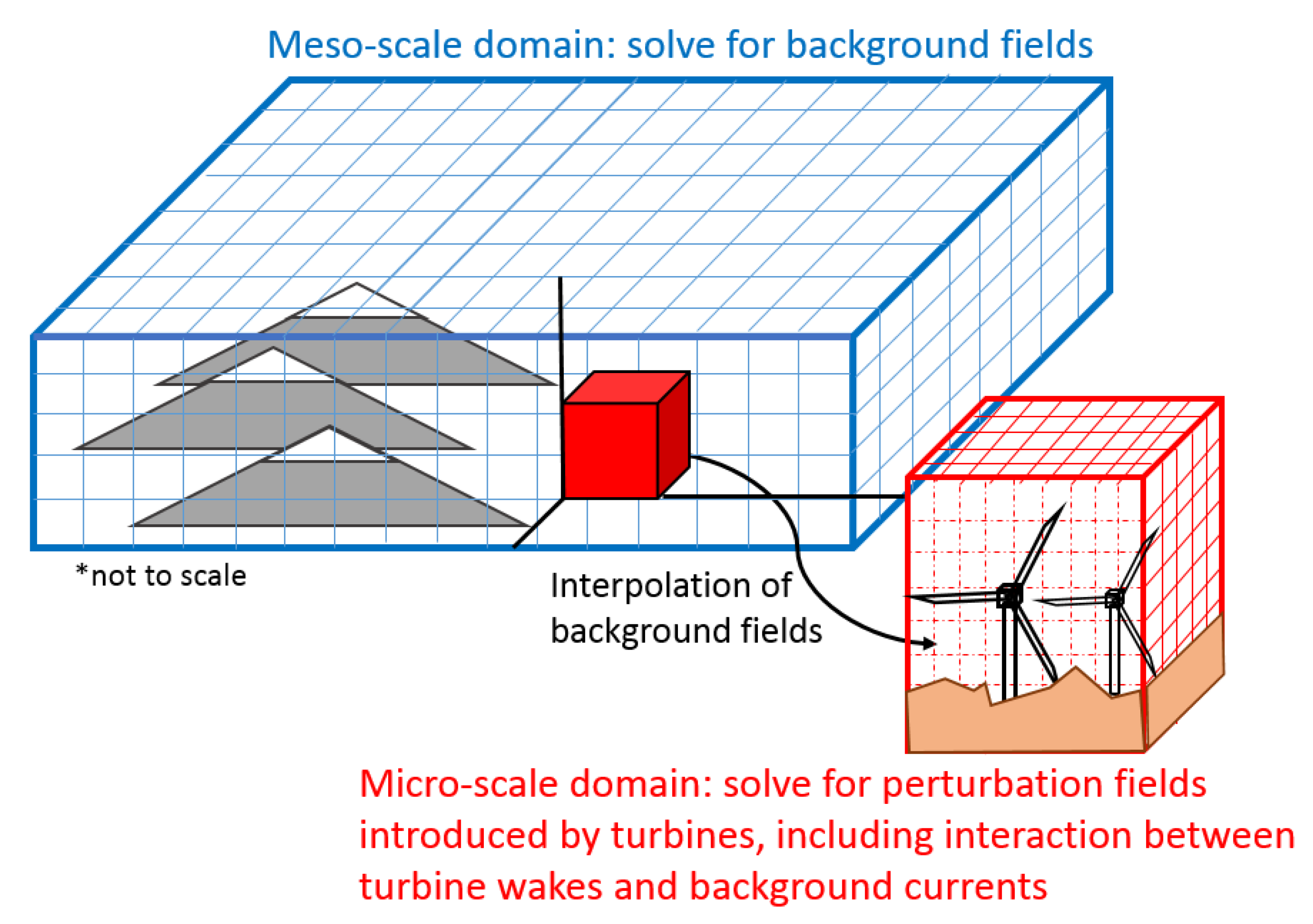
4) for the background fields for each timestep, and then use this updated information to solve Equation (5) for the perturbation fields. For one-way coupled multi-scale simulations, in which a large-scale simulation is performed beforehand, one may also spatially and temporally interpolate the fields from the large-scale simulation onto the small-scale simulation as the background fields, and then simulate a perturbation on the small-scale domain. This method, as roughly shown in
Figure 1, is reminiscent to the nested simulations that are seen in multi-scale simulations at present, and may be beneficial for these types of simulations. In this way, only Equation (5) needs to be solved. Another possible method is to prescribe the background fields from an analytic or empirical expression. When assuming the timescale of the simulation is very small when compared to the timescale of the background, one may also treat the background fields as constant in time and, therefore, treat them as a function of space only.
2.1. Governing Equations
The MSLPM is applied to the governing equations of stratified turbulent flow in order to determine the equations of motion for the background fields and perturbation fields. Beginning with the incompressible unsteady Reynolds-averaged Navier–Stokes equations and a scalar transport equation for temperature
T, as given in Equations (
6)–(8), below. Here,
is the velocity vector;
, kinematic viscosity;
, Reynolds stress tensor;
p, deviation from the hydrostatic pressure;
, constant reference density;
, density of the fluid;
, gravity vector; and,
, molecular diffusivity of temperature. An eddy diffusivity model, such that turbulent diffusivity
, where
is the eddy viscosity, is used in order to close the turbulent fluxes for
T. The divergence of the Reynolds stress tensor accounts for the average affect of turbulent fluctuations on the mean flow.
The total fields are then decomposed into their background and perturbation components following the MSLPM, which results in two sets of equations, with the first set describing the motion of the background fields given in Equations (
9)–(11) and the second set describing the motion of the perturbation fields, including any non-linear interaction between the background and perturbation fields, in Equations (
12)–(14). A linear equation of state, as defined in Equations (
15)–(17), is used, where the thermal expansion coefficient of seawater
is taken as
C/m. Equation (
18) gives the Brunt–Väisälä frequency
N in terms of both density and temperature.
The buoyant
turbulence model is used in order to close the turbulent momentum fluxes [
17]. This model is an extension to the popular
model, and it accounts for the effects of buoyancy through a source term in both the
k and
equations [
18]. While this model is not the most realistic for geophysical turbulence, it was chosen for its speed in the case presented here. The model equations are given in total form in Equations (
19)–(21), with their equivalents for the background turbulence fields in Equations (
22)–(24), and the governing equations for the perturbation turbulence variables in Equations (
25)–(27). The following model coefficients are used:
,
,
,
,
,
, and
.
where
2.2. Simulation Setup
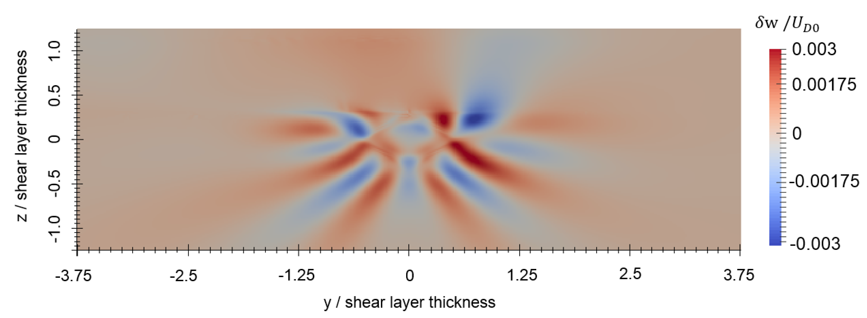
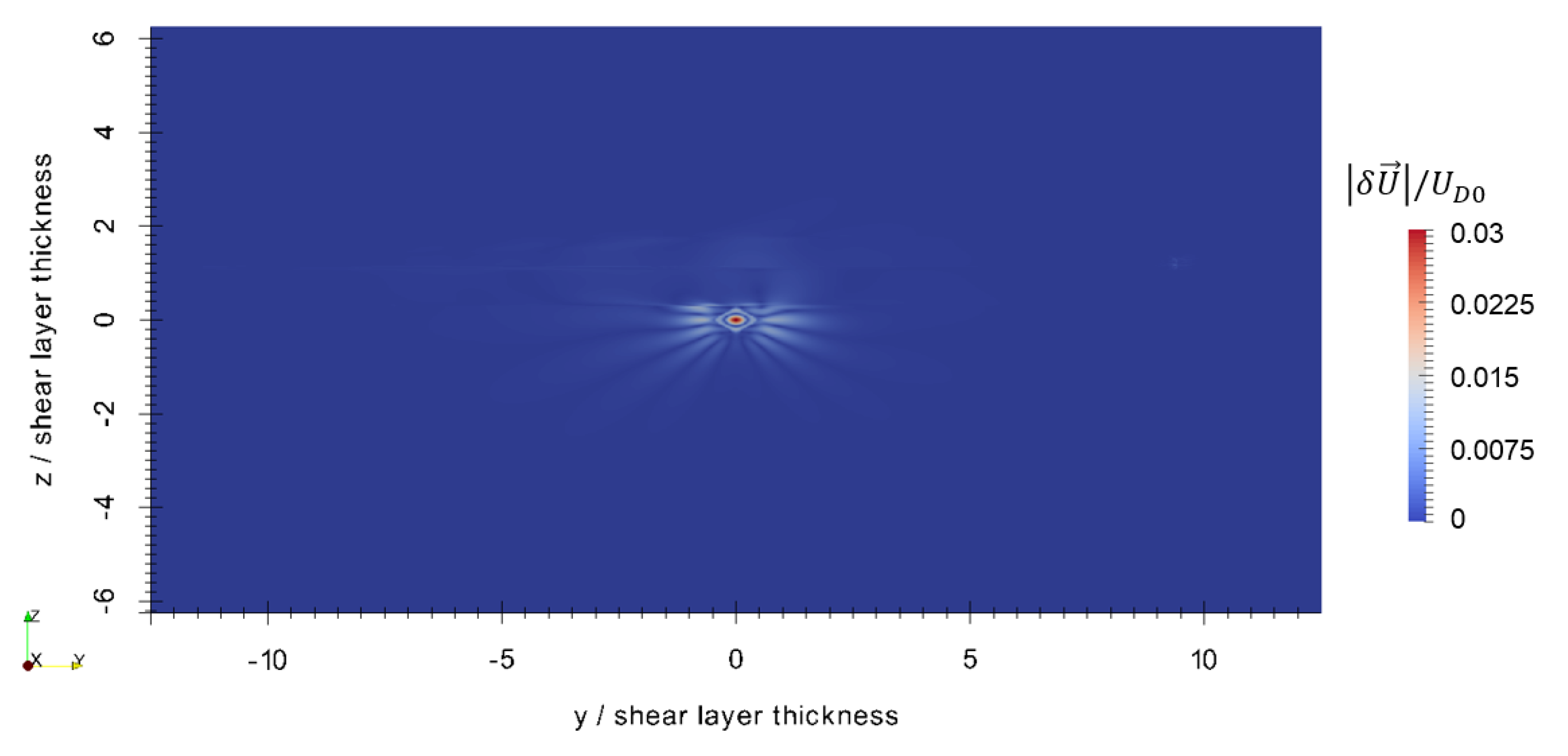
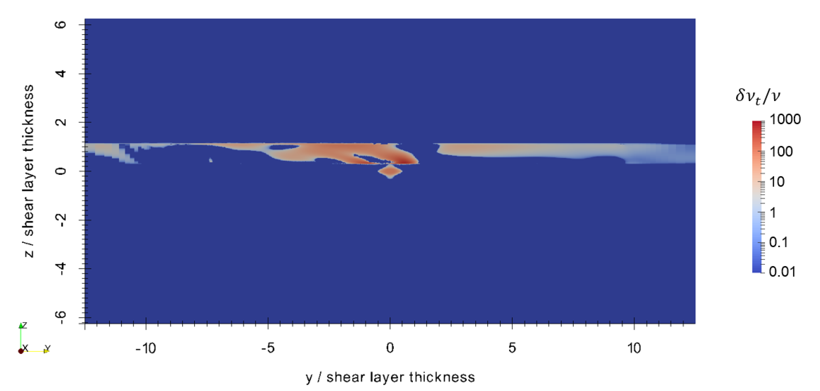
A simulation case focusing on the application of the MSLPM to a geophysical fluid flow is defined, focusing on the interaction of a perturbation with the background current. A thermally-mixed axisymmetric current is initialized as a perturbation within the computational domain, where a vertically-varying background shear layer is present. The currents are situated, such that they flow perpendicular with respect to each other. The axisymmetric current is allowed to evolve in time and, as the simulation begins, this current will collapse from buoyancy forces, forming internal gravity waves. These internal gravity waves will radiate out, with some of them reaching the background shear layer and interacting with it. Such internal gravity wave-shear layer interactions have been theoretically studied by Eltayeb and McKenzie, and numerically studied by Galmiche et al. and Javam et al. [
19,
20,
21]. It is assumed that the background shear layer is also slowly varying, such that it can be assumed to be constant in time over the span of the simulation. This case may be representative of a sewage outflow into a bay or estuary with a strong submerged current. This demonstration simulation is divided into two sections: a one-dimensional (1D) precursor simulation where turbulence fields are initialized and background fields are constructed, and then a 2D+t simulation where the axisymmetric current evolves under its own dynamics as well as influence from the shear layer. The axisymmetric current and its associated turbulence fields in the latter simulation are initialized to its respective perturbation fields, while the quantities that are associated with the shear layer are stored within the background fields. Because the background shear layer is held fixed in time, only Equations (
12)–(14) and (
25)–(27) are solved each timestep. These equations are implemented into OpenFOAM while using the methods described in [
16].
2.2.1. Precursor Simulation
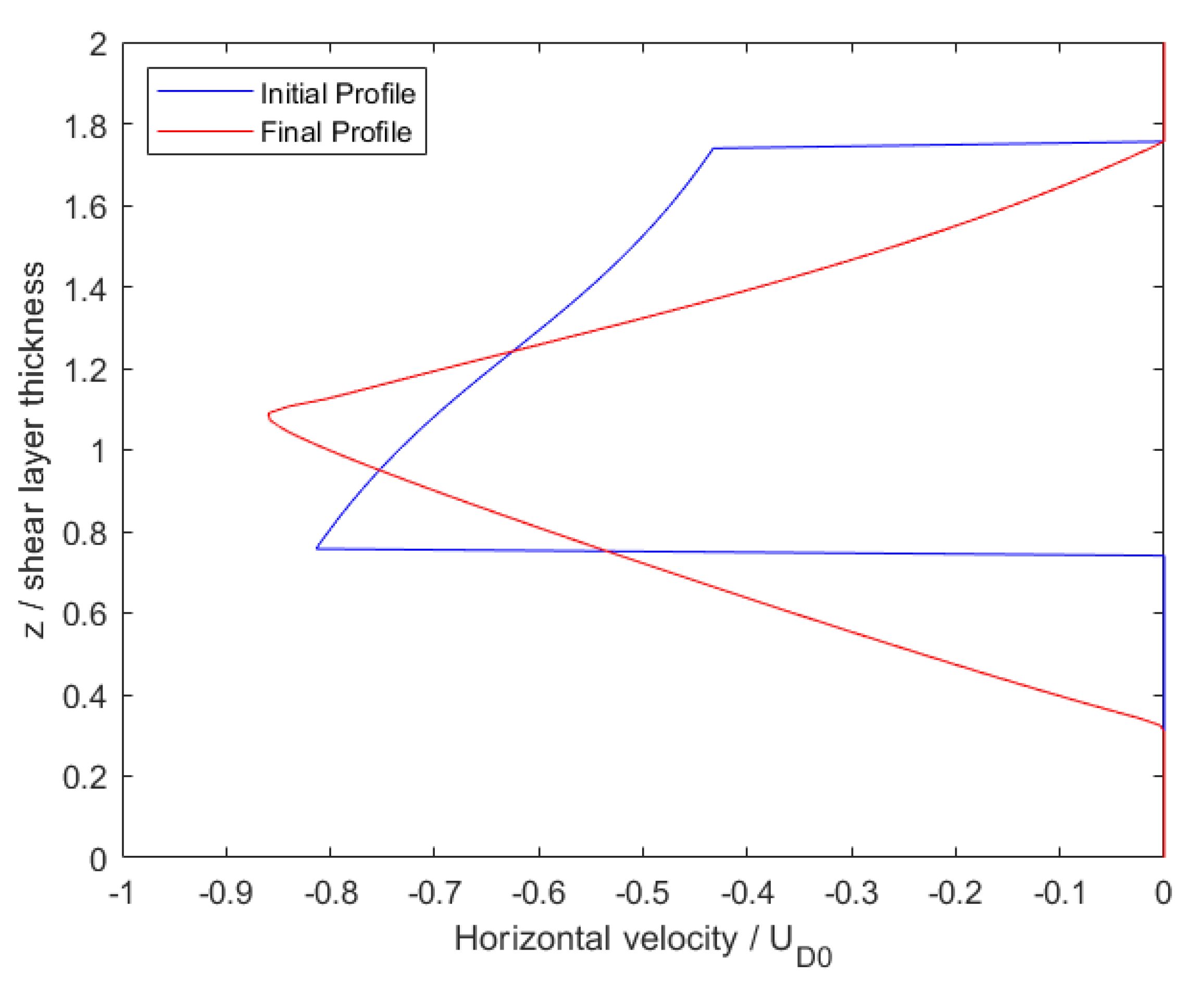
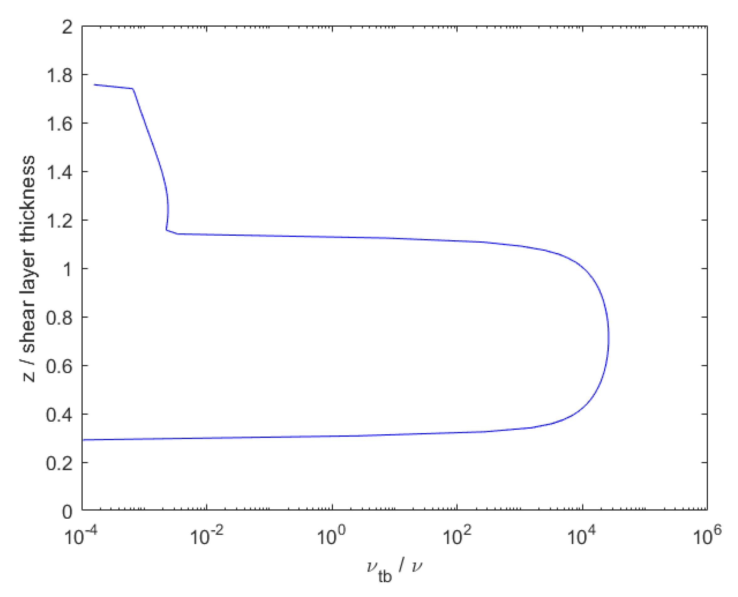
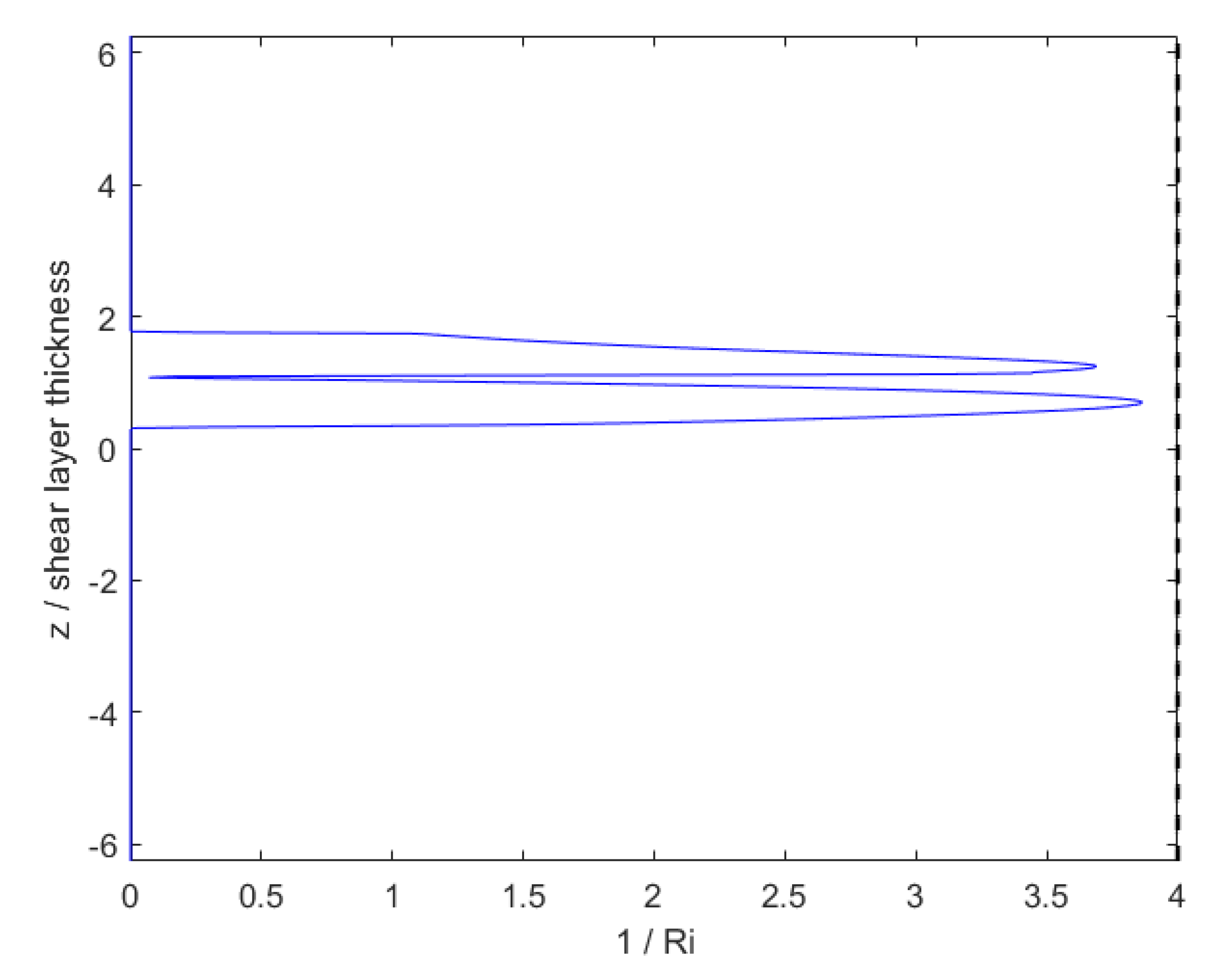
The 1D precursor simulation is performed in order to generate the background fields for the 2D+t simulation. A 500 m tall 1D domain, stretching from
z = −250 m to
z = 250 m, is discretized into 751 cells, and the simulation itself takes place over 3200 s, such that it ends when the lowest Richardson number in the domain, as defined by Equation (
28), is just above 0.25. The shear layer is initially 40 m wide and it is centered at
m, and it is initialized within this region using Equation (
29), and elsewhere the fluid is initially quiescent.
The remainder of the fields are initialized using the following equations:
N is the Brunt-Väisälä frequency and it is set at 5 cph for this simulation. is taken as 0.00505 C/m. The values for and are bounded, such that they do not decrease below the values that they are initialized at. Free-slip conditions are used on the z-normal boundaries and periodic conditions are used on the lateral boundaries.
2.2.2. 2D+t Simulation
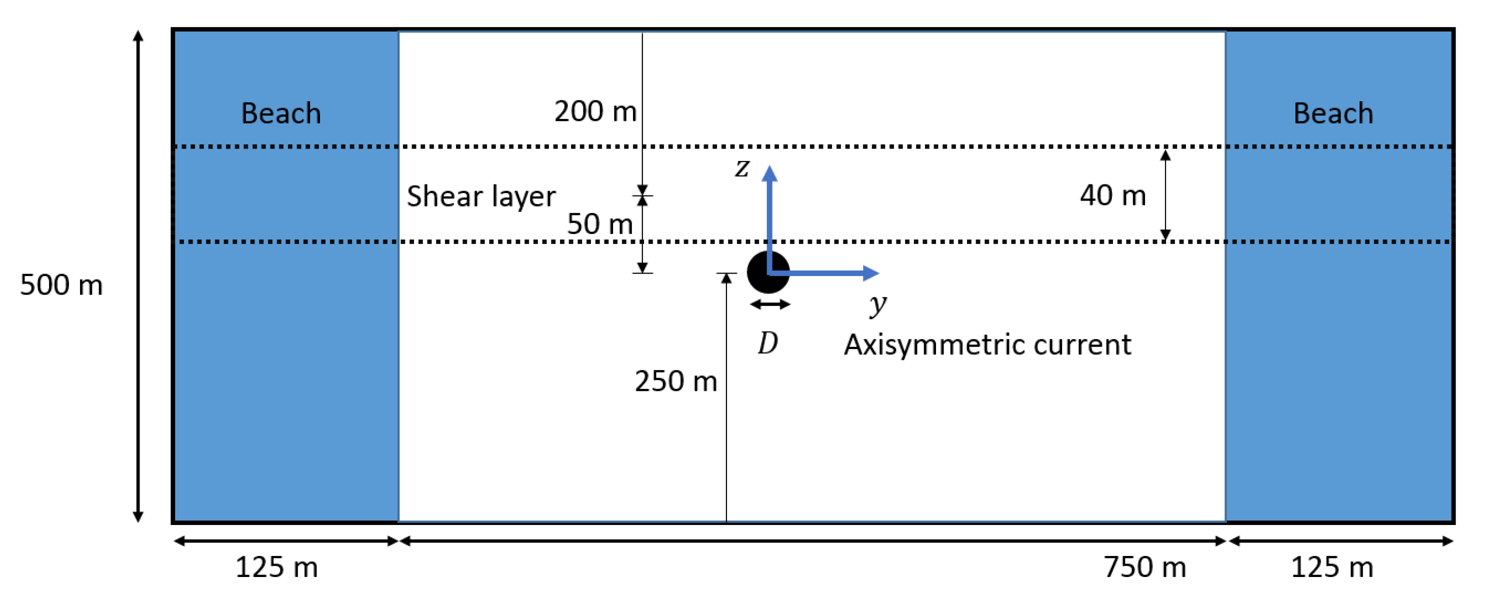
A rectangular 2D domain that is defined in
Figure 2 is used for this demonstration case, similar to the one that was used by Hassid [
22]. The 2D+t approach in this simulation can be used to approximate a steady, 3D domain while using far fewer cells than the 3D domain would nominally require, and the data periodically saved over the course of the unsteady simulation can be transformed into a third spatial dimension through a Galilean transform and a characteristic velocity
U while using
. These data can then be assembled into a 3D domain with the initial conditions located at
. The downside to the 2D+t approach is that gradients in the
x direction are lost, and so this approximation only holds if the flow slowly varies in this direction. Here, we assume that the shear layer varies in only one dimension reflective of a large-scale current, while Hassid shows that the treatment of flow that is similar to the axisymmetric current through a 2D+t application matches the experimental data well.
The domain is periodic in the x dimension, and it has a damping beach that is placed on both sides of the domain that monotonically increases in strength as it approaches the lateral boundaries. Cell size is uniform within the central, undamped portion of the domain, but, within the beach, cells progressively stretch along the y axis as they approach the lateral boundaries. The domain is discretized into one cell in the x direction, 1125 cells in the y direction, and 751 cells in the z direction.
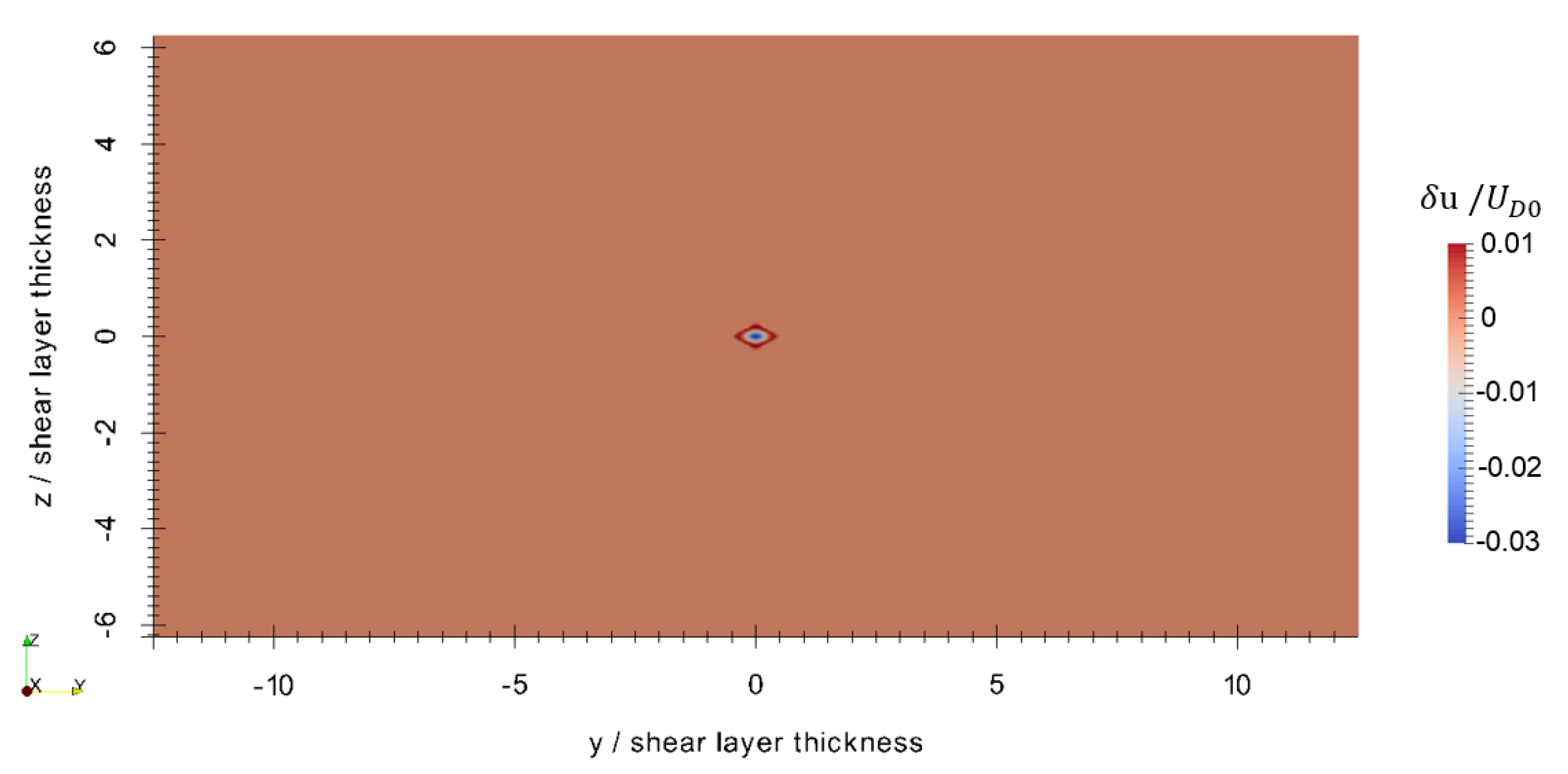
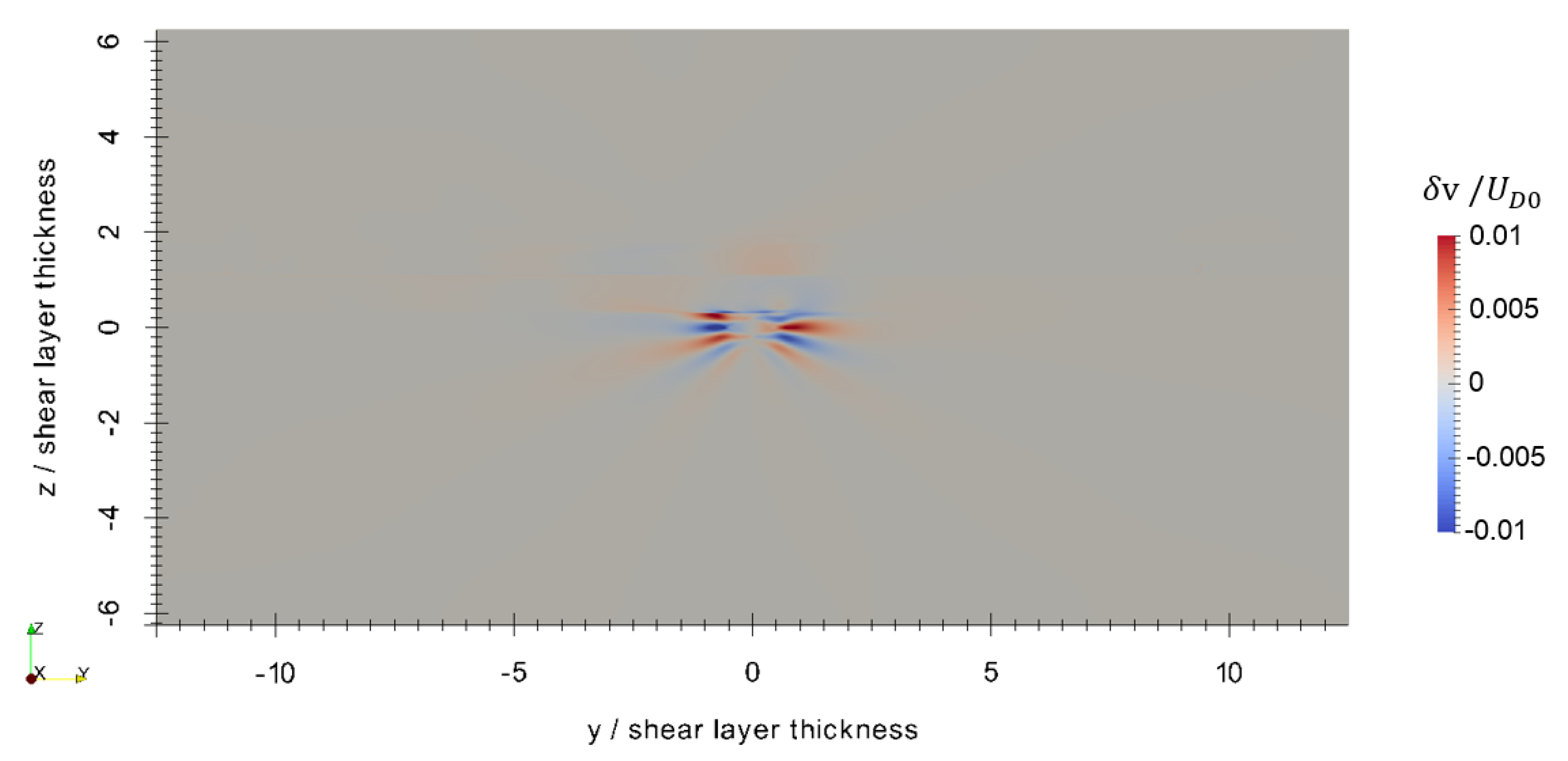
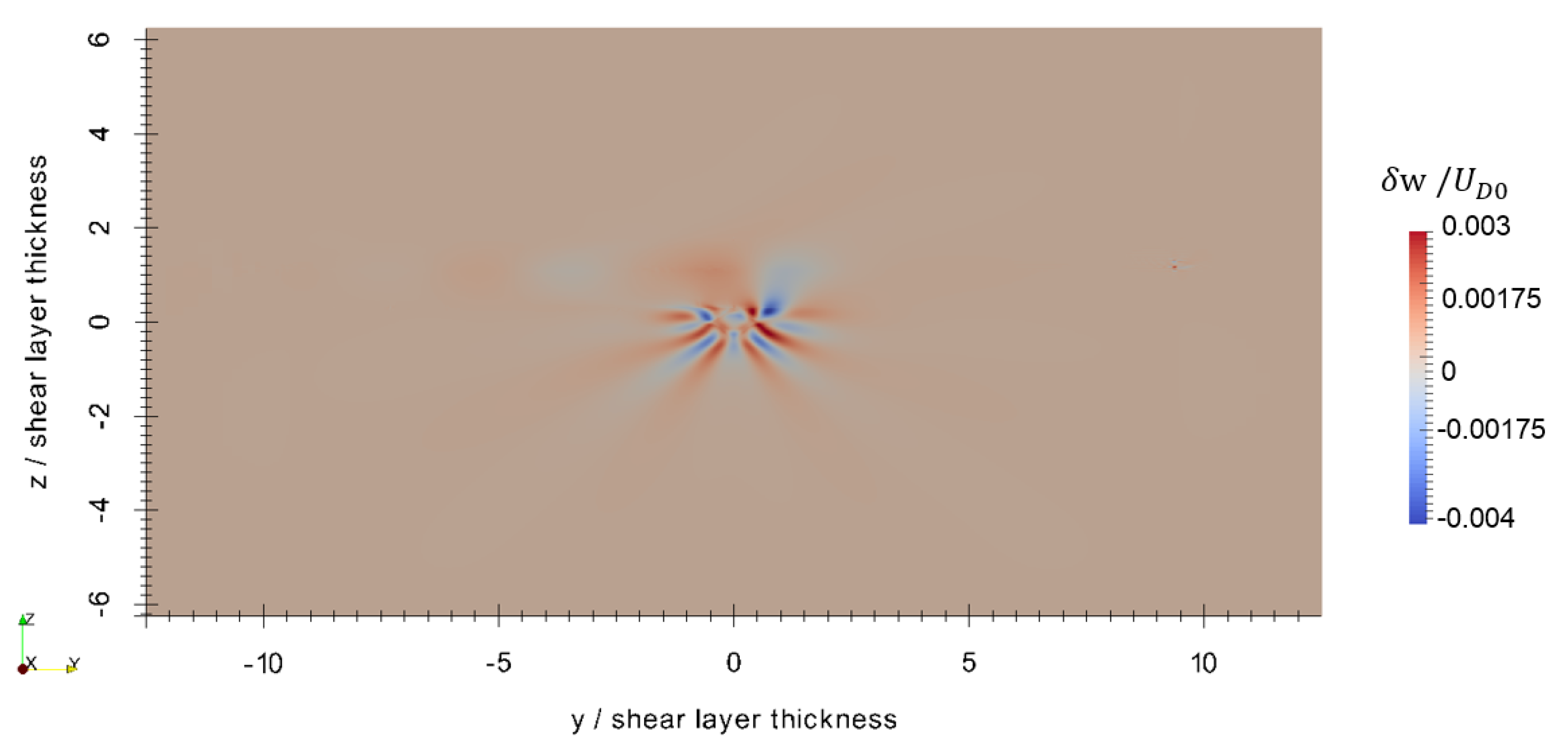
Equations (
34)–(38) are adapted from Hassid and used as initial conditions [
22]. Here,
,
,
= 1 m/s, and
D = 10 m.
Background fields are set from the results of the precursor simulation. Because only the perturbation fields are solved over the course of this simulation, no boundary conditions are needed for the background fields and, instead, their boundary values are set from the precursor simulation results. The outflow boundary conditions are used on the y-normal boundaries, free-slip conditions on the z-normal boundaries, and periodic boundary conditions on the x-normal boundaries. This simulation takes place over 3600 s.
Overall, the following assumptions were made over the course of these simulations:
the background shear current is assumed to evolve very slowly when compared to the axisymmetric current and can be modeled as evolving approximately independently of it;
the background shear current is assumed to evolve over a timescale much longer than the 2D+t simulation length, so over the course of this simulation it may be assumed fixed in time;
the background shear varies in only the vertical direction;
the axisymmetric current and any resulting internal gravity waves vary slowly in the streamwise direction; and,
the axisymmetric current and any results internal gravity waves do not have any significant impact on the evolution of the background shear current.
4. Discussion
The ability to independently track the evolution of a perturbation within an evolving background is one of the most prominent benefits of the MSLPM. Using traditional methods, several simulations may be required in order to ascertain the time history of a simulation without perturbation so that the effects of a perturbation can be determined. However, with the MSLPM, this perturbation is intrinsically separated and tracked. This benefit becomes more apparent when one must perform a series of calculations as part of a parametric study, where one may compare the evolution of a perturbation across a range of different background conditions. The separation of a perturbation from a nominal background may also yield numerical benefits, as linear solvers may be determining a solution based around zero rather than the conditions of the background state.
In the simulation documented here, a time-constant background field is defined within the domain and the perturbation allowed to interact with it. This is done without the need for boundary conditions or body source terms, which may be of interest in stratified fluid cases. The generation of internal gravity waves that radiate in all directions may result in internal gravity waves impinging on the upstream boundary, and the use of an inlet boundary condition on this same surface may lead to the reflection of waves back into the domain. Localizing the internal gravity waves to the perturbation allows for the user to place an inlet boundary condition on the background flow, then a sponge layer and an open boundary condition may be placed upon the perturbation fields in order to prevent any waves from reflecting back into the domain.
Furthermore, as the background is imposed upon the domain while using data that were collected from a precursor simulation, the influences acting upon the background can be retained, even if they are not resolved within a small-scale simulation. While it is not seen here, one could ensure that the background evolves over a certain scale. This may be important for multi-scale simulation. For example, a large-scale simulation examining continental wind patterns may examine how an upstream mountain range affects a potential downstream site, which is the subject of a small-scale simulation. This smaller-scale simulation may utilize the large-scale simulation data as a set of initial conditions, but, once the information is localized to the small-scale domain, it loses any influences of far-upstream or far-downstream phenomena which may be important. A possible remedy for this is to couple the two simulations together, which is done by the MSLPM.
4.1. Limitations of Assumptions
The MSLPM is derived under the assumption that there is sufficient scale separation between the background and perturbation, and that the perturbation does not have a significant influence upon the background. This assumption limits the perturbations that may be studied, for example, a large temperature or velocity perturbation to the entire domain, as these perturbations may have a significant impact on the dynamics of the background. Because the one-way coupling of the background and perturbation is the result of this assumption, the implementation of two-way coupling may partially relax this assumption and permit a greater range of perturbations to be studied.
Certain solution methods may also limit the applicability of the MSLPM. The case that is described in
Section 2 and
Section 3 above assumes that the time scale of the background processes is so large compared to the simulation duration that the background can be assumed to be constant in time. This requirement may be restrictive, depending on the background flow used, but two other solution methods are described in
Section 2. The simultaneous solution of background and perturbation fields on the same domain may also be used for this case and, in particular, may have been more appropriate given the nature of the background shear flow. Interpolating the background fields temporally and spatially from a separate simulation could also be used. This method may be of interest to nested multi-scale simulations; however, one must ensure that proper interpolation is used.
The 1D and 2D+t simulations were also conducted under the assumption that the flow evolves slowly in certain directions. The 1D simulation was performed in order to provide initial conditions for the background shear in the 2D+t simulation, and as such it loses any evolution in other directions, particularly the
y direction in which it flows. Within the 2D+t simulation, any significant changes in the direction in which the axisymmetric current flows is lost. While this mainly affects the evolution of the axisymmetric current, the interactions between internal gravity waves and the background shear layer may lose any 3D effects that may be important in the interactions. Similarly, the choice of a
type model may also affect the quantitative values that are seen in
Figure 6,
Figure 7,
Figure 8,
Figure 9 and
Figure 10. In this case, the results seen here may only be qualitatively correct. As a final note, this case is demonstrative of the capabilities of the MSLPM, so no quantitative conclusions should be drawn from these results.
4.2. Future Work
Further cases with more diverse phenomena and physics may be useful in order to better quantify the capabilities of the MSLPM relative to traditional simulation methods. In particular, the different solution methods that are described in
Section 2 may be tested, as these will give researchers the ability to fine-tune their simulation for the given background flows of interest. Further benchmark cases may be useful in understanding which background solution method is most practical for different flows and phenomena. Two-way coupling of the background and perturbation fields may also be of interest in order to allow for the perturbation to affect the evolution of the background. This is particularly relevant to turbulence quantities, as the great range in temporal and spatial scales of turbulent motion means that scale overlap is nearly guaranteed. While the methods that are described in this paper are in their infancy, they show great promise for geophysical flows, including multi-scale simulation of geophysical flows and, potentially, other realms of computational physics.


