Abstract
The results from a temporal linear stability analysis of a subsonic boundary layer over a flat plate with a straight and wavy leading edge are presented in this paper for a swept and un-swept plate. For the wavy leading-edge case, an extensive study on the effects of the amplitude and wavelength of the waviness was performed. Our results show that the wavy leading edge increases the critical Reynolds number for both swept and un-swept plates. For the un-swept plate, increasing the leading-edge amplitude increased the critical Reynolds number, while changing the leading-edge wavelength had no effect on the mean flow and hence the flow stability. For the swept plate, a local analysis at the leading-edge peak showed that increasing the leading-edge amplitude increased the critical Reynolds number asymptotically, while the leading-edge wavelength required optimization. A global analysis was subsequently performed across the span of the swept plate, where smaller leading-edge wavelengths produced relatively constant critical Reynolds number profiles that were larger than those of the straight leading edge, while larger leading-edge wavelengths produced oscillating critical Reynolds number profiles. It was also found that the most amplified wavenumber was not affected by the wavy leading-edge geometry and hence independent of the waviness.
1. Introduction
The aerodynamic, hydrodynamic, and acoustic performance of an airfoil with a wavy leading edge (LE) has been a subject of research for the past 30 years. This airfoil geometry was inspired by the pectoral fin of a humpback whale (Megaptera novaeangliae), which features large LE protuberances that are presumed to aid in maneuverability. One feeding behavior of a humpback whale involves swimming in circles of relatively tight radii to create a bubble net, corralling prey for efficient consumption. This banking maneuver is efficiently performed if the pectoral fin has a large stall angle combined with increased lift and decreased drag to reduce energy expenditure. Each of these performance characteristics has been investigated in the literature. Early studies of a humpback whale pectoral fin with LE protuberances were performed by Bushnell and Moore [1], Fish and Battle [2], and Miklosovic et al. [3], which suggest that the protuberances improve hydrodynamic maneuverability by increasing the stall angle and flattening out the lift curve, at the expense of reducing the maximum lift. Drag reduction was also observed due to LE tubercules. Parametric experiments by Johari et al. [4] and aerodynamic modeling by van Nierop et al. [5] were performed for several sinusoidal LE amplitudes from 2.5% to 12% chord and two wavelengths of 25% and 50% chord. These studies showed that increasing the LE amplitude increases the stall angle, while changing the LE wavelength between the two values tested had little effect on performance. Further experimentation performed by Hansen et al. [6] tested more amplitude and wavelength configurations than previous researchers, and also compared the performance of two different airfoils. The wavy LE was more effective on the airfoil that best matched the humpback whale pectoral fin cross-section. The LE wavelength data suggest that design optimization is necessary, where smaller wavelengths at or below 15% chord showed improvements in all the flight metrics of the maximum lift and stall angle, drag reduction, and post-stall characteristics, while the largest 60% chord wavelength showed no appreciable benefits over the straight LE airfoil. It is also noted that the performance can be negatively affected if the wavelength is too small. Thus, there are a range of amplitude and wavelength combinations that have advantages over the straight LE airfoil.
While measurements have confirmed the aerodynamic benefits of LE protuberances, the physical mechanism behind the performance characteristics has been described in various ways by researchers. Analogies were initially drawn to vortex generators [2,3], which enhance momentum exchange within the boundary layer and tend to keep the flow attached along more of the chord. Later studies of Hansen et al. [6] support the vortex generator description, reporting that airfoil design with a wavy LE is similar to optimizing vortex generators. The theoretical treatment by van Nierop et al. [5] proposed that the LE protuberances do not act as vortex generators due to their size relative to the boundary layer, and instead that the wavy LE modifies the airfoil pressure distribution. This leads to a pressure minimum at the trough, resulting in local separation, causing stall only over portions of the airfoil, which contributes to flattening the lift curve. Favier et al. [7] performed a direct numerical simulation of a stalled airfoil, and proposed that a Kelvin–Helmholtz instability may be responsible for streamwise vorticity that delays separation.
Acoustic studies of Hansen [8], Zhang and Frendi [9], and Biedermann and Czeckay [10] all point to larger amplitudes and smaller wavelengths as having the best noise reduction characteristics. Zhang and Frendi [9] performed scale resolving RANS-LES computations of an airfoil in the subsonic wake of a circular cylinder. The LE geometry of a 24% wavelength and 20% amplitude was found to break up the incoming vortex and channel it down the trough of the LE wave. They also found a 4 to 10 dB noise reduction at various locations in the far field, especially near the wavy leading edge. Biedermann et al. [10] performed measurements in an aeroacoustic wind tunnel for a range of LE wavelengths and amplitudes, finding local noise differences of up to 12 dB, and also confirming that the best acoustic performance occurs for small wavelengths and large amplitudes of 7.5% and 45% of chord, respectively. These studies show that LE waviness has the capability to be a passive airfoil modification that has both acoustic and aerodynamic benefits. Multiple studies [6,7,8,9] have investigated the flow structures along the airfoil, showing that the LE waviness channels turbulent structures through the trough, both accelerating them and breaking up large spanwise coherent structures and concentrating vorticity within the trough. Thus, the boundary layer is modified by the wavy LE, possibly adding an element of passive boundary layer control to the wavy LE benefits.
There is extensive literature on two- and three-dimensional boundary layer stability and control. Early work on two-dimensional stability was performed for a perfect fluid by Rayleigh [11], who identified that an inflection point in the velocity profile is necessary for inviscid instability. The perturbed Navier–Stokes equations were studied independently by Orr [12] and Sommerfeld [13], resulting in the eponymous fourth-order linear ordinary differential equation (ODE) that has been widely studied. Further advancement was facilitated by efficient solutions of the fluid velocity field using the boundary layer theory of Prandtl [14], who simplified the Navier–Stokes equations to a set of parabolic partial differential equations (PDE), and further simplification by Blasius [15] produced a nonlinear self-similar ODE with the Reynolds number as the only parameter. The Blasius equation has subsequently been used in stability analyses for decades. Prandtl [16] further confirmed through experiments the existence of a viscous instability. The theory of Tollmien [17], Schlichting [18] and experiments of Schubauer and Skramstad [19] confirmed the existence of laminar boundary layer oscillations on a flat plate, later known as Tollmien–Schlichting (T-S) waves. Squire [20] identified that the minimum critical Reynolds number for a two-dimensional parallel flow with traveling T-S waves occurs in the direction of the free stream. Various numerical methods were developed to solve for the eigenvalues and eigenfunctions of the two-dimensional stability problems using the Orr–Sommerfeld equation, e.g., those of Kaplan [21], Jordinson [22], and Mack [23]; the benchmark solution for the stability of the Blasius boundary layer by Grosch and Orszag [24]; the power series methods by Itoh [25]; and the methods based on compound matrices by Ng and Reid [26].
Fluid stability research can be treated theoretically using linear stability analysis (LSA), parabolized stability equations (PSE), and direct numerical simulation (DNS). The LSA can identify stable, unstable, and neutrally stable disturbances; estimate the critical Reynolds number and the most amplified disturbances; and calculate the disturbance eigenfunctions. PSE incorporate fewer simplifying assumptions and are thus more accurate at the cost of increased complexity. DNS has been used to observe transition numerically by using unstable eigenfunctions obtained from LSA or PSE. Further research has been conducted into secondary instability resulting from saturation of the linear mode and the transition to turbulence [27,28,29].
Three-dimensional boundary layer stability generally requires the analysis to include a crossflow velocity component perpendicular to the local freestream vector. For a flat plate or airfoil, sweep and the presence of a favorable pressure gradient in the chord direction produce a crossflow velocity component. Crossflow disturbances arise as stationary and traveling waves across the span of the surface and can result in earlier transition than chordwise instabilities. A theory for three-dimensional boundary layer stability has been developed by Gregory et al. [30] and Malik et al. [31] for the rotating disk, along with Mack [32] and Nitschke-Kowsky and Bippes [33], among others. Researchers have also used simplified base flow profiles such as the self-similar Falkner–Skan–Cooke [34,35,36] family of solutions over a swept yawed wedge to approximate a three-dimensional laminar boundary layer with a favorable pressure gradient over a swept flat plate [33] and swept wing [37].
Crossflow instabilities have been observed experimentally by Arnal et al. [38], Bippes et al. [39], and Nitschke-Kowsky and Bippes [33], and others. In the 1990s, four research organizations established programs to study crossflow instabilities experimentally and theoretically: the German Aerospace Center (DLR) in Gottingen, Germany; Arizona State University (ASU) in Tempe, Arizona, United States; the Institute of Theoretical and Applied Mechanics (ITAM) in Novosibirsk, USSR; and the National Aerospace Laboratory (NAL) in Tokyo, Japan [40]. The work presented in this paper used the DLR data for code validation. Reviews covering advances in three-dimensional boundary layer stability are provided by Bippes [33] and Saric et al. [41].
In this study, a temporal linear stability analysis of an incompressible boundary layer over a flat plate with a wavy leading edge was performed. Both a zero-sweep and a 42.5° swept plate were considered. Parametric studies of the LE amplitude and wavelength were performed for both cases. Prior to performing the wavy LE calculations, the base flow and stability code were validated against published results for Blasius flow for the zero-sweep case, along with a comparison with measurements performed on a swept flat plate at the DLR [40]. The infinite span swept plate geometry and freestream conditions were made equivalent to the DLR experiment. Only stationary disturbances in a three-dimensional boundary layer over the swept plate were studied, as these are considered to be characteristic of the flight environment [42]. For the zero-sweep flat plate, the same freestream conditions as for the swept plate were used, but with a zero pressure gradient in the chord direction, resulting in traveling T-S instabilities.
In the following sections of this article, the general three-dimensional mathematical model for the boundary layer velocity profile calculations and linear stability equations are presented, followed by the code validation and parametric studies of wavy and straight LEs for both a flat plate with zero sweep and that with 42.5° sweep.
2. Materials and Methods
The geometry, mathematical models, and solution methods for the temporal linear stability analysis and base flows are presented in this section. The stability equations were derived in three dimensions following the analysis of Mack [29]. The base flow solutions were obtained from the incompressible three-dimensional boundary layer equations (BLE) as well as self-similar solutions to the Blasius and Falkner–Skan–Cooke (FSC) equations.
2.1. Geometry
The geometry for the general case of a swept flat plate is shown in Figure 1. For the swept plate with crossflow velocities, two coordinate systems are used, one a body fixed system in the chord and span directions xc and yc, and a second a rotated coordinate system xs and ys, shown rotated in line with the local streamline. For the simplified case of zero sweep, the velocities are only in the chord direction and the rotated coordinates are not used. The geometry for a swept flat plate with a wavy leading edge is shown in Figure 2. The plate chord is set to c = 0.5 m to match the DLR experimental conditions, with the amplitude, A, and wavelength, λ, of the sinusoidal profile defined as a percentage of the chord. The peak of the LE wavelength is located at λ, and the trough is at 1.5 λ. The stability results for the swept flat plate are presented in terms of the 99.9% boundary layer thickness Reynolds number. The results for the zero-sweep case are presented in the nondimensional variables typically used in the Blasius equation. To ensure an equivalent wetted surface area of the flat plate with straight and wavy LEs, the chord for the wavy LE was extended by a length equal to one half of the LE amplitude A. All the chord fractions for the wavy LE plate were normalized using a chord equal to c + A/2.
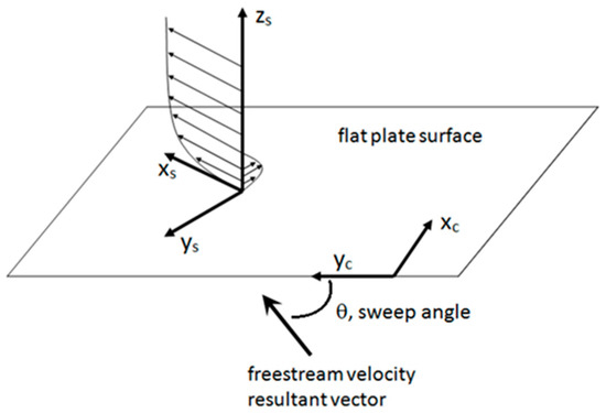
Figure 1.
Flat plate coordinate system geometry. The flat plate is shown with straight leading edge, and typical streamline and crossflow velocity profiles are shown on the rotated coordinates.
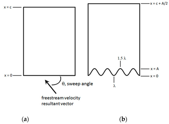
Figure 2.
Geometry of flat plate with (a) straight leading edge (LE) and (b) wavy LE.
2.2. Linear Stability Equations
The solution method for the three-dimensional linear stability equations follows Mack [29]. The nonlinear perturbation equations were derived from the nondimensional incompressible Navier–Stokes equations,
by introducing the perturbed velocities and pressures, , and subtracting the original non-perturbed equation. Here, are the fluid velocities in the x, y, z coordinates, respectively, with the z coordinate across the shear layer. The Reynolds number is R; p is the pressure; are the local base flow velocities and pressure; and are the perturbation velocities and pressure. The boundary layer thickness and the local freestream velocity were used as the reference length and velocity scales, respectively. By assuming small disturbances and a locally parallel base flow, the equations were simplified to a linear and separable system of partial differential equations. This allows the use of a separable function for the disturbances,
where are the disturbance amplitudes corresponding to , respectively; and are disturbance wavenumbers in the x and y directions, respectively; and is the frequency. For the temporal analysis, the frequency is a complex number, where the imaginary component is the amplification factor. The amplification factors can be positive, zero, or negative, indicating an unstable, neutrally stable, or stable disturbance, respectively. Substituting (2) into the linearized, separable perturbation equations gives the nondimensional continuity and momentum perturbation equations, now a system of ordinary differential equations:
In Equation (3), the prime, ′, and double prime, ″, indicate first and second derivatives with respect to z, respectively. The boundary conditions for Equation (3) are no slip at the wall,
and that the disturbances go to zero in the freestream,
The shooting method was used to satisfy the flat plate boundary condition and solve iteratively for the eigenvalues. The compound matrix method of Ng and Reid [26,43] was used to relieve the stiffness of the equations.
2.3. Base Flow Models
Solutions of the Blasius equation, the FSC equations, and the three-dimensional incompressible BLE were used as the input to the stability code. Similarity solutions of the Blasius and FSC equations for a straight LE plate were used for the validation of the stability code for swept and un-swept plates.
The FSC equations can be used to approximate an infinite span swept flat plate with a favorable pressure gradient and straight LE, with the pressure gradient controlled by the dimensionless Hartree parameter βH and the three-dimensionality controlled by the local sweep angle . The chordwise and spanwise components of the FSC model flow are
and the functions and are the solutions to the following FSC equations:
with boundary conditions
In the above equations, and are the chord and span velocities, respectively. It is noted that setting results in the Blasius equation. The FSC equations were solved using the shooting method, where the freestream boundary conditions were met by iterating on the unspecified initial conditions and to drive and to unity.
The boundary layer approximation to the incompressible Navier–Stokes equations for steady flow is given in Equation (9). These are parabolic equations and can be marched in the chord and span directions with the known free stream velocities and and specified initial conditions. For an infinite span flat plate, the flow is three-dimensional, but its velocities are independent of the span-wise coordinate y; hence, the bracketed terms in Equation (9) are neglected.
Equation (9) is subject to the following boundary conditions:
For the wavy LE plate, free boundary conditions in the plane of the plate surface were applied when the flow was in between LE peaks and not contacting the plate surface. The BLE were solved using an implicit finite difference discretization and uniform grid, with the tri-diagonal matrix algorithm for matrix inversion [44].
3. Results
This section begins with the validation of the base flow and stability calculations by comparison with published numerical solutions and experimental data. After the base flow, the stability results for a zero-sweep and swept flat plate are presented. Most of our results are presented in nondimensional variables unless otherwise specified. For the wavy leading-edge plate, a uniform notation is adopted similar to that found in the literature [8,9,10] to indicate the wavelength and amplitude of the waviness. For example, “aAwW” means a% chord Amplitude and w% chord Wavelength with a and w varying between 0 and 40 in this paper. As an example, a 10A30W wavy leading-edge plate indicates a 10% chord amplitude and a 30% chord wavelength. A straight leading edge is represented by “00AwW”, indicating a 0% amplitude and any wavelength. In addition to these wavy leading-edge notations, the notation “aAwW lL” is also used to indicate the spanwise integration extent. Namely, “10A30W 2L” refers to 10% chord amplitude and 30% chord wavelength integrated to two wavelengths.
3.1. Base Flow Validation
The FSC equations, infinite span BLE, and full 3-D BLE integrations were first solved for the case of a zero pressure gradient and a 45° swept plate, with all the results matching published values for the Blasius profile. Next, the FSC and infinite span BLE were compared to experimental data from the DLR [33] for a swept plate with a strong favorable pressure gradient, at an 80% chord location. An effective sweep angle of 42.5° was used in the calculations based on the DLR data. For the BLE code, the spanwise flow component of the freestream velocity was set to a constant 13 m/s, and the freestream velocity component in the chord direction increased linearly from 4.9 to 19.1 m/s to match the measured velocity gradient. Fischer and Dallmann [45] provide values for the FSC parameters from 10% to 90% chord, which were used to set up the FSC code. The infinite span BLE code requires an initial velocity profile to begin the marching procedure. The initial conditions at 10% chord were provided from the FSC integrator and marched forward in the BLE code to 80% chord. Figure 3 and Figure 4 show the comparison of the experimental and calculated velocity profiles aligned with the local freestream vector. Good agreement was found between the FSC calculations of Fischer and Dallmann [45] and our results, and between the BLE integrations and experimental data.
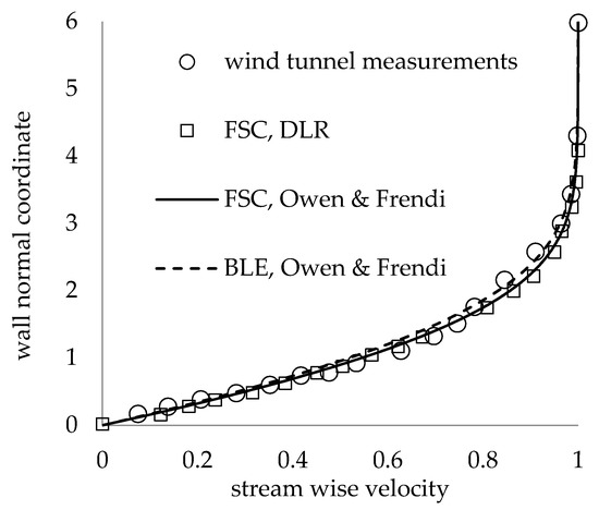
Figure 3.
Velocity profiles in the streamline direction at 80% chord.
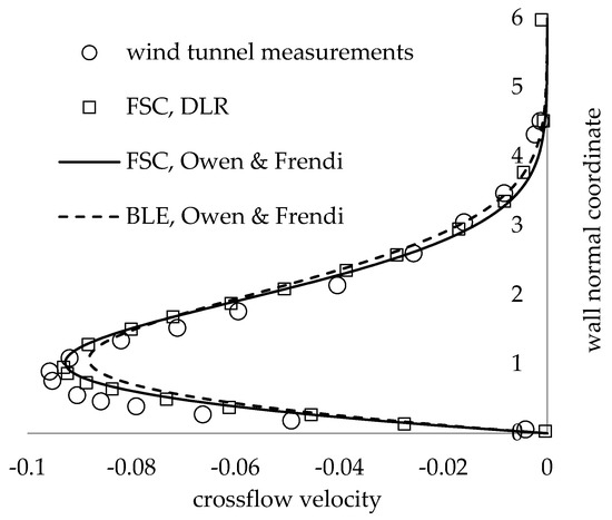
Figure 4.
Velocity profiles in the crossflow direction at 80% chord.
Next, the full 3-D BLE were compared for an infinite span flat plate with wavy and straight LEs under the DLR freestream conditions. To properly compare the infinite span straight LE and wavy LE boundary layers, the BLE for the wavy LE geometry were integrated spanwise across successive LE peaks until the flow profile at each LE peak did not change with further spanwise integration. The infinite span boundary layer profile was used as the initial condition at the wavy LE peak to start the integration. Figure 5 shows the crossflow boundary layer profiles for a wavy LE of 10% chord amplitude and 7.5% chord wavelength (10A075W) at different span locations. It is seen that the flow develops from the infinite span straight LE profile until it reaches a limiting profile at four wavelengths (10A075W 4L). Subsequent integrations to 5L and 6L show no change in the base flow profile. Furthermore, the same grid was used to integrate the infinite span solution spanwise across six wavelengths for a straight LE (labeled 00A075W 6L), and it is seen that the integration preserves the initial condition velocity profile, indicating no significant discretization errors. A similar result is found in Figure 6 for the wavy LE with a 10% chord amplitude and 30% chord wavelength (10A30W), except that the boundary layer reaches the limiting profile at one LE wavelength.
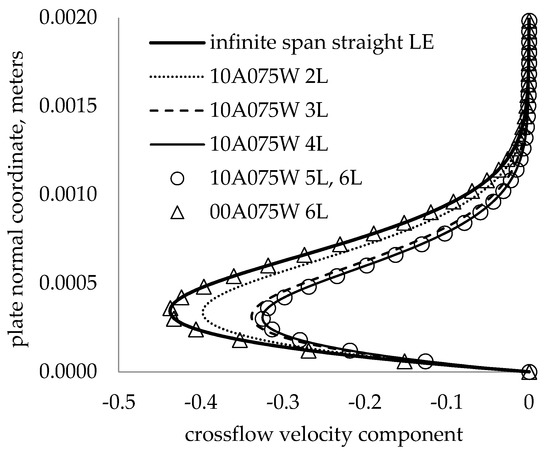
Figure 5.
Crossflow velocity profiles for straight LE and 10A075W LE at different span locations, at 20% chord.
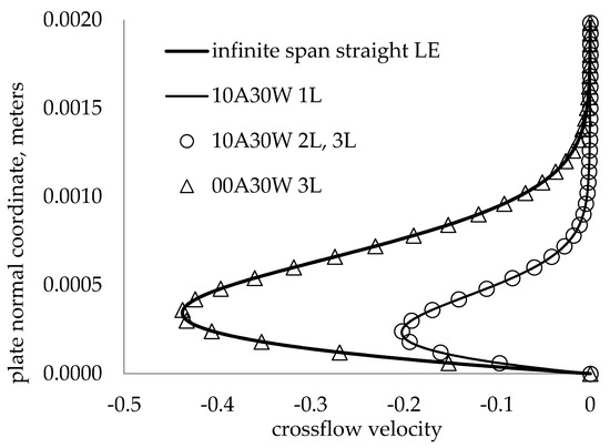
Figure 6.
Crossflow velocity profiles for straight LE and 10A30W LE at different span locations, at 20% chord.
3.2. Stability Validation
Prior to the wavy LE calculations, the stability code was validated by comparing our results with the benchmark solution of Grosch and Orszag [24] for Blasius flow eigenvalues at a single Reynolds number and wavenumber. Table 1 shows that a four-digit accuracy is achieved at a low grid resolution, and a six-digit accuracy is achieved at a higher grid resolution. Eigenvalues were also calculated at different Reynolds numbers and compared to the results from Mack [29] in Table 2, with good agreement.

Table 1.
Eigenvalues for Blasius flow at R = 580 and α = 0.179.
Table 2.
Eigenvalues for Blasius flow at different Reynolds numbers and α = 0.179.
Next, the stability equations were solved for an infinite span swept flat plate with a straight LE using an FSC base flow and compared to the experimental measurements of Nitschke-Kowsky and Bippes [33]. The most unstable stationary mode parallel to the leading edge was calculated and compared to measurements at two different wind tunnel turbulence intensities, along with published numerical solutions from Nitschke-Kowsky and Bippes [33] and Collier et al. [46], who both used FSC similarity solutions for the base flow. Good agreement among the codes and experimental data is shown in Figure 7.
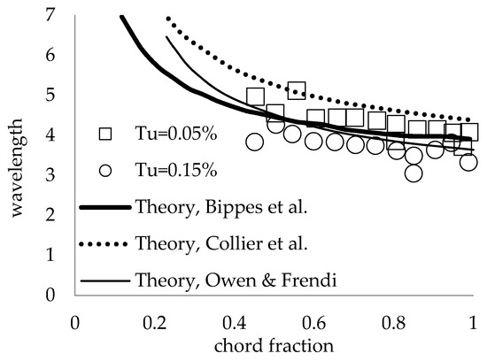
Figure 7.
Plot of the most amplified stationary wavelength parallel to the plate LE as a function of the chord fraction. Measurements shown for two different wind tunnel turbulence intensities, Tu.
3.3. Zero-Sweep Flat Plate—Base Flow and Stability
The results for the base flow and stability of the boundary layer over a flat plate with a zero pressure gradient and zero sweep relative to the freestream were calculated for a straight and wavy LE. The base flow was in the chord direction with zero crossflow, with T-S waves present in the boundary layer. The analysis began by calculating base flows for different LE geometries using the three-dimensional BLE. Insights from the base flow analysis were used to simplify the stability analysis.
3.3.1. Base Flow
For the zero-sweep flat plate, the freestream conditions used the same resultant velocity magnitude as the DLR wind tunnel experiment for a swept flat plate, with the modification of the zero pressure gradient and zero sweep, reducing the base flow to the Blasius boundary layer. For the wavy LE geometry, four parameters were varied: the LE wavelength, LE amplitude, chord location, and span location. Four different base flow studies were performed by (1) changing the span location for a fixed chord location, LE amplitude, and LE wavelength; (2) changing the span and chord location for a fixed LE amplitude and LE wavelength; (3) changing the span location, chord location, and LE wavelength for a fixed LE amplitude; and (4) changing the chord location and LE amplitude for a fixed span location and LE wavelength.
Figure 8 shows the boundary layer profiles at different span locations between the LE peaks for the straight and wavy LEs at a fixed 20% chord location, fixed wavy LE amplitude, and wavelengths of 10% and 30% chord, respectively. For the wavy LE, the boundary layer at the LE peak, labeled as 10A30W 1.0L, is identical to the Blasius profile. Deviations from the Blasius profile are seen at span locations between the LE peaks. The boundary layer thins across the span to a minimum at the trough and is symmetric about the trough.
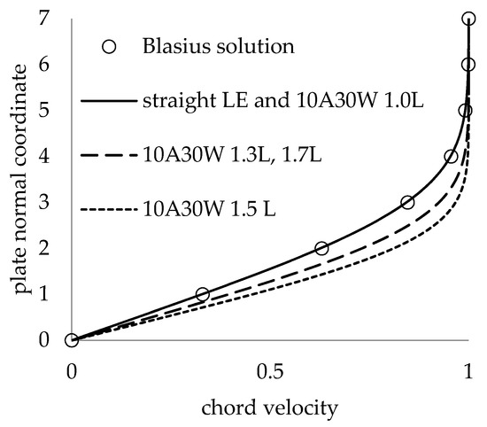
Figure 8.
Base flow profiles for different span locations at fixed 20% chord location, with 10% amplitude and 30% wavelength (10A30W). Results are shown at 1.0, 1.3, 1.5, and 1.7 λ.
The boundary layer thicknesses down the chord and at different span locations for the 10A30W wavy LE are shown in Figure 9. At the wavy LE peak, the boundary layer thickness is equivalent everywhere to the Blasius boundary layer thickness. At span locations between the LE peaks, the boundary layer is thinner and asymptotically trends toward the Blasius boundary layer thickness as the chord location is increased.
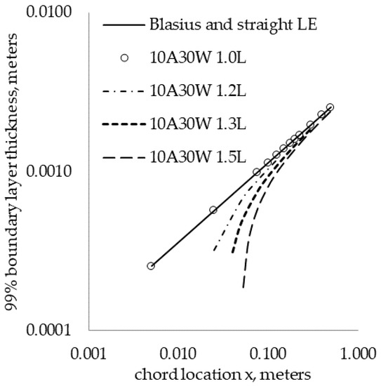
Figure 9.
Base flow boundary layer thicknesses at different chord locations.
Next, the boundary layer profiles for the wavy LE were calculated at different chord and span locations for wavelengths of 30%, 15%, and 7.5% at a fixed 10% amplitude (10A30 W, 10A15 W, and 10A075 W). It was found that the boundary layer profile plotted in both dimensional and nondimensional units at a given span location was independent of wavelength. Figure 10 shows the boundary layer thickness across the chord for three different LE wavelengths at 1.2 L and 1.5 L span locations as an example of the independence of the boundary layer profile with the LE wavelength.
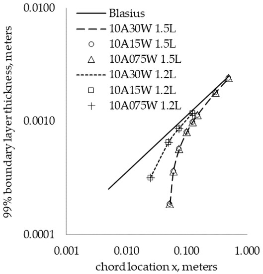
Figure 10.
Base flow boundary layer thicknesses for different leading-edge wavelengths.
Finally, the effect of the LE amplitude was investigated by calculating boundary layer profiles at different chord locations for amplitudes of 5%, 10%, and 20% chord, with a fixed 30% wavelength and fixed span location at the wavy LE trough. As shown in Figure 11, increasing the amplitude at the trough has a similar effect on the boundary layer thickness as the results in Figure 9 show; increasing the amplitude decreases the boundary layer thickness towards the LE, and the thicknesses tend towards the Blasius solution as the chord location increases.
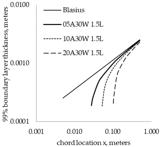
Figure 11.
Base flow boundary layer thicknesses for different leading-edge amplitudes at the wavy LE trough.
In summary, the boundary layer at the LE peak is the same as the Blasius profile and thins across the span to a minimum at the trough. The boundary layer profiles are symmetric about the trough, and the boundary layer profiles across the wavy LE span are independent of the wavy LE wavelength, while the boundary layer thins as the LE amplitude increases. Finally, the deviation of the base flow from the Blasius profile is diminished with an increasing chord location; therefore, one can conclude that the LE geometry only modifies the base flow close to the LE.
3.3.2. Stability
A parametric study of the boundary layer stability was performed for the straight and wavy LE flat plate. From the base flow results in the previous section, it was found that the LE wavelength has no effect on the base flow profile, and it was therefore not a parameter in the stability analysis. The stability results are presented in the form of neutral curves and critical Reynolds numbers, and require base flows at different chord locations. Thus, the two parameters in the stability analysis were the span location and LE amplitude.
The effect of the span location for a fixed 10% LE amplitude is shown in Figure 12. The neutral curves for the wavy LE peak and Blasius flow of the straight LE are equivalent, with a critical Reynolds number of approximately 302, which is in good agreement with Jordinson [22]. Both the critical Reynolds number and the range of unstable wavenumbers increase from the peak to the trough. The neutral curves are symmetric about the LE trough as expected from the symmetry of the base flows.
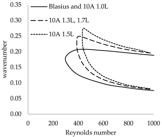
Figure 12.
Neutral curves for a fixed 10% amplitude at different span locations.
The effects of varying the LE amplitude at a fixed span location were calculated. Figure 13 shows that the effect of doubling the amplitude from 10% to 20% had a similar trend to varying the span location for a fixed amplitude, as expected from the base flow study. Both the critical Reynolds number and range of unstable wavenumbers were greater for the 20A case than the 10A case. The effects of the span location and LE amplitude on the critical Reynolds number are more clearly shown in Figure 14. The critical Reynolds number profile follows an oscillating pattern with the span location. The maximum critical Reynolds number appears at the trough and 0.5 and 1.5 wavelengths, and is increased for a larger LE amplitude.
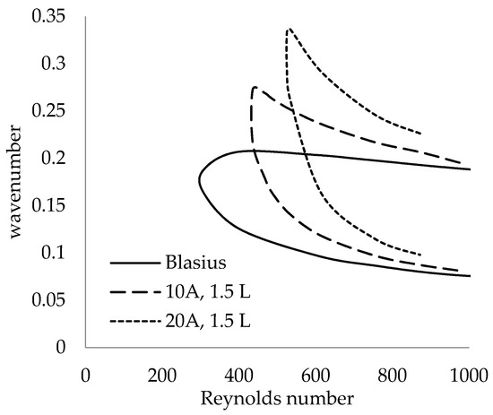
Figure 13.
Neutral curves for different amplitudes at the LE trough.
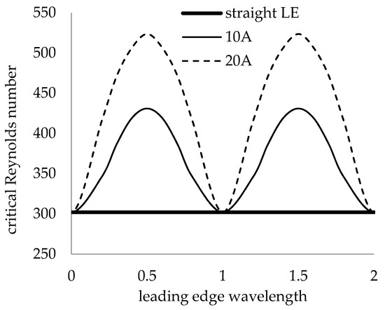
Figure 14.
Critical Reynolds numbers for different leading-edge geometries.
In summary, the stability analysis for the zero-sweep plate with a zero pressure gradient and wavy LE produced similar conclusions to those of the base flow study. The neutral curve at the LE wave peak was equal to that of the Blasius profile. Both the critical Reynolds number and range of unstable wavenumbers were increased across the span to a maximum at the trough, and the neutral curves were symmetric about the trough. The wavy LE neutral curves all tended towards the Blasius neutral curve as the Reynolds number was increased. The most general conclusion of the stability analysis is that the leading-edge wave geometry leads to an increase in the critical Reynolds number above that of the straight LE, with the trough of the LE wave having the highest critical Reynolds number.
3.4. Swept Flat Plate—Base Flow and Stability
A linear stability analysis for stationary crossflow disturbances was performed on an infinite span swept flat plate with straight and wavy LEs. The analysis was built around a DLR experiment [37] on crossflow stability using an effective sweep angle of 42.5°. The experiment considered here used a displacement body placed above a swept flat plate with a straight LE in a wind tunnel to create a strong favorable pressure gradient in the chord direction, stabilizing the T-S disturbances. The combination of sweep and a favorable pressure gradient created a crossflow within the boundary layer. In the DLR experiment, end plates were placed on the swept flat plate to approximate infinite span flow conditions along the center of the plate. A parametric study of the flat plate with a wavy LE is presented. A systematic analysis of the base flow across the wavy LE was first performed to aid in the parametric study of the boundary layer stability. The results are first presented as a local analysis at a single span location, the wavy LE peak, and then a global analysis at span locations between successive peaks.
3.4.1. Local Analysis
The fully three-dimensional BLE were solved for a swept flat plate with straight and wavy LEs for one set of freestream conditions. Calculations were performed at a single span location, i.e., the peak, for the local analysis.
The freestream velocity profiles U(x) and V(x) were chosen to match the DLR experiment, with initial U(x = 0) = 4.9 m/s. This allowed for non-zero velocities to be present everywhere in the flow, except for the plate surface, and facilitate solution by the boundary layer code without the requirement of a self-similar FSC or Hiemenz flow initial condition.
For a wavy LE, the flow profile will approach that of a straight LE plate when the LE wavelength approaches both zero and infinity. It is therefore expected that an optimum LE wavelength between zero and infinity may exist that maximizes the wavy LE modification of the base flow. To estimate the optimized LE wavelength, base flow calculations were performed over a range of LE wavelengths at a fixed LE wave amplitude of 10% chord and a fixed 10% chord location, and compared to the infinite span solution for a straight LE. Figure 15 plots the crossflow peak velocity ratio, defined as the peak crossflow velocity normal to the freestream resultant vector for a wavy LE divided by the same velocity for the straight LE. It is seen in Figure 15 that the velocity modification factor approaches unity for a zero wavelength and for large wavelengths, and that there exists a wavelength near 25% chord that minimizes the crossflow velocity.
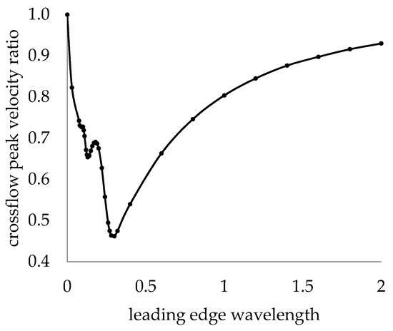
Figure 15.
Velocity modification factors at the LE peak and 10% chord location. Straight leading-edge results are shown at zero wavelength.
The stability of the wavy LE was next investigated by calculating neutral curves for different LE geometries. First, the effect of different LE amplitudes at a fixed wavelength was investigated. Based on the results from Figure 15, a wavelength of 25% chord was chosen, and amplitudes of 5%, 10%, 20%, and 40% of the plate chord were used to calculate the neutrally stable eigenvalues. Figure 16 shows the neutral curves for each case, all of which retained the same general shape. The critical Reynolds number nearly reached a limiting value at a 20% amplitude. It is noted that each neutral curve approached the straight LE neutral curve at a sufficiently high Reynolds number, and that all the neutral curves exhibited instability over a large range of wavenumbers.
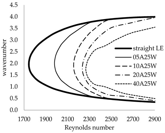
Figure 16.
Neutral curves for 42.5° swept flat plate with different leading-edge amplitudes at fixed wavelength of 25% chord, along with straight leading-edge neutral curve.
Next, the effect of different LE wavelengths from 15% to 40% chord at a fixed 10% amplitude is shown in Figure 17. The 30% chord wavelength had the highest critical Reynolds number. The 25% chord wavelength, not shown in the figure, had a similar shape and nearly the same critical Reynolds number as the 30% wavelength. The 40% chord wavelength approached the limiting case of the straight LE. Figure 18 shows the critical Reynolds number for a range of wavelengths and amplitudes. The asymptotic behavior of different amplitudes at a fixed 25% chord wavelength is evident, along with the presence of both a local and global maximum critical Reynolds number at a fixed 10% amplitude. For the local analysis at the LE peak, the effect of the LE wavelength is an optimization problem, while the effect of increasing the LE amplitude is asymptotic.
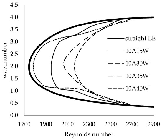
Figure 17.
Neutral curves for 42.5° swept flat plate with different leading-edge wavelengths at fixed amplitude of 10% chord, along with straight leading-edge neutral curve.
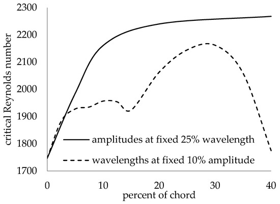
Figure 18.
Critical Reynolds numbers for different LE geometries.
Plots of the temporal amplification factor for a Reynolds number of 2300 at a fixed 10% amplitude and for a range of wavelengths are shown in Figure 19. The most amplified wavenumber is nearly constant for all the LE geometries, showing that the LE waviness has little effect on the most amplified wavenumber.
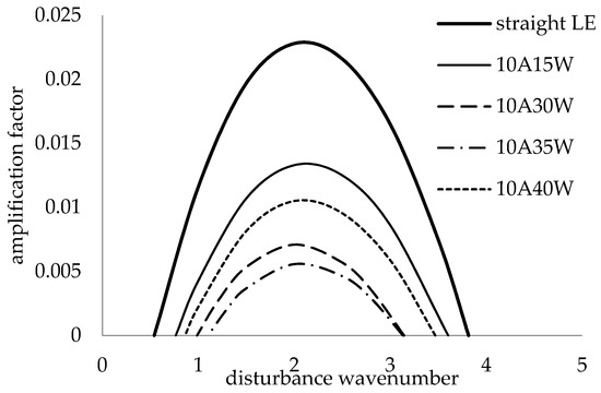
Figure 19.
Amplification curves at fixed 2300 Reynolds number.
3.4.2. Global Analysis
A global stability analysis was performed for different LE geometries by calculating the critical Reynolds numbers and maximum amplification factors at span locations between successive LE peaks. The effect of the LE wavelength is presented first. Figure 20 shows the critical Reynolds numbers for wavy LE geometries at a fixed 10% amplitude and 30%, 15%, and 7.5% wavelengths (10A30W, 10A15W, and 10A075W, respectively). The critical Reynolds numbers are plotted against a nondimensionalized LE wavelength, with integer values of the nondimensionalized wavelength corresponding to the LE wave peak, and values of 0.5 and 1.5 corresponding to the wave trough. The 10A30W geometry exhibits strong oscillations across the span, with a peak critical Reynolds number near 1.0 (the dotted vertical line shows where the local analysis was carried out, Figure 17) and 2.0 and a low critical Reynolds number at or slightly below the straight leading-edge case near 0.25 and 1.25. The effect of sweep is characterized by the steep decline in the critical Reynolds number past the peak near the wavelength of 1.0 and a slow gradual rise past the wavelength of 1.25. By contrast, for the 10A15W and 10A075W geometries, the critical Reynolds number had less pronounced oscillations across the span, with both cases having similar critical Reynolds number when averaged over the LE wavelength. Additionally, it is worth noting that the maximum critical Reynolds number for both cases—10A15W and 10A075W—occurred near the trough: wavelengths 0.5 and 1.5. On average, the critical Reynolds numbers for all three cases were higher than the straight leading-edge case.
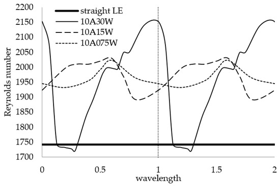
Figure 20.
Global critical Reynolds number profile for fixed amplitude and variable wavelength. The wavy leading-edge peak location is shown with the vertical dotted line.
The maximum amplification factors at a fixed 0.124 chord fraction are shown in Figure 21. This chord fraction was chosen since it was far enough down the chord that unstable disturbances were present, but not so far down the chord that the effects of the wavy LE on the base flow were diminished. The maximum amplification factor for the 10A30W geometry had an oscillating profile, with the amplification being smaller everywhere than the straight LE case. The 10A15W and 10A075W maximum amplification factor profiles were more constant and less amplified than the straight LE geometry. The 10A075W maximum amplification factor was larger in magnitude everywhere than the 10A15W case, trending towards the straight LE maximum amplification value.
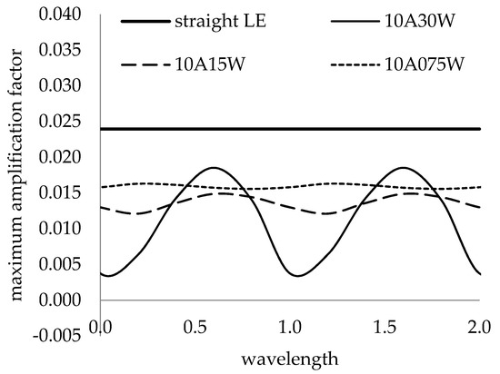
Figure 21.
Global maximum amplification factor profile for fixed amplitude and variable wavelength at 0.124 chord fraction.
The full amplification curves at a 0.124 chord fraction are shown in Figure 22 for different span locations of the 10A30W geometry and the straight LE. It is seen that the wavenumber of the most amplified mode was nearly constant at all span locations. Similar to the local analysis of Figure 19, the LE waviness had little effect on the most amplified wavenumber across the span.
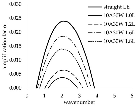
Figure 22.
Amplification curves at different span locations for 10A30W and straight LE at 0.124 chord fraction.
The global effect of the LE amplitude was calculated for 30% and 7.5% LE wavelengths. Figure 23 shows the critical Reynolds numbers for the 05A30W and 10A30W geometries. For the 5% and 10% amplitudes, the profiles oscillated across the span. Increasing the amplitude had a beneficial effect on the stability for all cases, and the maximum global critical Reynolds number was increased as the amplitude increased. Portions of the 5% and 10% amplitude cases were less stable than the straight LE geometry. Figure 24 shows the global effect of LE amplitude for the 05A075W and 10A075W geometries. Each of the 7.5% wavelength profiles were more constant along the span than the 30% wavelength profiles, and the boundary layer for the 7.5% wavelength was more stable than the straight LE everywhere for 5% and 10% amplitudes, in contrast to the 30% wavelength geometry. As the amplitude was decreased for the 7.5% wavelength case, the nearly constant critical Reynolds number profiles approached the straight LE value with little oscillation.
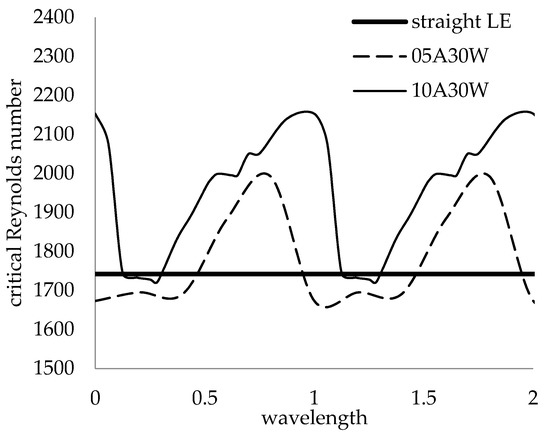
Figure 23.
Global critical Reynolds number profile for fixed 30% wavelength and variable amplitudes.
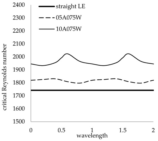
Figure 24.
Global critical Reynolds number profile for fixed 7.5% wavelength and variable amplitudes.
In summary, for the swept flat plate, the wavy LE had stability benefits verses a straight LE for a range of LE wavelengths and amplitudes. In general, the wavy LE increased the critical Reynolds number across the span and reduced the temporal amplification factor. The most amplified wavenumber was relatively constant across the span and was nearly equal to that of the straight LE. Smaller wavelengths seem to have a stability advantage, in that the critical Reynolds number was increased above the straight LE value for all the span locations and all the LE amplitudes tested.
4. Discussion
This work performed a temporal linear stability analysis for an incompressible fluid over a flat plate with a straight and wavy LE, for both zero and 42.5° sweep. The plate geometry and freestream conditions were chosen to match the experiment performed at the DLR for the swept plate analysis. The freestream conditions for the zero-sweep plate were modified from the DLR conditions by using a zero pressure gradient in the chord direction. The three-dimensional BLE were used to calculate the base flows for straight and wavy LE geometries. The disturbances for the zero-sweep plate consisted of traveling waves in the chord direction, while stationary disturbances in the crossflow direction were calculated for the swept plate. For both swept and un-swept plates, the modification of the base flow by the LE wave was most significant near the leading edge. The wavy LE base flow tended toward the straight LE base flow as chord location increased. For both the swept and zero-sweep geometries, the wavy LE resulted in higher critical Reynolds numbers and decreased the temporal amplification factor of the most amplified wavenumber at chord locations near the LE.
For the zero-sweep flat plate with a zero pressure gradient, the LE wave modified the base flow profile with respect to the Blasius boundary layer by thinning the boundary layer from the LE peak to the trough, with a minimum boundary layer thickness at the trough and symmetric boundary layer profiles with respect to the trough. The Blasius boundary layer profile occurred at the LE peak. The LE wavelength had no effect on the boundary layer profiles, while increasing the LE amplitude increased the critical Reynolds number at a fixed span location. Compared to the straight LE, the wavy LE geometry increased the critical Reynolds number and decreased the temporal amplification at all the span locations between the LE peaks, with the trough being the most stable span location.
For the swept flat plate, a local linear stability analysis was first performed at the wavy LE peak. Unlike that for the zero-sweep flat plate, the base flow for the swept flat plate was dependent on both the LE wavelength and amplitude. The effect of the LE wavelength was an optimization problem, while the effect of increasing the LE amplitude was asymptotic, with the 10A30W geometry being chosen as the most stable LE geometry at the peak since it had the largest critical Reynolds number. The most amplified wavenumber was also nearly constant and approximately equal to that of the straight LE.
A global stability analysis for the swept plate was performed at span locations between the LE peaks. In general, the wavy LE increases the critical Reynolds number across the span and reduces the temporal amplification factor. The most amplified wavenumber for the swept plate is nearly constant and equal to that of the straight LE plate across the span and chord. For larger LE wavelengths, the critical Reynolds number profiles oscillated across the span, while the smaller LE wavelengths had more constant span profiles. For a fixed LE amplitude, the largest LE wavelength of 30% chord produced the largest maximum critical Reynolds number, but due to the oscillating profile, the stability at portions of the span was the same or slightly worse than that for the straight LE. The smallest wavelengths of 15% and 7.5% chord produced more constant critical Reynolds number profiles across the span, being more stable than the straight LE everywhere. Varying the amplitude at a fixed 7.5% wavelength produced relatively constant span profiles at all amplitudes, with the average critical Reynolds number approaching that of the straight LE as the amplitude was decreased. For the 30% wavelength case, all the LE amplitudes produced an oscillating profile across the span. Amplitudes of 5% and 10% chord and a 30% wavelength had portions of the span with a smaller critical Reynolds number than the straight LE.
5. Conclusions
An extensive study of a temporal linear stability analysis for a subsonic boundary layer over a flat plate with a straight and wavy leading edge was carried out for a swept and un-swept plate. Some of the key results of this study are:
- The wavy leading edge increased the critical Reynolds number for both swept and un-swept plates.
- For the un-swept plate, increasing the leading-edge amplitude increased the critical Reynolds number, while changing the leading-edge wavelength had no effect on the mean flow.
- For the swept plate, a local analysis at the leading-edge peak showed that increasing the leading-edge amplitude increased the critical Reynolds number asymptotically, while the leading-edge wavelength required optimization.
- The global stability analysis performed across the span of the swept plate showed that smaller leading-edge wavelengths produced relatively constant critical Reynolds number profiles that were larger than those of the straight leading edge, while larger leading-edge wavelengths produced oscillating critical Reynolds number profiles.
- It was also found that the most amplified wavenumber was not affected by the wavy leading-edge geometry and hence independent of the waviness.
Author Contributions
Conceptualization, M.O. and A.F.; methodology, M.O.; software, M.O.; validation, M.O. and A.F.; formal analysis, M.O.; investigation, M.O.; resources, M.O.; data curation, M.O.; writing—original draft preparation, M.O.; writing—review and editing, A.F.; visualization, M.O.; supervision, A.F.; project administration, A.F.; funding acquisition, A.F. All authors have read and agreed to the published version of the manuscript.
Funding
This research was not funded.
Conflicts of Interest
The authors declare no conflict of interest.
References
- Bushnell, D.M.; Moore, K.J. Drag reduction in nature. Annu. Rev. Fluid Mech. 1991, 23, 65–79. [Google Scholar] [CrossRef]
- Fish, F.E.; Battle, J.M. Hydrodynamic design of the humpback whale flipper. J. Morphol. 1995, 225, 51–60. [Google Scholar] [CrossRef] [PubMed]
- Miklosovic, D.S.; Murray, M.M.; Howle, L.E.; Fish, F.E. Leading edge tubercles delay stall on humpback whale flippers. Phys. Fluids 2004, 16, L39–L42. [Google Scholar] [CrossRef]
- Johari, H.; Henoch, C.; Custodio, D.; Levshin, A. Effects of leading-edge protuberances on airfoil performance. AIAA J. 2007, 45, 2634–2642. [Google Scholar] [CrossRef]
- Van Nierop, E.; Alben, S.; Brenner, M. How bumps on whale flippers delay stall: An aerodynamic model. Phys. Rev. Lett. 2008, 100, 054502. [Google Scholar] [CrossRef]
- Hansen, K.L.; Kelso, R.M.; Dally, B.B. Performance variations of leading-edge tubercles for distinct airfoil profiles. AIAA J. 2011, 49, 185–194. [Google Scholar] [CrossRef]
- Favier, J.; Pinelli, A.; Piomelli, U. Control of the separated flow around an airfoil using a wavy leading edge inspired by humpback whale flippers. CR MEC 2012, 340, 107–114. [Google Scholar] [CrossRef]
- Hansen, K.; Kelso, R.; Doolan, C. Reduction of flow induced airfoil tonal noise using leading edge sinusoidal modifications. Acoust. Aust. 2012, 40, 172–177. [Google Scholar]
- Zhang, M.; Frendi, A. Effect of airfoil leading edge waviness on flow structures and noise. Int. J. Numer. Methods Heat Fluid Flow 2016, 26, 1821–1842. [Google Scholar] [CrossRef]
- Biedermann, T.M.; Czeckay, P. Effect of inflow conditions on the noise reduction through leading edge serrations. AIAA J. 2019, 57, 4104–4141xx. [Google Scholar] [CrossRef]
- Lord Rayleigh, F.R.S. On the stability, or instability, of certain fluid motions. Sci. Pap. 1880, 1, 474. [Google Scholar] [CrossRef]
- Orr, W.M. The stability or instability of the steady motions of a perfect liquid and of a viscous liquid. Part II: A viscous liquid. Proc. R. Ir. Academy Sect. A Math. Phys. Sci. 1907, 27, 69–138. [Google Scholar]
- Sommerfeld, A. Ein beitrag zur hydrodynamischen erklarung der turbulenten flussigkeitsbewegung. In Proceedings of the 4th International Mathematical Congress, Rome, Italy, 6–11 April 1908; Volume 2, pp. 116–124. [Google Scholar]
- Prandtl, L. On the motion of fluids of very small viscosity. In Proceedings of the Third International Mathematical Congress, Heidelberg, Germany, 8–13 August 1904. [Google Scholar]
- Blasius, H. Grenzschichten in flussigkeiten mit kleiner reibung. Z. Math. Phys. 1908, 56, 1–37. [Google Scholar]
- Prandtl, L. Bemerkungen uber die enstehung der turbulenz. ZAMM 1921, 1, 431–436. [Google Scholar] [CrossRef]
- Tollmien, W. Uber die Entstehung der Turbulenz. Nachr. Ges. Wiss. Gott. Math. Phys. Kl. 1928, 1929, 21–44. [Google Scholar]
- Schlichting, H. Berechnung der anfachung kleiner storungen bie der plattenstromung. ZAMM 1933, 13, 171–174. [Google Scholar]
- Schubauer, G.B.; Skramstad, H.K. Laminar boundary layer oscillations and transitions on a flat plate. J. Aero. Sci. 1947, 14, 69–76. [Google Scholar] [CrossRef]
- Squire, H.B. On the stability of the three dimensional disturbances of viscous flow between parallel walls. Proc. Roy. Soc. Lond. 1933, A142, 621. [Google Scholar]
- Kaplan, R.E. The Stability of Laminar Incompressible, Boundary Layers in the Presence of Compliant Boundaries. Mass. Inst. Tech. 1964. ASRL TR 116-1. Available online: file:///C:/Users/MDPI/AppData/Local/Temp/34181048-MIT.pdf (accessed on 18 November 2020).
- Jordinson, R. The flat plate boundary layer. Part 1. Numerical integration of the Orr-Sommerfeld equation. J. Fluid Mech. 1970, 43, 801–811. [Google Scholar] [CrossRef]
- Mack, L. A numerical study of the temporal eigenvalue spectrum of the Blasius boundary sayer. J. Fluid Mech 1976, 73, 497–520. [Google Scholar] [CrossRef]
- Grosch, C.E.; Orszag, S.A. Numerical solution of problems in unbounded regions: Coordinate transforms. J. Comput. Phys. 1977, 25, 273–296. [Google Scholar] [CrossRef]
- Itoh, N. A Power Series method for the Numerical Treatment of the Orr-Sommerfeld Equation. Trans. Jpn. Soc. Aero Space Sci. 1974, 17, 65–75. [Google Scholar]
- Ng, B.S.; Reid, W.H. An initial value method for eigenvalue problems using compound matrices. J. Comput. Phys. 1979, 30, 125–136. [Google Scholar] [CrossRef]
- Josslin, R.D.; Streett, C.L. The role of stationary cross-flow vortices in boundary-layer transition on swept wings. Phys. Fluids 1994, 6, 3442–3452. [Google Scholar] [CrossRef]
- Malik, M.R.; Li, F.; Choudhari, M.M.; Chang, C.L. Secondary instability of crossflow vortices and swept-wing boundary-layer transition. J. Fluid Mech. 1999, 399, 85–115. [Google Scholar] [CrossRef]
- Balachandar, S.; Streett, C.L.; Malik, M.R. Secondary instability in rotating disk flow. J. Fluid Mech. 1992, 242, 323–347. [Google Scholar] [CrossRef]
- Gregory, N.; Stuart, J.T.; Walker, W.S. On the stability of three-dimensional boundary layers with application to the flow due to a rotating disk. Phil. Trans. Roy. Soc. A 1955, 248, 155–199. [Google Scholar]
- Malik, M.R.; Wilkinson, S.P.; Orszag, S.A. Instability and transition in rotating disk flow. Aiaa J. 1981, 19, 1131–1138. [Google Scholar] [CrossRef]
- Mack, L.M. Boundary-Layer Linear Stability Theory. AGARD Report No. 709. 1984. Part 3. Available online: https://apps.dtic.mil/sti/pdfs/ADP004046.pdf (accessed on 18 November 2020).
- Nitschke-Kowsky, P.; Bippes, H. Instability and transition of a three-dimensional boundary layer on a swept flat plate. Phys. Fluids 1988, 31, 786–795. [Google Scholar] [CrossRef]
- Falkner, V.M.; Skan, S.W. Some approximate solutions of the boundary-layer equations. Philos. Mag. 1931, 12, 865. [Google Scholar] [CrossRef]
- Hartree, D.R. On an equation occurring in Falkner and Skan’s approximate treatment of the equations of the boundary layer. Proc. Camb. Philos. Soc. 1937, 33, 223. [Google Scholar] [CrossRef]
- Cooke, J.C. The boundary layer of a class of infinite yawed cylinders. Proc. Camb. Philos. Soc. 1950, 46, 645. [Google Scholar] [CrossRef]
- Malik, M.R.; Orszag, S.A. Linear stability analysis of three-dimensional compressible boundary layers. J. Sci. Comput. 1987, 2, 77–97. [Google Scholar] [CrossRef]
- Arnal, D.; Coustols, E.; Juillen, J.C. Experimental and theoretical study of transition phenomena on an infinite swept wing. Rech. Aerosp. 1984, 4, 39. [Google Scholar]
- Bippes, H.; Muller, B.; Wagner, M. Measurements and Stability Calculations of the Disturbance Growth in an Unstable Three-Dimensional Boundary Layer. Phys. Fluids A Fluid Dyn. 1991, 3, 2371–2377. [Google Scholar] [CrossRef]
- Bippes, H. Basic experiments on transition in three-dimensional boundary layers dominated by crossflow instability. Prog. Aerosp. Sci. 1999, 35, 363–412. [Google Scholar] [CrossRef]
- Saric, W.S.; Reed, H.L.; White, E.B. Stability and transition of three-dimensional boundary layers. Annu. Rev. Fluid Mech. 2003, 35, 413–440. [Google Scholar] [CrossRef]
- Saric, W.S.; Carpenter, A.L.; Reed, H.L. Passive control of transition in three-dimensional boundary layers, with emphasis on discrete roughness elements. Phil. Trans. R. Soc. A 2011, 369, 1352–1364. [Google Scholar] [CrossRef]
- Musleh, A.A.; Frendi, A. On the effects of a flexible structure on boundary layer stability and transition. J. Fluids Eng. 2011, 133, 071103. [Google Scholar] [CrossRef]
- Ferziger, J.H.; Peric, M. Computational Methods for Fluid Dynamics, 3rd ed.; Springer: Berlin/Heidelberg, Germany, 2002; p. 95. [Google Scholar]
- Fischer, T.M.; Dallmann, U. Primary and secondary stability analysis of a three-dimensional boundary-layer flow. Phys. Fluids A 1991, 3, 2378–2391. [Google Scholar] [CrossRef]
- Collier, F.S., Jr.; Muller, B.; Bippes, H. The stability of a three-dimensional laminar boundary layer on a swept flat plate. In Proceedings of the 21st Fluid Dynamics, Plasma Dynamics, and Lasers Conference, Seattle, WA, USA, 18–20 June 1990. AIAA 90-1447. [Google Scholar] [CrossRef]
Publisher’s Note: MDPI stays neutral with regard to jurisdictional claims in published maps and institutional affiliations. |
© 2020 by the authors. Licensee MDPI, Basel, Switzerland. This article is an open access article distributed under the terms and conditions of the Creative Commons Attribution (CC BY) license (http://creativecommons.org/licenses/by/4.0/).