Detailed Simulation of the Nominal Flow and Temperature Conditions in a Pre-Konvoi PWR Using Coupled CFD and Neutron Kinetics

Abstract

The aim of the numerical study was the detection of possible vortices in the upper part of the core of a Pre-Konvoi Pressurized Water Reactor (PWR) which could lead to temperature cycling. In addition, the practical application of this Computational Fluid Dynamic (CFD) simulation exists in the full 3D analysis of the coolant flow behavior in the reactor pressure vessel of a nuclear PWR. It also helps to improve the design of future reactor types. Therefore, a CFD simulation of the flow conditions was carried out based on a complex 3D model. The geometry of the model includes the entire Reactor Pressure Vessel (RPV) plus all relevant internals. The core is modelled using the porous body approach, the different pressure losses along and transverse to the main flow direction were considered. The spacer-grid levels were taken into account to the extent that in these areas no cross-flow is possible. The calculation was carried out for nominal operating conditions, i.e., for full load operation. Furthermore, a prototypical End of Cycle (EOC) power distribution was assumed. For this, a power distribution was applied as obtained from a stationary full-core calculation with the 3D neutron kinetics code DYN3D. In order to be able to adequately reproduce flow vortexes, the calculation was performed transiently with suitable Detached Eddy Simulations (DES) turbulence models. The calculation showed fluctuating transverse flow in the upper part of the core, starting at the 8th spacer grid but also revealed that no large dominant vortices exists in this region. It seems that the core acts as a rectifier attenuating large-scale vortices. The analyses included several spacer grid levels in the core and showed that in some areas of the core cross-section an upward increasingly directed transversal flow to the outlet nozzle occurs. In other areas of the core cross-section, on the other hand, there is nearly any cross-flow. However, the following limitations of the model apply: In the model all fuel elements are treated identical and cross flows due to different axial pressure losses for different FA types cannot be displayed. The complex structure of the FAs (eg. flow vanes in spacer grids) could also influence the formation of large-scale vortices. Also, the possible influence of two-phase flows was not considered.

1. Introduction

Since 2005, events have occurred involving the increased operational oxidation of M5 fuel rod claddings at several German pressurized water reactors (PWRs). The conspicuous corrosion was observed mainly in the area between the two uppermost spacer grids (SGs), i.e., the eighth and the ninth SGs (Figure 1 and Figure 2). In this area, the transition from the active fuel rod area (filled with fuel) to the fuel rod plenum takes place. In some cases, the increased oxide layer was even found in the region of the fuel rod plenum, where no appreciable power is transferred from the fuel rod to the coolant.

The oxidation phenomenon is not fully understood. However, it seems that the oxidation is caused by a combination of cladding material characteristics, which will not be discussed here, as well as specific operational influences. There are various hypotheses about the operational influences.

One of the hypotheses assumes that an initial oxide layer first arises more or less over the entire length of the fuel rod. Depending on the height position, different thermal conditions may occur in the form of temperature fluctuations. These might be due to the fact that the upper core area could be affected by increased cross-flow, as it is expected that the flow starts “orientation” towards the reactor pressure vessel (RPV) outlet even below the uppermost SG. This flow can show small-scale and large-scale turbulence. Due to different coolant temperatures in neighboring fuel assemblies (FAs), the turbulent flow could lead to a cyclic temperature load on the cladding material and the initial oxide layer, especially in the upper core region. According to this hypothesis, it is assumed that the oxide layer ruptures due to the load from alternating temperatures, creating pathways where oxidizing species reach the metallic cladding rod surface. As a result, the oxide layer loses its protective effect and thicker oxide layers can develop.

From earlier experimental investigations at ROCOM (Rossendorf Coolant Mixing Test Facility) it is known that strong large-scale vortex structures are present in the upper plenum of the RPV [1]. Numerical simulations of the flow conditions in a German type PWR were part of this work, using a complex 3D model.

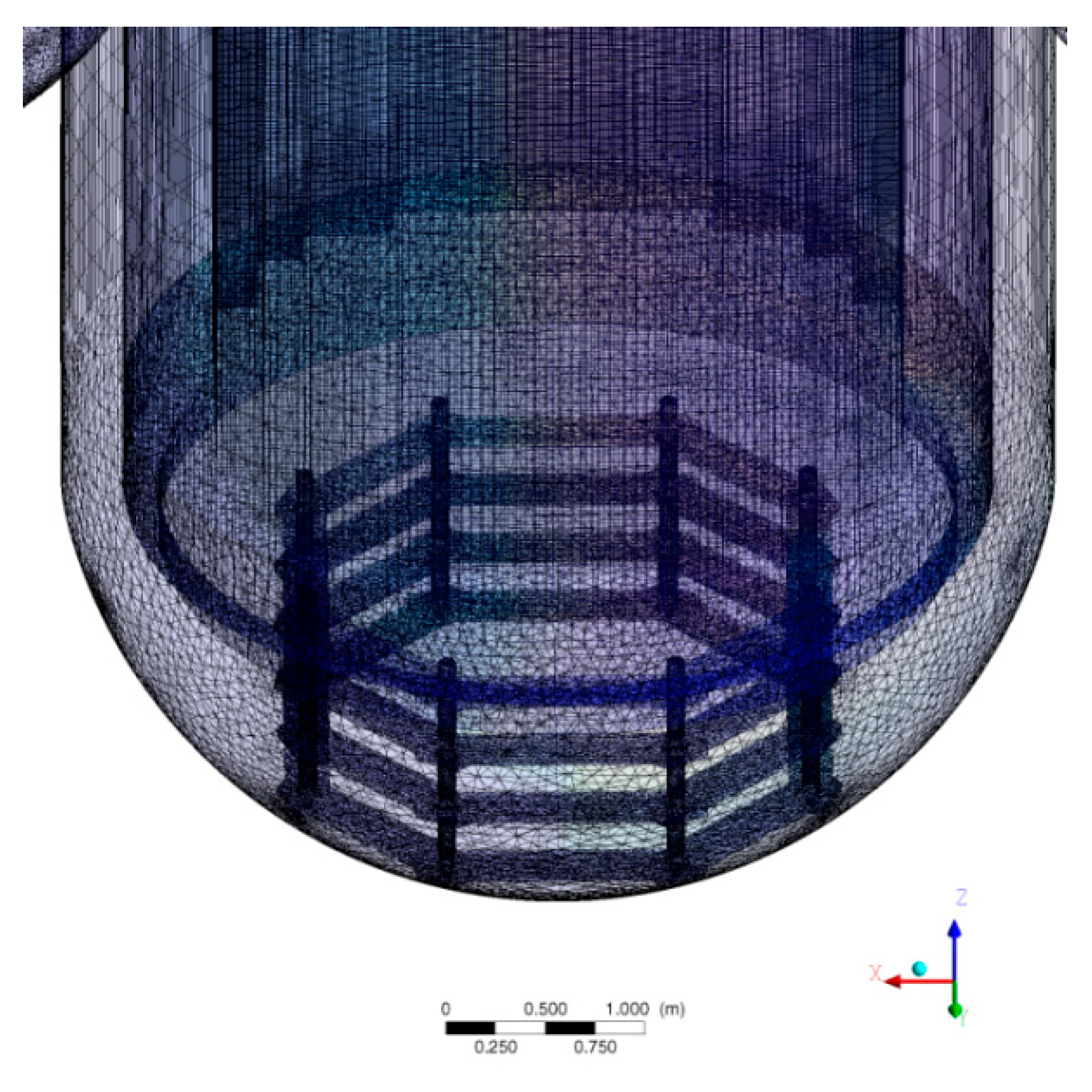
2. Geometry of the CFD Model

The geometry of the CFD model includes the entire RPV with all the relevant details. These include the RPV inlet and outlet nozzles, the hot leg and cold leg parts of the main coolant lines, the downcomer, the lower RPV plenum with internals, the lower core support structure (LCSS), the FAs with the spacer grids and the FA head (Figure 1), the upper core support structure (UCSS) and the installations in the upper RPV plenum.

In Figure 3, the primary circuit of a PWR is shown schematically. The model geometry is outlined in red. Figure 4 shows a top view of the model geometry with the four cold and four hot legs. In Figure 5, the CFD domain of the Pre-Konvoi plant is marked in yellow. Based on the detailed design, the CFD grid model (Figure 6) was created. The complete grid comprises 19.4 million elements, with 13,137,993 tetrahedral elements, 245,024 wedges, 32,318 pyramids and 6,071,267 hexahedral elements. The grid was created using the grid generation program ICEM CFD. The wall area has been greatly refined. Figure 7 shows the core as a simplified porous medium with the spacer planes and the FA head or FA foot. A section through the inlet nozzle plane (z = 0 m) is given in Figure 8.

Figure 9 provides the computational grid. While in the downcomer hexahedral cells dominate, the lower plenum is dominated by tetrahedral cells.

The lower plenum internal (Schemel), which is typical for Pre-Konvoi systems, is shown in Figure 10. This design is intended to equalize the flow in the lower plenum and must be resolved in detail in the modeling in order to correctly capture the flow distribution at the core inlet.

3. Technological Boundary Conditions

The calculations were carried out for normal operating conditions, i.e., for full load operation. The mass flow rate through the core and the resulting pressure losses over the core and over the entire RPV, respectively, were set according to the information obtained from the vendor.

Furthermore, a typical end-of-cycle (EOC) power distribution was assumed in the core. For this purpose, the nodal power distribution was implemented into the CFD model as obtained from a stationary full-core calculation with the neutron kinetics code DYN3D for a generic Pre-Konvoi core loading pattern [2].

In summary, the following technological assumptions were made:

–

Typical EOC power distribution in the core (calculation with DYN3D for a generic Pre-Konvoi core loading pattern, off-line coupling with CFD);

–

Mass flow rate per loop 4910.5 (kg/s);

–

Temperature at the RPV inlet: 293.8 °C;

–

RPV internal pressure: 157 bar (Reactor Inlet).

4. Physical and Numerical Model Properties

The used CFD code ANSYS CFX [3] is a finite-volume CFD program system of state-of-the-art technology for solving the Navier–Stokes equations. The postprocessor enables the extensive qualitative and quantitative analysis of the calculation results. ANSYS CFX-18 relies on unstructured, hybrid computing grids in which tetrahedral, hexahedral, prism and pyramid elements can be combined in any order. Due to the flexible grid generation an optimum representation of complex geometries is possible.

As quality assurance measure grid studies were performed according to the best practice guidelines [4] for CFD applications in nuclear engineering.

The CFD simulations were based on the following assumptions:

–

Adiabatic walls with standard logarithmic wall function;

–

Pressure boundary condition at the hot main coolant pipe legs;

–

Incompressible coolant;

–

Transient CFD calculation with initially quiescent coolant;

–

Second order spatial and temporal discretization scheme;

–

Turbulence model: stress blended eddy simulation (SBES)

In order to reflect the assumed turbulence, the calculations were performed with a hybrid turbulence model. This method combines the advantages of Reynolds Averaged Navier-Stokes equations (RANS) and Large Eddy Simulations (LES), which reduces the modelling part of the RANS and automatically integrates with the grid resolution. As a result, the RANS part near the wall is very high, whereas in the free stream, the vortices are resolved by means of LES.

The SBES turbulence model belongs to the hybrid RANS–LES turbulence model family [5]. SBES allows combining different RANS and LES models with a blending feature to automatically switch between them.

This turbulence model was successfully used to model density-driven flows in ROCOM. The ROCOM mixing test facility provided a unique experimental basis for the validation of CFD tools for the description of turbulent flows [6,7]. Benchmark tests [8] were used to test the turbulence models under different flow conditions to study the influence of reactor geometry, and to analyze the choice of constraints, discretization scheme, time step size, and grid size.

5. Porous Body Modeling of the Core

The core is represented as a heterogeneous anisotropic porous body. This means that the head losses are different for axial (streamwise) and transverse flow. The SG zones have been taken into account in such a way that in these areas no transverse flow is possible. Moreover, the axial head losses are different for SG zones, FA foot, FA head, and the open FA regions between the SGs. The head losses along the axial flow direction, as usually applied in thermal hydraulic system code calculations, are provided in

Table 1. Axial pressure losses in the core region.

	∆p (bar)
FA foot	0.1319
Sum over SG zones:	0.7109
Sum over open FA area:	0.4225
FA head	0.1052
Total:	1.37
LCSS	0.007
UCSS	0.0744

. The axial drag coefficients for the CFD calculations are matched to these pressure drops.

The following sink terms are inserted in the momentum equation:

S_M,_x′ = −μ U_x′/K^S_perm − K^S_loss ρ |U| U_x′/2

(1)

S_M,_y’ = −μ U_y′/K^T_perm − K^T_loss ρ |U| U_y′/2

(2)

S_M,_z´ = −μ U_z′/K^T_perm − K^T_loss ρ |U| U_z′/2

(3)

The permeabilities K^S_perm and the resistance coefficients K^S_loss for streamwise (S) flow are defined as follows:

K^S_perm = U_x′ μ Δx /Δ p [m²]

(4)

K^s_loss = 2 Δp/[ρ |U| U_x′ Δx] [m⁻¹]

(5)

The resistance coefficients for transverse (T) flow direction are set according to the streamwise coefficient multiplier option offered by ANSYS CFX [3]:

K^T_loss = 10 K^s_loss (for SG area, LCSS, UCSS)

(6)

K^T_loss = 2 K^s_loss (for open FA area)

(7)

For the SG area, the LCSS and the UCSS, the multiplier was set to 10 in order to widely block the transverse flow in these areas.

The velocities U_X′, U_Y′, U_Z′ are superficial velocities. In order to convert them into real flow velocities, they need to be divided by the respective porosity (about 0.4 in the vertical and about 0.25 in the horizontal direction). For example, the calculated streamwise superficial velocity of 2 m/s corresponds to a flow velocity of approx. 5 m/s in the core. Similarly, the superficial transversal velocity of 0.05 m/s is equivalent to a transverse flow velocity of 0.2 m/s.

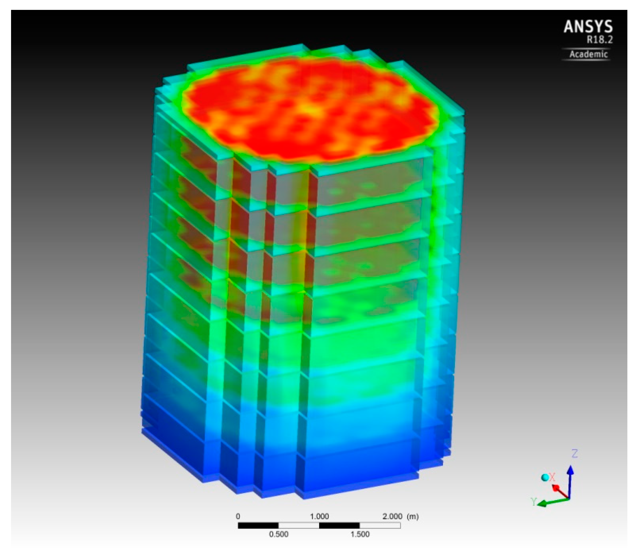
6. Power Distribution within the Core

The power distribution in the reactor core was calculated with the help of a stationary core calculation using the neutron kinetics code DYN3D [9]. DYN3D is a nodal 3D reactor dynamics code for stationary and time-dependent core analyses of light water reactors. The DYN3D burn-up module was used to perform a burn-up calculation for a generic KONVOI equilibrium core loading [10] until the end of the cycle. This generic core contains 64 mixed oxide (MOX) fuel assemblies. The stationary core calculation for determining the power distribution was carried out under the following boundary conditions:

-

Thermal power: 3950 MW;

-

Boron concentration: 50 ppm;

-

Temperature at the core inlet: 293.8 °C;

-

Core mass flow: 19,642 kg/s.

As it is usual with nodal codes, the radial neutron kinetic resolution is one node per fuel assembly. In the thermal hydraulic and fuel rod module, a mean fuel rod per fuel assembly is modeled. The axial resolution is 16 layers and is identical for the neutron kinetics and thermal hydraulics modules of DYN3D. This includes one reflector node at the core bottom and the top, respectively.

Figure 11 and Figure 12 present a horizontal cross-section of the rod linear power rate in the reactor core and the axial distribution of the rod linear power rate of one fuel assembly.

The power distribution calculated with the above boundary conditions was extracted from DYN3D and mapped to 13 equivalent height layers for use in CFX. As a result, 2509 nodal power densities (values for 193 fuel elements in 13 height layers each) were provided. The volume sources thus extracted from the DYN3D calculation were transferred to CFX and interpolated according to the CFX grid. Finally, the power distribution was re-calibrated to the total thermal output of 3950 MW. The resulting mean core heat-up in both calculations (DYN3D and CFX) was approx. 35 K. Figure 13 and Figure 14 show the distribution of the heat sources in the CFX calculation.

7. Results

Figure 15 and Figure 16 present a streamline view of the flow through one sector of the RPV (cold leg sector 1 CL 1). The flow in the downcomer forms sector patterns as can be seen in these figures. The flow is bounded laterally by the coolant flows from the adjacent sectors. Low velocity recirculation areas are located below the cold leg nozzles and high velocity areas between the cold leg nozzles. Figure 17 and Figure 18 show the temperature distribution in the RPV. The coolant is heated up by nuclear fission (in the CFD model by heat source distribution from DYN3D) while flowing through the core (Figure 18) towards the upper RPV plenum. A temperature stratification emerges in the hot legs (hotter medium at the top, see Figure 17).

Figure 19 shows a 3D vector plot of the velocity field in the lower part of the downcomer and in the lower RPV plenum.

While flowing through the lower RPV plenum and the lower plenum internals (Schemel), it is deflected by 180° before it enters the core. Here are recognizable strong vortices. Figure 20 shows the velocity vector views in the upper part of the core between SG levels 8 and 9 (upper part of figure) and in the FA foot area (bottom part of figure), respectively. Different absolute velocities per FA position can be recognized in the FA foot zone, but have almost disappeared in the upper part of the core.

In order to see what really happens to the transverse flow components, a closer view of the velocity field is necessary. Figure 21 shows the nomenclature (SIEMENS KWU) of the fuel element positions in plane view. Additionally, the positions of the cold (KS) and hot legs are indicated. This scheme was used in the following figures.

Figure 22 shows the absolute velocity at the FA positions in a 3D view in the eighth and ninth spacer grid plane (z = −2 m). There is an equal distribution of the velocity in the individual FA positions. Figure 23 displays the transverse velocity component in this plane. Here, it can be stated that this component rises in the direction of the outlet position. Figure 24 illustrates the transversal velocity u, and Figure 25 the transversal velocity v in the FA positions. While the representation of the u component clearly shows that the velocity increases in the direction of the outlet nozzle and is very low in the symmetry plane (H-line), there is no clear trend in the v component. Figure 26 shows the velocity component w. Figure 27 displays the temperature distribution. This is determined by the heat source distribution of the DYN3D calculation.

In the peripheral zones, the temperature increase is lower as well as in the control rod positions. Figure 28, Figure 29, Figure 30 and Figure 31 show the time-dependent transverse velocity components for different planes in three exposed positions (O10, N13 and E2). Starting with Figure 28 in the FA head, these transverse components are the largest. There are also larger fluctuations recognizable. These components become smaller with increasing distance in the direction of the center of the core (downwards) (Figure 29, the eighth and ninth spacer grid-plane, Figure 30, the seventh and eighth spacer grid-plane and Figure 31, the fifth and sixth spacer grid plane) and the fluctuations become smaller. It can also be concluded from the Figure 28, Figure 29, Figure 30 and Figure 31 that transversal velocities are getting larger towards the core outlet depending on the positions of the hot legs (see Figure 21). Closer to the hot legs, the flow is already directed towards it and therefore the transversal velocity components are getting larger.

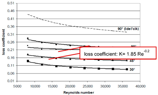
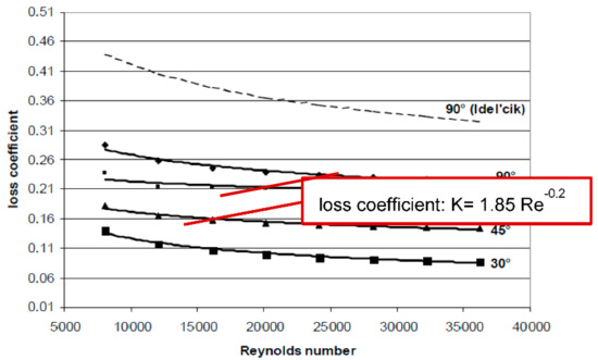
8. Securing the Results with the Wanninger Model Approach [11]

The results of our approach were compared with an approach from the literature [11].

The physical and numerical model properties according to [11] are shown below. As in our approach, the source and sink terms were used in the momentum equation in the CFD code.

The sink terms in the momentum equation are:

S_M,_x′ = −μ U_x′/K^S_perm − K^S_loss ρ |U| U_x′ /2→S^S_perm = −μ U_x′/K^S_perm

(8)

S_M,_y′ = −μ U_y′/K^T_perm − K^T_loss ρ |U| U_y′ /2→S^T_perm = −μ U_y′/K^T_perm

(9)

S_M,_z′ = −μ U_z′/K^T_perm − K^T_loss ρ |U| U_z′ /2→bzw. = −μ U_z′/K^T_perm

(10)

The approach in the flow direction is as follows:

S^S_perm = 0 [m²]

For K^s_loss Wanninger uses the McAdams correlation. However, this provides too small pressure losses. This is why it was chosen for this value:

K^s_loss = 2 Δp/[ρ |U| U_x´ Δ x] [m⁻¹]

(11)

as in our approach. The approach in the transverse direction is determined as follows:

K^T_loss = 1.85 Re^−0.2/p_FR(δ/(δ 1))² (Figure 32)

(12)

with:

p_FR: Fuel rod pitch, δ: Pitch-to-diameter ratio: ${\mathrm{p}}_{\mathrm{FR}}/{\mathrm{d}}_{\mathrm{FR}}$.

The Reynolds number is determined according:

Re = v d_FR/σ

(13)

with d_FR the rod diameter, v the gap velocity, and σ the kinematic viscosity.

Figure 32 shows the loss coefficient as a function of the Reynolds number according to Peybernes. The results of the physical and numerical model properties according to [11] are:

K^T_loss (rods between spacer) = 272 [m⁻¹].

This corresponds to a factor of 68 over our approach (multiplier approach). Our option for more restricted areas is K^T_loss × 2:

K^T_loss (spacer level, OKG, UKG) = 544 [m⁻¹].

The negation of the permeability term in the momentum sink in [11] may lead to an underestimation of the pressure loss at the core: Δp_total (core): 0.78 bar.

A comparison of results is shown in Figure 33, Figure 34, Figure 35 and Figure 36. Figure 33 shows the absolute velocities of the two approaches in the FA foot over the core diameter. As the resistance coefficients in the transversal area are larger according to [11], these influences can already be seen in Figure 34 in the FA foot.

Figure 35 and Figure 36 show a comparison of vector representations in plan view for both model approaches. The figures show in the first and second spacer grid level some small differences.

9. Conclusions

The aim of the study was the detection of possible vortices between the eighth and ninth spacer grid plane of a Pre-Konvoi core, which could lead to temperature cycling. The results of the CFD calculation do not show large dominant vortices in the upper core region. The core acts as a rectifier and dampens large-scale vortices. The analyses included several spacer grid levels in the core and showed that in some areas of the core cross-section, an upward increasingly directed transversal flow to the outlet nozzle occurs. In other areas of the core cross-section, on the other hand, there is nearly any cross-flow.

However, the following limitations of the model apply: in the model, all fuel elements are treated as identical and cross flows due to different axial pressure losses for different FA types cannot be displayed. The complex structure of the FAs (e.g., flow vanes in spacer grids) could also influence the formation of large-scale vortices. This effect could only be resolved with a very high number of grid elements (several billions). This is currently not possible from a computational point of view. In addition, the possible influence of two-phase flows was not considered.

References

1. Prasser, H.-M.; Kliem, S. Coolant mixing experiments in the upper plenum of the ROCOM test facility. Nucl. Eng. Des. 2014, 276, 30–42. [Google Scholar] [CrossRef]
2. Kliem, S.; Gommlich, A.; Grahn, A.; Rohde, U.; Schuetze, J.; Frank, T.; Gomez, A.; Sanchez, V. Development of multi-physics code systems based on the reactor dynamics code DYN3D. Kerntechnik 2011, 76, 160–165. [Google Scholar] [CrossRef]
3. ANSYS CFX Solver Manual; CFX-18; ANSYS: Canonsburg, PA, USA, 2018.
4. Mahaffy, J.; Chung, B.; Song, C.; Dubois, F.; Graffard, E.; Ducros, F.; Heitsch, M.; Scheuerer, M.; Henriksson, M.; Komen, E.; et al. Best Practice Guidelines for the Use of CFD in Nuclear Reactor Safety Applications-Revision; NEA/CSNI/R(2014)11; Organisation for Economic Co-Operation and Development: Paris, France, 2015. [Google Scholar]
5. Menter, F. Stress-Blended Eddy Simulation (SBES)—A New Paradigm in Hybrid RANS-LES Modeling. In Proceedings of the Sixth HRLM Symposium, Strasbourg University, Strasbourg, France, 26–28 September 2016; Available online: https://hrlm6.sciencesconf.org/118745/document (accessed on 21 September 2020).
6. Cartland Glover, G.; Höhne, T.; Kliem, S.; Rohde, U.; Weiss, F.-P.; Prasser, H.-M. Hydrodynamic phenomena in the downcomer during flow rate transients in the primary circuit of a PWR. Nucl. Eng. Des. 2007, 237, 732–748. [Google Scholar] [CrossRef]
7. Höhne, T.; Kliem, S.; Bieder, U. IAEA CRP benchmark of ROCOM PTS test case for the use of CFD in reactor design using the CFD Codes ANSYS CFX and TrioCFD. Nucl. Eng. Des. 2018, 333, 161–180. [Google Scholar] [CrossRef] [Green Version]
8. Huang, M.; Höhne, T. Numerical simulation of multicomponent flows with the presence of density gradients for the upgrading of advanced turbulence models. Nucl. Eng. Des. 2019, 344, 28–37. [Google Scholar] [CrossRef]
9. Rohde, U.; Kliem, S.; Grundmann, U.; Baier, S.; Bilodid, Y.; Duerigen, S.; Fridman, E.; Gommlich, A.; Grahn, A.; Holt, L.; et al. The reactor dynamics code DYN3D—models, validation and applications. Prog. Nucl. Energy 2016, 89, 170–190. [Google Scholar] [CrossRef]
10. Kliem, S.; Rohde, U.; Weiss, F.-P. Core response of a PWR to a slug of under-borated water. Nucl. Eng. Des. 2004, 230, 121–132. [Google Scholar] [CrossRef]
11. Wanninger, A.; Seidl, M.; Macián-Juan, R. Mechanical analysis of the bow deformation of a row of fuel assemblies in a PWR core. Nuclear Eng. Technol. 2018, 50, 297–305. [Google Scholar] [CrossRef]
Figure 1. Fuel assembly (FA) model (Framatome, shortened).
Fluids 05 00161 g001
Figure 2. Area between eighth and ninth spacer grids.
Fluids 05 00161 g002
Figure 3. Primary circuit of a pressurized water reactors (PWRs) model geometry (red).
Fluids 05 00161 g003
Figure 4. Top view of the model geometry.
Fluids 05 00161 g004
Figure 5. Primary circuit Pre-Konvoi PWR, CFD domain (yellow).
Fluids 05 00161 g005
Figure 6. Grid model (cut).
Fluids 05 00161 g006
Figure 7. Core with FA head, FA foot and spacer grids.
Fluids 05 00161 g007
Figure 8. Inlet nozzle plane cut reactor pressure vessel (RPV).
Fluids 05 00161 g008
Figure 9. Grid lower plenum with lower plenum internals.
Fluids 05 00161 g009
Figure 10. Lower plenum internal (Schemel).
Fluids 05 00161 g010
Figure 11. Linear power rate per rod.
Fluids 05 00161 g011
Figure 12. Linear power rate per rod over the height.
Fluids 05 00161 g012
Figure 13. Heat sources in the core, CFX.
Fluids 05 00161 g013
Figure 14. Heat source distribution at a height level between 8th and 9th SG.
Fluids 05 00161 g014
Figure 15. Streamline representation of the velocity field in a sector (CL 1), snapshot.
Fluids 05 00161 g015
Figure 16. Streamline representation of velocity distribution in downcomer and upper plenum, snapshot.
Fluids 05 00161 g016
Figure 17. Coolant temperature in the RPV.
Fluids 05 00161 g017
Figure 18. Coolant temperature in the core region.
Fluids 05 00161 g018
Figure 19. Vector plot of the velocity in the lower RPV plenum.
Fluids 05 00161 g019
Figure 20. Flow velocity vectors in the FA foot zone and between the 8th and 9th SG levels.
Fluids 05 00161 g020
Figure 21. FA positions numbering.
Fluids 05 00161 g021
Figure 22. Absolute velocity (m/s): 8th and 9th plane, z = −2 m, snapshot.
Fluids 05 00161 g022
Figure 23. Transversal velocity (m/s): 8th and 9th plane, z = −2 m, snapshot.
Fluids 05 00161 g023
Figure 24. Transversal velocity u (m/s): 8th and 9th plane, z = −2 m, snapshot.
Fluids 05 00161 g024
Figure 25. Transversal velocity v (m/s): 8th and 9th plane, z = −2 m, snapshot.
Fluids 05 00161 g025
Figure 26. Streamwise velocity w (m/s), 8th and 9th plane, z = −2 m, snapshot.
Fluids 05 00161 g026
Figure 27. Temperature (K), 8th and 9th spacer grid plane, z = −2 m, snapshot.
Fluids 05 00161 g027
Figure 28. Time-dependent transversal velocity FA-head, z= −1.5 m, positions O10, N13 und E2.
Fluids 05 00161 g028
Figure 29. Time-dependent transversal velocity 8th and 9th spacer grid plane, z= −2 m, positions O10, N13 und E2.
Fluids 05 00161 g029
Figure 30. Time-dependent transversal velocity 7th and 8th spacer grid plane, z= −2.5 m.
Fluids 05 00161 g030
Figure 31. Time-dependent transversal velocity 5th and 6th spacer grid plane, z= −3.6 m.
Fluids 05 00161 g031
Figure 32. Loss coefficient as a function of the Reynolds number (Wanninger (2018)).
Fluids 05 00161 g032
Figure 33. Absolute velocity (m/s).
Fluids 05 00161 g033
Figure 34. Transversal velocity u (m/s).
Fluids 05 00161 g034
Figure 35. Vector plot first and second spacer grid level, our approach.
Fluids 05 00161 g035
Figure 36. Vector plot first and second spacer grid level, Wanninger approach.
Fluids 05 00161 g036