Numerical Study of the Magnetic Damping Effect on the Sloshing of Liquid Oxygen in a Propellant Tank


Abstract
1. Introduction
2. Numerical Method
2.1. Computational Model
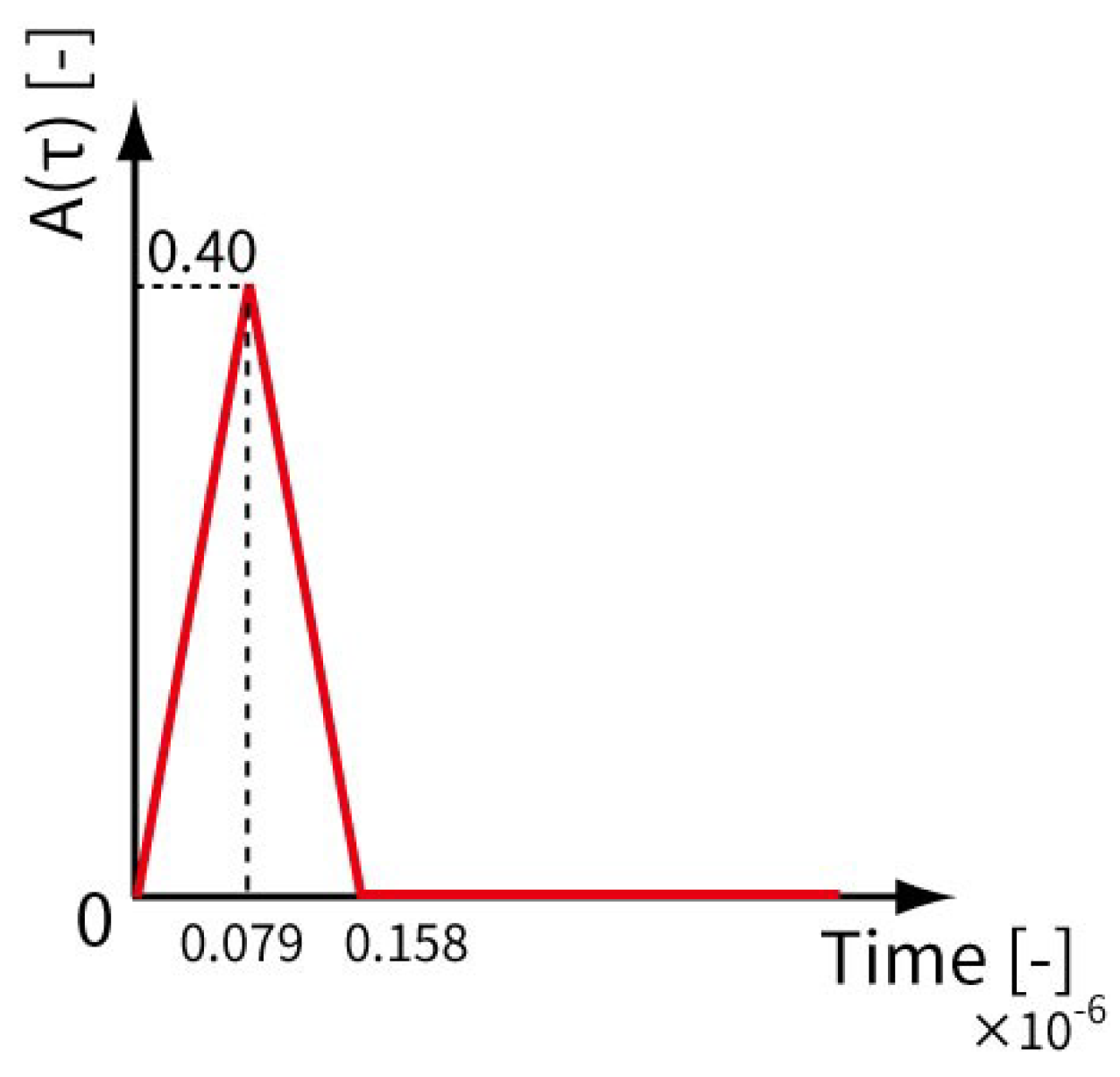
2.2. Initial Condition
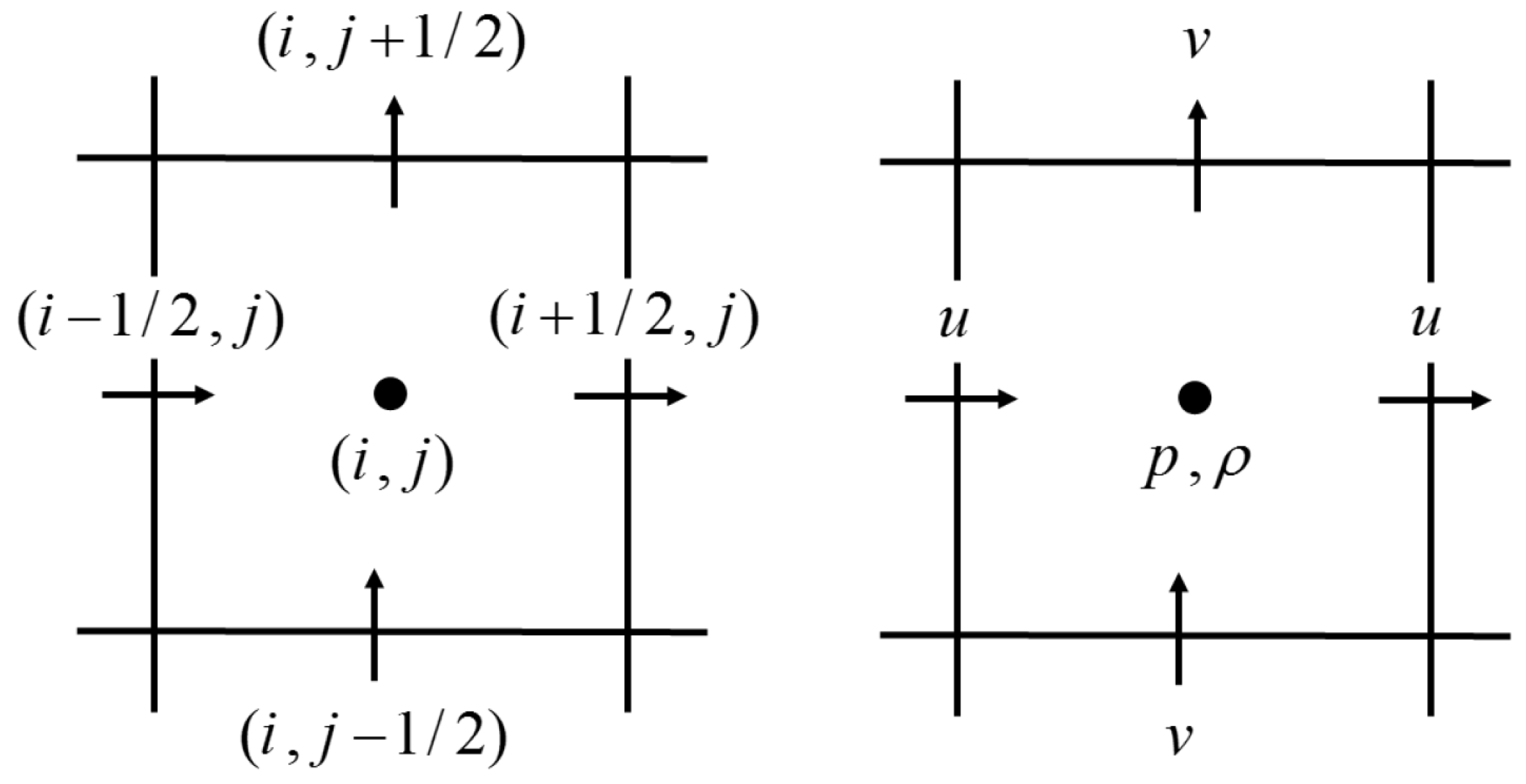
2.3. Computational Grid
2.4. Model of Two-Phase Flow
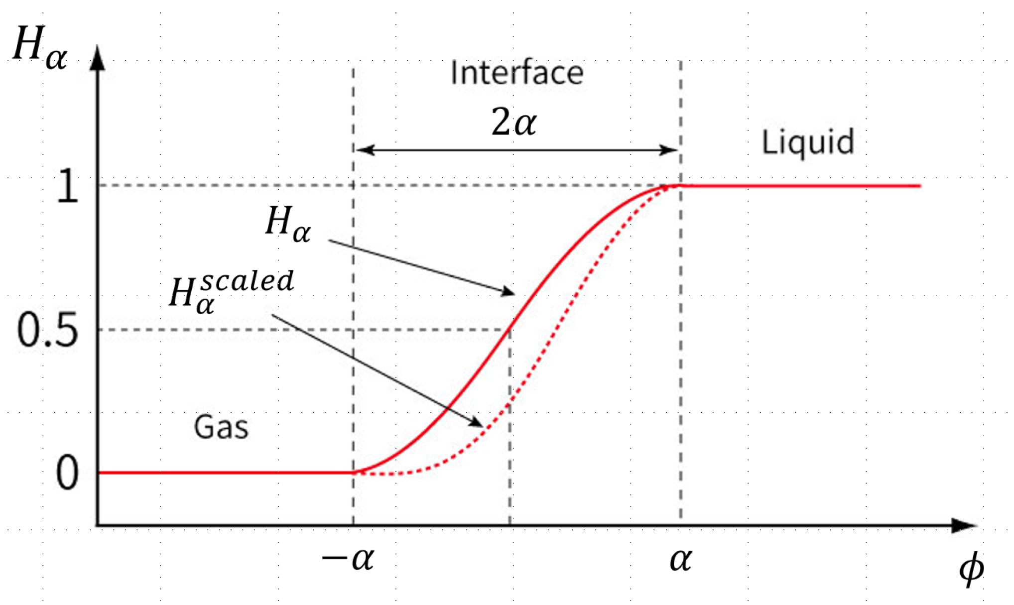
2.5. Method to Capture the Dynamic Surface
2.6. Governing Equation
- Dimensionless variables
- Dimensionless numbers
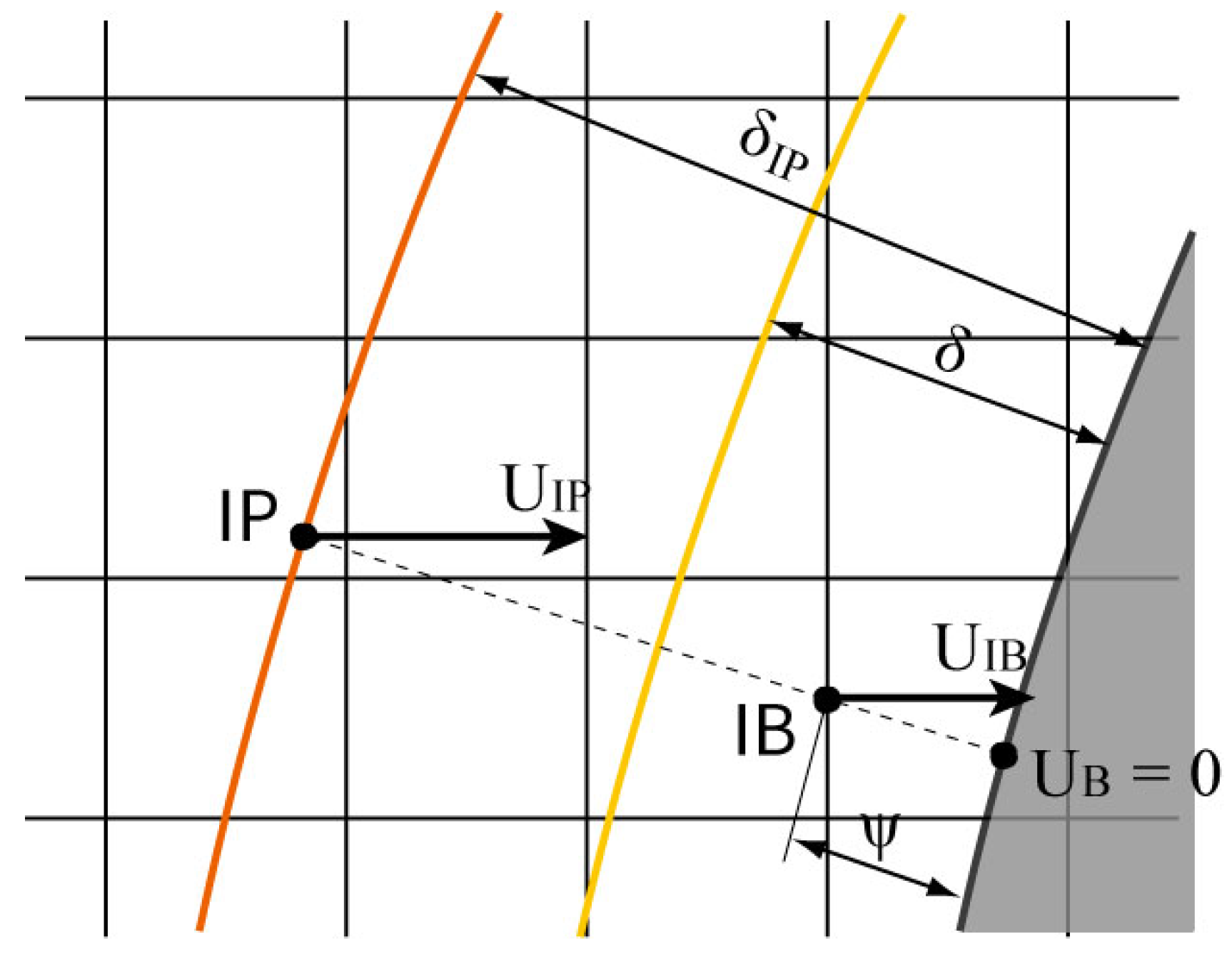
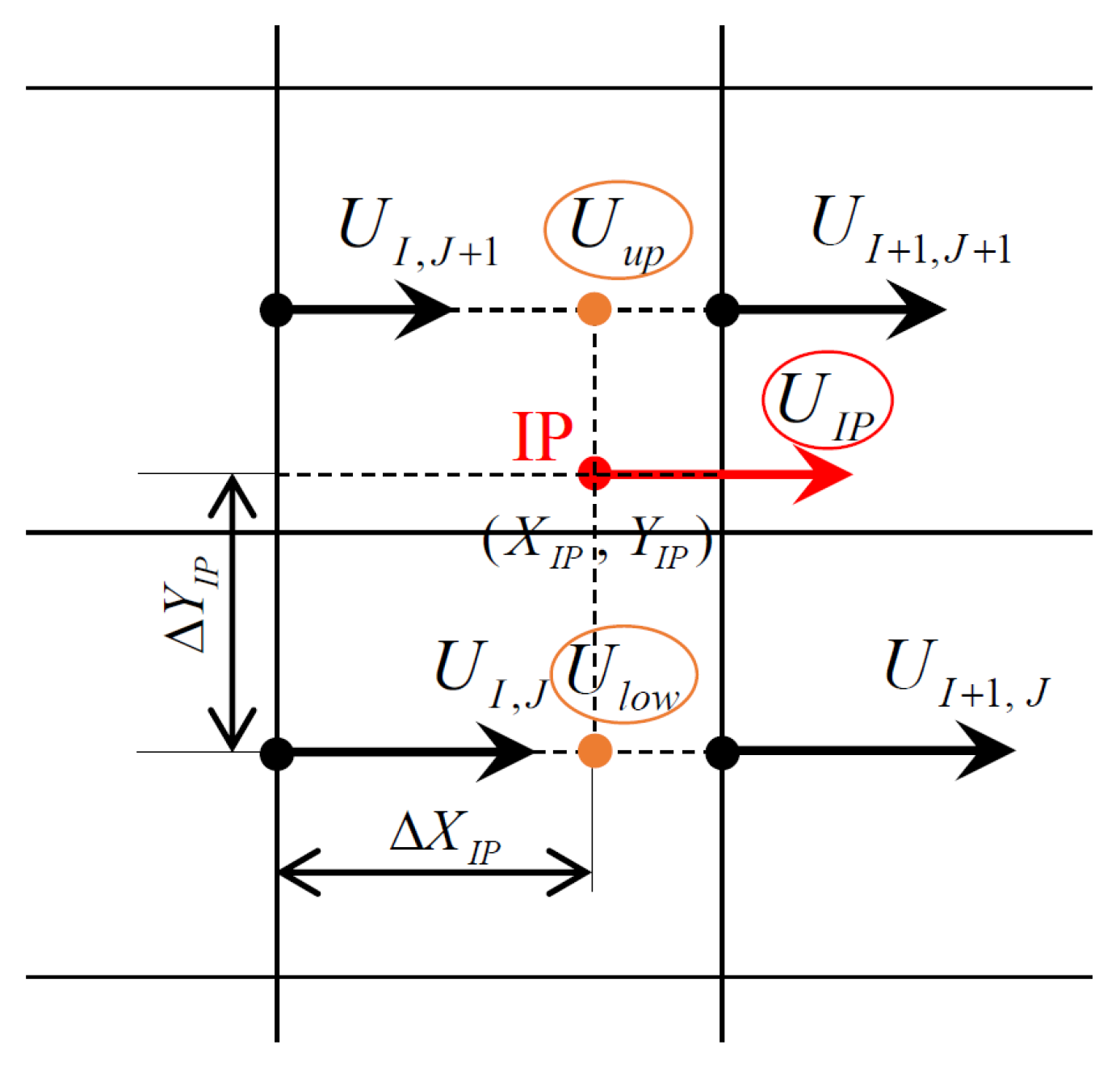
2.7. IB (Immersed Boundary) Method
2.8. Boundary Condition
2.9. Pressure Correction
2.10. Parameters for Computation
3. Validation of the Numerical Method
4. Results and Discussion
5. Conclusions
- When the magnetic flux density at the center of the coil was the same, the sloshing damping effect tended to be higher when the coil surface was closer to the tank than when the coil diameter was equal to the tank.
- When the magnetic flux density at the center of the coil was 1.0 T, the sloshing was dampened to a certain extent, and by setting the magnetic flux density at the center of the coil to 3.0 T, a sufficient sloshing damping effect was obtained. Actually, it is anticipated that even if less than 3.0 T, the damping effect is sufficient by placing the coil closer to the tank. This has the potential to contribute to the damping of the center of gravity movement of spacecrafts and the prevention of mixing of ullage gas into the piping.
- Future tasks include speeding up the computation, improving the IB method, and introducing wettability to an arbitrary shaped wall. Besides, it is necessary to evaluate quantitatively the shift of the center of gravity in the tank and the thermal behavior when the sloshing is dampened by a magnetic field.
Author Contributions
Funding
Conflicts of Interest
Nomenclature
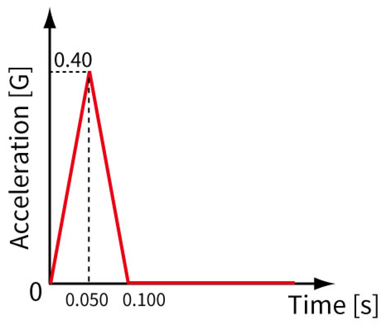
| Acceleration as a function of time | [] | |
| Acceleration as a function of dimensionless time | [-] | |
| Magnetic flux dencity at the center of the coil | [T] | |
| Corrected magnetic flux density vector | [T] | |
| Magnetic flux density vector by Biot–Savart law | [T] | |
| Corrected dimensionless magnetic flux density vector | [-] | |
| Dimensionless magnetic flux density vector by Biot-Savart law | [-] | |
| C | VOF function | [-] |
| D | Dimensionless coil diameter | [-] |
| Unit vector in the direction of excitation force | [-] | |
| Magnetizing force vector | [] | |
| Dimensionless magnetizing force vector | [-] | |
| Surface normal force vector | [] | |
| Dimensionless surface normal force vector | [-] | |
| g | Gravitational acceleration | [] |
| Ga | Galilei number | [-] |
| Density-scaled Heaviside function | [-] | |
| Coil current | [A] | |
| l | Characteristic length (Tank diameter) | [m] |
| L | Dimensionless characteristic length (Tank diameter) | [-] |
| M | Dimensionless number representing the strength of the magnetic field | [-] |
| p | Pressure | [Pa] |
| P | Dimensionless pressure | [-] |
| Position vector of the coil | [m] | |
| Dimensionless position vector of the coil | [-] | |
| t | Time | [s] |
| Velocity vector | [m/s] | |
| Dimensionless velocity vector | [-] | |
| Dimensionless velocity vector on the wall | [-] | |
| Dimensionless velocity vector at IB point | [-] | |
| Dimensionless velocity vector at IP | [-] | |
| X-direction component of | [-] | |
| Y-direction component of | [-] | |
| Position vector in the calculation area | [m] | |
| Dimensionless position vector in the calculation area | [-] | |
| Number of grids in the X, Y, Z direction | [-] | |
| Grid width in the X, Y, Z direction | [-] | |
| Greek letters | ||
| Interface thickness | [m] | |
| Dimensionless interface thickness | [-] | |
| Surface tension | [N/m] | |
| Laplace number | [-] | |
| Distance to IP | [-] | |
| Local mean curvature at interface | [1/m] | |
| Dimensionless interface curvature | [-] | |
| Viscosity of gas phase | [] | |
| Viscosity of liquid phase | [] | |
| Viscosity ratio | [-] | |
| Dimensionless viscosity | [-] | |
| Magnetic permeability in vacuum | [H/m] | |
| Circle ratio | [-] | |
| Density of gas phase | [] | |
| Density of liquid phase | [] | |
| Density ratio | [-] | |
| Dimensionless density | [-] | |
| Dimensionless time | [-] | |
| Dimensionless calculation time | [-] | |
| Level set function | [m] | |
| Scalar potential | [-] | |
| Dimensionless level set function | [-] | |
| Mass magnetic susceptibility of gas phase | [] | |
| Mass magnetic susceptibility of liquid phase | [] | |
| Mass magnetic susceptibility ratio | [-] | |
| Dimensionless magnetic susceptibility | [-] | |
| Distance function from wall surface | [-] |
References
- Himeno, T. Propellant Management in Liquid Rockets and Space Vehicles. J. Jpn. Soc. Multiph. Flow 2013, 27, 385–392. [Google Scholar] [CrossRef][Green Version]
- Himeno, T. Liquid Motion in the Propellant Tanks of Space Vehicles. J. Jpn. Soc. Fluid Mech. Nagare 2013, 32, 239–244. [Google Scholar]
- Maemura, T.; Gotou, T.; Akiyama, K.; Nimura, K.; Watanabe, A. New H-IIA Launce Vehicle Technology and Maiden Flight Results. Mitsubishi Heavy Ind. Tech. Rev. 2002, 39, 43–50. [Google Scholar]
- Gen, M.; Ogasawara, K.; Kitayama, O.; Ochiai, T. Conceptual Study of Space Environmental Experiment Platform using H-IIA 2nd Stage. Int. Symp. Space Technol. Sci. 2008. Unpublished work. [Google Scholar]
- Kitayama, O.; Tokunaga, T.; Igarashi, I.; Okita, K.; Fujita, M. Cryogenic Propellant Management of H-IIA Upper Stage. Int. Symp. Space Technol. Sci. 2006. Unpublished work. [Google Scholar]
- Abramson, H.N. (Ed.) The Dynamic Behavior of Liquids in Moving Containers. In NASA SP-106; National Technical Information Service: Springfield, VA, USA, 1966. [Google Scholar]
- Demirel, E.; Aral, M.M. Liquid Sloshing Damping in an Accelerated Tank Using a Novel Slot-Baffle Design. Water 2018, 10, 1565. [Google Scholar] [CrossRef]
- Jamalabadi, M.Y.A.; Ho-Huu, V.; Nguyen, T.K. Optimal Design of Circular Baffles on Sloshing in a Rectangular Tank Horizontally Coupled by Structure. Water 2018, 10, 1504. [Google Scholar] [CrossRef]
- Zheng, X.; You, Y.; Ma, Q.; Khayyer, A.; Shao, S. A Comparative Study on Violent Sloshing with Complex Baffles Using the ISPH Method. Appl. Sci. 2018, 8, 904. [Google Scholar] [CrossRef]
- Ohashi, A. Effects of Baffle Plate on Cryogenic Fluid Sloshing and Pressure Fluctuation. Bachelor’s Thesis, The University of Tokyo, Tokyo, Japan, 2015. [Google Scholar]
- Furuichi, Y.; Ohashi, A.; Kameyama, S.; Haba, D.; Sakuma, Y.; Uzawa, S.; Himeno, T.; Watanabe, T. Effects of Thermal Stratification Thickness on Cryogenic Fluid Sloshing and Pressure Fluctuation. In Proceedings of the 57th Aeronautics and Astronautics Propulsion Conference, Okinawa, Japan, 9 March 2017. [Google Scholar]
- Brackbill, J.U.; Kothe, D.B.; Zemach, C. A Continuum Method for Modeling Surface Tension. J. Comput. Phys. 1992, 100, 335–354. [Google Scholar] [CrossRef]
- Yokoi, K. A density-scaled continuum surface force model within a balanced force formulation. J. Comput. Phys. 2014, 278, 221–228. [Google Scholar] [CrossRef]
- Yokoi, K. A practice numerical framework for free surface flows based on CLSVOF method, multi moment meth od and density scaled CSF model: Numerical simulation of droplet splashing. J. Comput. Phys. 2013, 232, 252–271. [Google Scholar] [CrossRef]
- Yokoi, K. Efficient implementation of THINC scheme: A simple and practical smoothed VOF algorithm. J. Comput. Phys. 2007, 226, 1985–2002. [Google Scholar] [CrossRef]
- Sakuraba, M.; Hirosaki, S.; Kashiyama, K. Development of Accurate Interface-Capturing method for Free Surface Flow Analysis based on CIVA/VOF method. J. Appl. Mech. 2003, 6, 215–222. [Google Scholar] [CrossRef]
- Bednarz, T.; Tagawa, T.; Kaneda, M.; Ozoe, H.; Szmyd, J.S. Magnetic and gravitational convection of air with a coil inclined around the X axis. Numer. Heat Transf. Part A Appl. 2004, 46, 99–113. [Google Scholar] [CrossRef]
- Tagawa, T.; Ozoe, H. Effect of Prandtl number and computational schemes on the oscillatory natural convection in an enclosure. Numer. Heat Transf. Part A Appl. 1996, 30, 271–282. [Google Scholar] [CrossRef]
- Neu, J.T.; Good, R.J. Equilibrium behavior of fluids in containers at zero gravity. AIAA J. 1963, 1, 814–819. [Google Scholar] [CrossRef]
- Utsumi, M. Low-Gravity Sloshing in an Axisymmetrical Container Excited in the Axial Direction. J. Appl. Mech. 2000, 67, 344–354. [Google Scholar] [CrossRef]
- National Institute of Standards and Technology Material Measurement Laboratory. Thermophysical Properties of Fluid Systems. Available online: http://webbook.nist.gov/chemistry/fluid/ (accessed on 5 December 2019).
- National Astronomical Observatory of Japan. Magnetic susceptibility of paramagnetic and diamagnetic substance. In Chronological Scientific Tables Premium; Maruzen Publishing: Tokyo, Japan, 2019; Available online: http://www.rikanenpyo.jp/member/?module=Member&action=Login (accessed on 21 April 2020).
- Tagawa, T.; Ozoe, H. Effect of external magnetic fields on various free-surface flows. Prog. Comput. Fluid Dyn. 2008, 8, 461–468. [Google Scholar] [CrossRef]


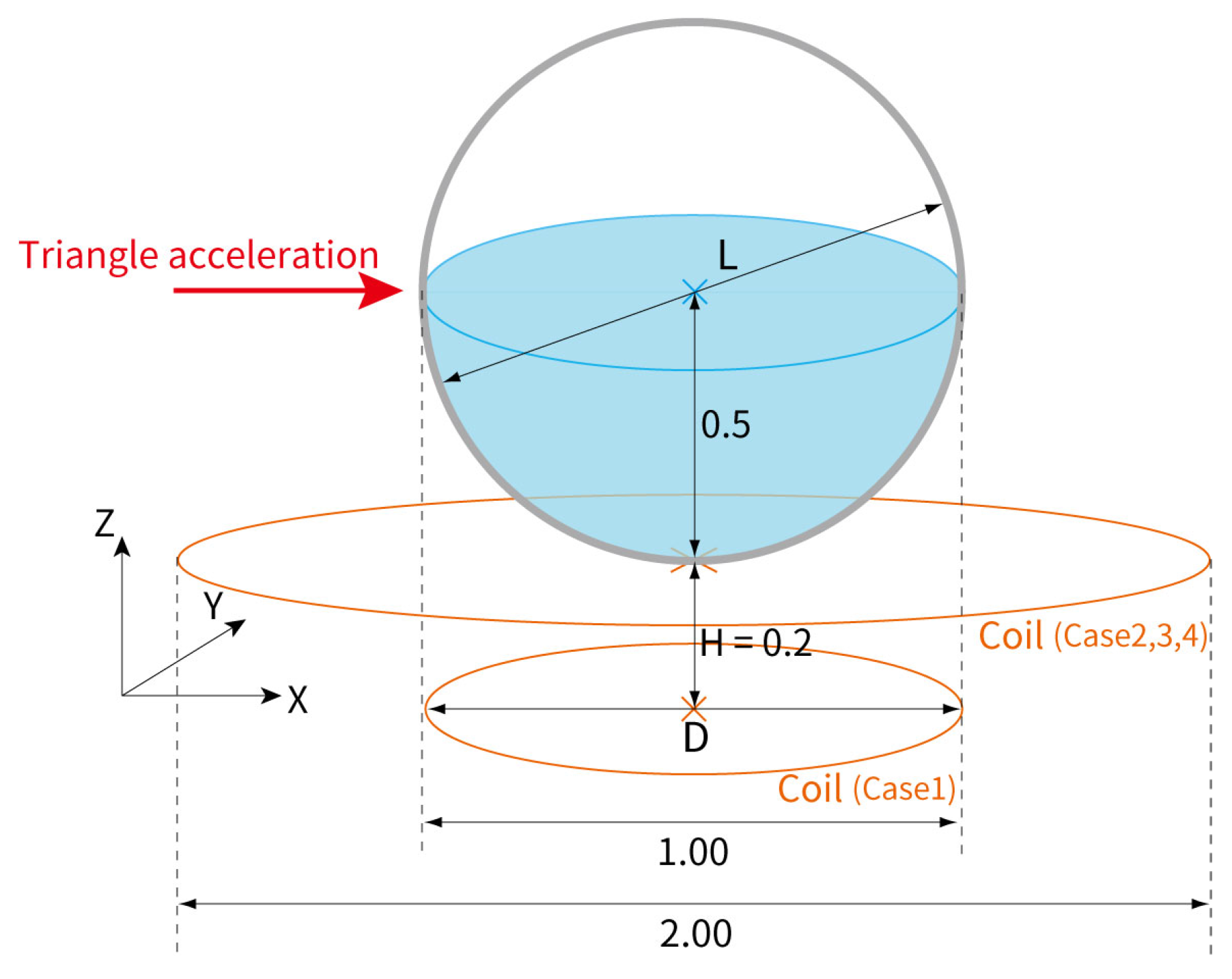
| Case No. of Computational Conditions | Case 0 | Case 1 | Case 2 | Case 3 | Case 4 |
|---|---|---|---|---|---|
| Dimensionless height of the coils (H) [-] | −0.2 | 0.0 | 0.0 | 0.0 | |
| Ratio of coil diameter to characteristic length (D/L) [-] | No coil | 1.0 | 2.0 | 2.0 | 2.0 |
| Magnetic flux density at the center of coils () [T] | 1.0 | 0.1 | 1.0 | 3.0 |
| Parameter | Symbol | Value | Unit |
|---|---|---|---|
| Characteristic length (diameter of spherical tank) | l | 1.00 | [m] |
| Density of gaseous oxygen | 4.4509 | [] | |
| Density of LOX | 1141.4 | [] | |
| Viscosity of gaseous oxygen | [] | ||
| Viscosity of LOX | [] | ||
| Mass magnetic susceptibility of gaseous oxygen | [] | ||
| Mass magnetic susceptibility of LOX | [] | ||
| gravitational acceleration | g | 9.80665 | [] |
| Surface tension | [N/m] |
| Parameter | Symbol | Value (Dimensionless) |
|---|---|---|
| Number of grids | 80, 80, 80 | |
| Number of grids per tank diameter | (None) | 64 |
| Computation time | ||
| Time step | ||
| Density ratio | 256 | |
| Viscosity ratio | 28.0 | |
| Magnetic susceptibility ratio | 2.23 | |
| Galilei number | Ga | |
| Laplace number | ||
| Dimensionless number about magnetic field | M | Case1: Case 2: Case 3: Case 4: |
| Parameter | Symbol | Value (Dimensionless) |
|---|---|---|
| Number of grids | 64, 64, 64 | |
| Number of grids per characteristic length | (None) | 32 |
| Computation time | ||
| Time step | ||
| Density ratio | 100 | |
| Viscosity ratio | 10.0 | |
| Magnetic susceptibility ratio | 0.0 | |
| Galilei number | Ga | 0.0 |
| Laplace number | ||
| Dimensionless number about magnetic force | M | 0.0 |
© 2020 by the authors. Licensee MDPI, Basel, Switzerland. This article is an open access article distributed under the terms and conditions of the Creative Commons Attribution (CC BY) license (http://creativecommons.org/licenses/by/4.0/).
Share and Cite
Furuichi, Y.; Tagawa, T. Numerical Study of the Magnetic Damping Effect on the Sloshing of Liquid Oxygen in a Propellant Tank. Fluids 2020, 5, 88. https://doi.org/10.3390/fluids5020088
Furuichi Y, Tagawa T. Numerical Study of the Magnetic Damping Effect on the Sloshing of Liquid Oxygen in a Propellant Tank. Fluids. 2020; 5(2):88. https://doi.org/10.3390/fluids5020088
Chicago/Turabian StyleFuruichi, Yutaro, and Toshio Tagawa. 2020. "Numerical Study of the Magnetic Damping Effect on the Sloshing of Liquid Oxygen in a Propellant Tank" Fluids 5, no. 2: 88. https://doi.org/10.3390/fluids5020088
APA StyleFuruichi, Y., & Tagawa, T. (2020). Numerical Study of the Magnetic Damping Effect on the Sloshing of Liquid Oxygen in a Propellant Tank. Fluids, 5(2), 88. https://doi.org/10.3390/fluids5020088