Flow in Fractured Porous Media Modeled in Closed-Form: Augmentation of Prior Solution and Side-Stepping Inconvenient Branch Cut Locations

Abstract

Carefully chosen complex variable formulations can solve flow in fractured porous media. Such a calculus approach is attractive, because the gridless method allows for fast, high-resolution model results. Previously developed complex potentials to describe flow in porous media with discrete heterogeneities such as natural fractures can be modified to expand the accuracy of the solution range. The prior solution became increasingly inaccurate for flows with fractures oriented at larger angles with respect to the far-field flow. The modified solution, presented here, based on complex analysis methods (CAM), removes the limitation of the earlier solution. Benefits of the CAM model are (1) infinite resolution, and (2) speed of use, as no gridding is required. Being gridless and meshless, the CAM model is computationally faster than integration methods based on solutions across discrete volumes. However, branch cut effects may occur in impractical locations due to mathematical singularities. This paper demonstrates how the augmented formulation corrects physically unfeasible refraction of streamlines across high-permeability bands (natural fractures) oriented at high angles with respect to a far-field flow. The current solution is an important repair. An application shows how a drained rock volume in hydraulically fractured hydrocarbon wells will be affected by the presence of natural fractures.

1. Introduction

Fast and accurate solutions for flow in fractured porous media are sought after in the petroleum industry, which increasingly extracts oil and gas from hydraulically and naturally fractured shale formations. Practical applications for flow models of fractured porous media are ubiquitous and not limited to the petroleum industry. For example, medical applications involving flow across fractured bone structures, and magmatic melts moving from the Earth’s mantle to the crust via pore space and fractures also are governed by equations for flow in fractured porous media. Of particular interest to the current study is the modeling of the flow of hydrocarbon fluids in fractured reservoirs, for which our models can provide detailed solutions. However, the formulation provided here may also be applied to subsurface flow studies for geothermal energy extraction from naturally fractured rocks.

Modeling flow in fractured porous media with discrete fractures using explicit numerical methods is computationally intensive and requires excessive meshing and gridding adjustments near fracture intersections [1,2,3,4]. An alternative model approach, advocated here, uses a gridless and meshless analytical modeling technique based on complex analysis methods (CAM), and has been stepwise developed in two key, earlier papers. The first paper [5] presented a solution using areal doublets, which is accurate for flow through fractures aligned with a far-field flow and can account for an unlimited (but finite) number of fractures and any permeability contrast between the fractures and matrix. The second paper [6] resolved branch cut choices arising in solutions of the real part (potential function) of the complex potential for areal doublets, which is relevant when plotting the pressure fields involving flow near natural fractures.

We revisit the superposition process used to derive the expressions for an areal doublet and an areal dipole, developed in the two prior studies [5,6] to model flow in fractured porous media. In these prior studies, instantaneous stream function solutions were used to visualize streamlines in porous media with randomly oriented fractures [5]. The potential function, with appropriate scaling, was used to plot the pressure field [6]. The velocity field can also be solved in every location and, combined with an Eulerian particle tracking method, enables the construction of fluid particle paths for time-dependent flows and allows for the insertion of time-of-flight (TOF) contours to show the flow advance at specific time increments after the onset of flow [7].

This study augments the prior solutions [5,6] by removing certain limitations when the method is applied to fractures oriented at high angles to the far-field flow. Although the code used in previous studies is accurate for flow near fractures at low angles to the ambient (far-field) flow direction, the earlier solution does not adequately account for flow through natural fractures at a high angle to the far-field flow direction. The augmentation proposed in the present study provides a comprehensive solution, valid for any orientation of the natural fractures and does not require (manual) adjustments for high-angle fractures, as was the case in the prior code.

This article proceeds as follows. Section 2 first explains the functionality of the existing closed-form algorithms to describe flow in fractured porous media. Section 3 presents the augmented solution, which can account for flow near the fractures at any angle with the far-field flow. Section 4 presents a field case application of the augmented algorithms. A discussion follows in Section 5, and conclusions are given in Section 6.

2. Complex Potential Solutions

In this section, we revisit some fundamental closed-form solutions required to ultimately adjust complex potentials used to describe flow through discrete fracture systems. Redirection of streamlines can be effectuated when an existing flow, described by a set of single-valued complex potentials is superposed by a complex potential that represents the desired disturbance. For example, Figure 1a shows an undisturbed flow between a direct line drive with streamlines connecting a series of injectors and producer wells. The basic flow pattern will be altered when a rectangular domain of high permeability is placed in the flow path between the injector and producers; the streamlines converge (with a faster time-of-flight) toward the producer wells (Figure 1b). The opposite occurs (i.e., a slower time-of-flight) when the rectangular domain instead has a lower permeability than the surrounding matrix, which will result in streamline divergence (Figure 1c). Both the flow convergence and divergence (in Figure 1b,c) were modeled by superposing a series of line doublets [7].

Section 2 moves through three systematic steps that highlight how the line doublets and related line dipoles are transformed into areal doublets and line dipoles that are suitable for modeling flow through discrete natural fractures in a reservoir. First, Section 2.1 explains the difference between the line doublet and a line dipole, which are two end members of a continuous series of line doublet/line dipole intermediates. Next, Section 2.2 reviews the prior complex potential used for closed-form flow models of fractured porous media and gives a comprehensive complex potential which can describe both the areal doublet and areal dipole. Section 2.3 highlights the limitations to the practical use of the derived solution due to branch cut effects. The results of Section 2 are necessary for an amended solution given in Section 3 that avoids the branch cut effects.

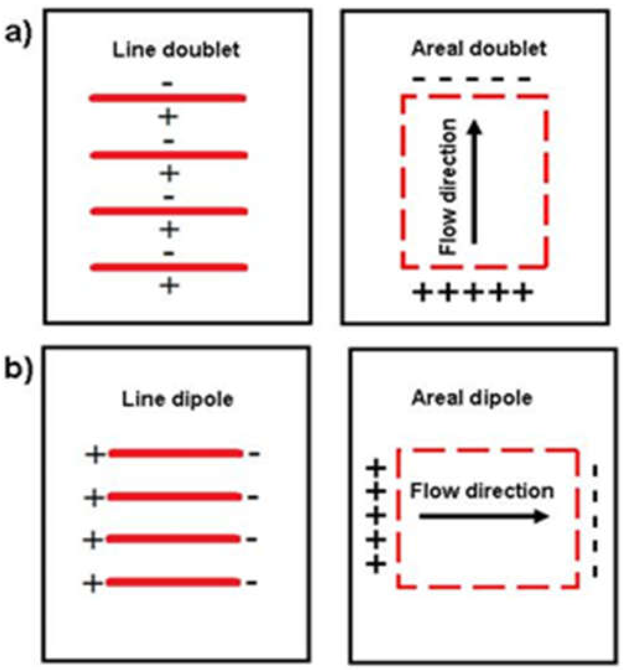
2.1. Line Doublets and Line Dipoles

The distinction between doublets and dipoles was originally proposed by Strack [8], and was required for constructing line arrays called, respectively, line doublets and line dipoles. The line doublet is composed of a linear array of superposed singularity doublets (Figure 2a). The polarity of each singularity doublet [defined by its source (+) and sink (−) sides] remains perpendicular to the line array at all times (Figure 2a). Similarly, the line dipole is a linear array of superposed singularity dipoles (Figure 2b). In the line dipole, the source and sink sides of the singularity are rotated 90° clockwise, and thus the polarity of each dipole remains aligned with the line array at all times (Figure 2b).

The complex potential for a line doublet and a line dipole are invariant [6], which means these potentials represent two physically distinct flows. The comprehensive solution presented below shows that the invariant nature of the respective complex potentials does not preclude the formulation of a concise complex potential that covers a broader spectrum of physical flows, including the line doublet and line dipole as end-members. The comprehensive solution is given by the following complex potential (Ω) [5]:

$${\mathsf{\Omega }}_1(z,t)=\frac{m(t)e^{i\theta }\cdot e^{i\beta }}{2\pi nH}\frac{[Log(z-z_a)-Log(z-z_b)]}{(z_a-z_b)}$$

(1)

with strength m(t) [m⁴ s⁻¹], unit depth H [m], and porosity n. A practical way to rewrite Equation (1) is to introduce $z_a=z_c-0.5W{e}^{i\beta }$ and $z_b=z_c+0.5W{e}^{i\beta }$[9], where W, z_c and $\beta$ are the width, center coordinates and tilt angle of the line doublet/dipole element. The need to have two complex coordinates (z_a and z_b) is removed, and instead the mid-point (z_c) between the two ends of the region occupied by the flow element is given by specifying a width W. The polarity of the singularity doublet/dipole can be controlled by $\theta$. For $\theta =90°$, we obtain the line doublet solution given in Weijermars and Van Harmelen [9]. However, when $\beta =0$°, the angle $\theta$ of the doublet singularities in the line element does not need to be 90°. For $\theta =0$° we have the line dipole solution. Intermediate flow types occur for $90°<\theta <0°$ (see below).

There are two separate methods to obtain the streamlines for flows described by the complex potential of Equation (1). The first method separates the real and imaginary parts of the complex potential to obtain, respectively, the potential function and the stream function. The solutions for the stream function and the potential function can then be obtained (for any steady-state flow moment at time t) as an integral solution with standard software packages (like MATLAB, Python, Mathematica or others), as follows:

$$\psi (z)=\Im [\mathsf{\Omega }(z)]$$

(2a)

$$\varphi (z)=\Re [\mathsf{\Omega }(z)]$$

(2b)

Figure 3a–d are solutions for $\psi$ and $\varphi$ using Equations (1) and (2a,b), with the input data of

Table 1. Inputs data for line doublet/dipole element in Figure 3.

Quantity	Value	Units	Symbol
Matrix Porosity	0.1		n
Center of the line element	0	m	zc
Length	10	m	L
Tilt angle	0	°	β
Strength	0.01	m4 s−1	m(t)
Height	1	m	H
Polarity	(a) 90°, (b) 45°, (c) 10°, (d) 0°	°	θ

, and various angles for doublet polarity given by $\theta$. Figure 3a–d confirm that the complex potential of Equation (1) gives a continuous solution series for physically viable flows ranging from the line doublet (Figure 3a) to the line dipole (Figure 3d), via intermediate flow types (Figure 3b,c). The stream function solutions are in the left column. The corresponding potential function solutions appear in the right column.

The second method to plot the streamlines for the flow of Equation (1) is to trace individual particles with an Eulerian particle tracking method. The particle tracking for any particular flow is made possible by first deriving the velocity field from the complex potential specific to the flow of concern, using:

$$V(z,t)=\frac{\overline{d\mathsf{\Omega }(z,t)}}{dt}=v_x+i{v}_y;V(z,t)=\frac{d\mathsf{\Omega }(z,t)}{dt}=v_x-i{v}_y$$

(3a)

Application of the derivative of Equation (3a) to the complex potential of Equation (1), using $z=x+iy=\left|z\right|(\cos \theta +i\sin \theta )=r(\cos \theta +i\sin \theta )=r{e}^{i\theta }$, gives:

$$V(z)=\frac{m\cdot e^{i\theta }\cdot e^{i\beta }}{2\pi nH}\frac{1}{(z-z_b)(z-z_a)}=\frac{m\cdot e^{i\theta }\cdot e^{i\beta }}{2\pi nH}\frac{1}{(z-(z_c+0.5W\cdot e^{i\beta }))(z-(z_c-0.5W\cdot e^{i\beta }))}$$

(3b)

Equation (3b) is the generalized line doublet/dipole equation, which can be used to generate the velocity field for any line doublet/dipole analytical element with an angle of β to the real axis measured in an anti-clockwise direction. Additionally, θ can be used to change the angle of the polarity of the singularities, which collectively makes the line element. As before, for a special case when θ = 90°, e^iθ = i, this equation becomes identical to Equation (C9) for the line doublet in Weijermars and van Harmelen [9] and Equation (B2) in van Harmelen and Weijermars [5]. Note that the complex conjugate $\overline{z}=r{e}^{-i\theta }$, and Euler’s formula $e^{i\theta }=\cos \theta +i\sin \theta$ gives for $\theta =0$° $e^{i\theta }=1$, and for $\theta$= 90° it follows that $e^{i\theta }=i$.

Equation (3b) gives ($v_x,v_y$) for fluid particles in each location of the flow field. The particle tracking method uses a time-step, $\Delta t$, and initial particle position $z_0$ at time $t_0=0$ to track the streamlines followed by the particles. The position $z_1(t_1)$ of the tracer at time $t_1=t_0+\Delta t$ is:

$$z_1(t_1)\approx z_0(t_0)+v(z_0(t_0))\cdot \Delta t$$

(4a)

The position $z_j(t_j)$ of the tracer particles at any other future time $t_j$ is:

$$z_j(t_j)\approx z_{j-1}(t_{j-1})+v(z_{j-1}(t_{j-1}))\cdot \Delta t$$

(4b)

Figure 4a–d show the streamlines for the complex potential of Equation (1), based on the particle tracking method of Equations (3b) and (4a,b) using selected angles $\theta$ and tilt angle of the line element $\beta$ = 0°. Streamline solutions of Equations (3b) using the Eulerian particle tracking method of Equations (4a,b) offer the advantage that so-called time-of-flight contours (TOFCs) can be constructed [7]. Additionally, the flow is integrated over time and the particle paths represent the true flow path of time-dependent flows. The TOFCs show the advancement of an infinite number of tracers for periodic (constant) time-steps.

Comparison of Figure 3a–d and Figure 4a–d reveals that the two methods provide the same streamline solutions. The first approach (stream function approach; Figure 3a–d) gives additional information on the fluid fluxes (stream function values relative to the origin). The alternative particle tracking method (Figure 4a–d) gives additional information on the time-of-flight, which is useful for studies of hydrocarbon drainage and reservoir depletion [7], studies of geothermal reservoirs that require monitoring of the advancement of injected fluids [9], and for studies of subsurface flow including the tracking of pollution plumes.

2.2. Areal Doublets and Areal Dipoles

Section 2.1 has shown that a comprehensive complex potential exists for a suite of flows ranging from the line doublet (Figure 3a) to the line dipole (Figure 3d), via intermediate flow types (with arbitrary oblique orientations of the singularity doublets/dipoles in the respective line array (Figure 3b,c).

A prior study has integrated an infinite number of line doublets to formulate a complex potential for an areal doublet (Figure 5). The flow field of an areal doublet can be interpreted as an infinite number of doublet singularities with poles aligned with the direction of flow as schematically shown in Figure 5a. The complex potential ${\mathsf{\Omega }}_1(z,t)$ for the areal doublet, scaled by a flow strength $\upsilon (t)$ [m⁴s⁻¹] is [5]:

$${\mathsf{\Omega }}_2(z,t)=\frac{\upsilon (t)}{2\pi nHLW}\left[\Re [A-B+C-D]+i\cdot \Im [A-B+C-D]\right]$$

(5)

with dimensions of the areal doublet given by reservoir depth, H, doublet length, L, and aperture (or width), W, with porosity, n. The dummy terms A − D in the real and imaginary parts $\Re [A-B+C-D]$ and $\Im [A-B+C-D]$, for an areal doublet with corner points located at z_a1, z_a2, z_b1, and z_b2, and tilt angle $\gamma$ with the real axis (Figure 6), are as follows:

$$A=-i\cdot e^{-i\gamma }[(z+z_{a2})(\log (-e^{-i\gamma }(z-z_{a2}))]$$

(6a)

$$B=-i\cdot e^{-i\gamma }[(z+z_{a1})(\log (-e^{-i\gamma }(z-z_{a1}))]$$

(6b)

$$C=-i\cdot e^{-i\gamma }[(z+z_{b1})(\log (-e^{-i\gamma }(z-z_{b1}))]$$

(6c)

$$D=-i\cdot e^{-i\gamma }[(z+z_{b2})(\log (-e^{-i\gamma }(z-z_{b2}))]$$

(6d)

With corner point co-ordinates given by:

$$\begin{array}{l}{z}_{a1}=z_c-{\mathrm{e}}^{i\gamma }\cdot (0.5L+0.5W\cdot e^{i\beta })\\ z_{a2}=z_c-{\mathrm{e}}^{i\gamma }\cdot (0.5L-0.5W\cdot e^{i\beta })\\ z_{b1}=z_c-{\mathrm{e}}^{i\gamma }\cdot (-0.5L+0.5W\cdot e^{i\beta })\\ z_{b2}=z_c-{\mathrm{e}}^{i\gamma }\cdot (-0.5L-0.5W\cdot e^{i\beta })\end{array}$$

(7)

A generic, comprehensive complex potential can be formulated for both areal doublets/areal dipoles (Figure 5a,b), and areal flow elements with singularity doublets/dipoles oriented oblique to the boundaries of the areal flow element. In analogy to Equation (1), the prior solution of an areal doublet [5,6] given here in Equation (5), can be modified into a general complex potential for areal doublets/dipoles (Figure 5a), as follows:

$$\begin{array}{ll}{\mathsf{\Omega }}_3(z,t)& =\frac{\upsilon (t)\cdot e^{i(\theta +\beta -\gamma )}}{2\pi nHL}\\ & \left[\frac{\left[(z-z_{a2})\log (-e^{-i\gamma }(z-z_{a2})\right.)-(z-z_{a1})\log (-e^{-i\gamma }(z-z_{a1}))+(z-z_{b1})\log (-e^{-i\gamma }(z-z_{b1}))\left.-(z-z_{b2})\log (-e^{-i\gamma }(z-z_{b2}))\right]}{W\cdot e^{i\beta }}\right]\end{array}$$

(8)

With the corner-point coordinates again given by Equation (7). The solution of Equation (8) differs from the prior solution of Equation (5) in that the doublet/dipole polarity is separately parameterized, by not necessarily letting $\theta =\beta$. The velocity potential corresponding to Equation (8) is given by:

$$\begin{array}{ll}V(z,t)& =\frac{\upsilon (t)\cdot e^{i(\theta +\beta -\gamma )}}{2\pi nHL}\\ & \left[\frac{\left[\log (-e^{-i\gamma }(z-z_{a2}))-\log (-e^{-i\gamma }(z-z_{a1})\right.)\left.+\log (-e^{-i\gamma }(z-z_{b1}))-\log (-e^{-i\gamma }(z-z_{b2}))\right]}{W\cdot e^{i\beta }}\right]\end{array}$$

(9)

This is the general equation that allows for setting the angle of all the analytical elements (point dipole/doublet (θ) to line dipole/doublet (β) to areal dipole/doublet (γ)). In Equations (6) and (7), we have the imaginary i in the equation and we have e^iβ in the denominator, which will cancel each other out for all the cases, and is kept only to maintain analogy with the previous Equations (1) and (5).

The streamlines can again be obtained from Equation (8) applying the stream function and the potential function solutions of Equations (2a,b). First, only $\theta$ is varied for an areal doublet/dipole that has $\gamma =0°$ and $\beta =90°$ (Figure 7a–f), for angles $\theta$ similar to those used for the line doublet/dipole in Figure 3a–d. The solution of Equation (9) correctly shows the morphing transitions of a pure areal doublet (Figure 5a) to a pure areal dipole (Figure 5b).

2.3. Branch Cut Effects

Equation (8) correctly solves the streamlines for a generic areal doublet/dipole element and can be used to represent the streamline deflections occurring near high permeability fractures in fractured porous media. The solutions of Figure 8 show the progressive rotation of a fracture element and the stationary far-field flow (superposed on the doublet-dipole flow) by selecting $\theta$ such that $\theta +\gamma =180°$, for a variety of angles $\gamma$. The composite complex potential, ${\mathsf{\Omega }}_{Comp}(z,t)$, including the complex potential for the uniform far-field flow, ${\mathsf{\Omega }}_4(z,t)=e^{i\theta }{u}_{\infty }(t)z$ (with $u_{\infty }(t)$ already being the effective velocity, accounting for porosity) is:

$${\mathsf{\Omega }}_{Comp}(z,t)={\mathsf{\Omega }}_3(z,t)+{\mathsf{\Omega }}_4(z,t)$$

(10)

The streamline solutions given in Figure 7 and Figure 8 are perturbed by the branch cuts emanating from the singularities, which cause “apparent” jumps in the stream function values from positive to negative, and vice versa. For the areal doublet (Figure 5a), the branch cut seems not to occur, but these are present as a row of singularities in the high and low streamline values. The corresponding potential function solutions also exhibit branch cuts jumps, which we discussed in considerable detail in a prior study [6].

The issue we now face is to move the branch cuts for the general solution to a place where they would not render the use of the Equations (8) and (9) impractical. For the pure areal doublet (Figure 5a), we have earlier succeeded to find a practical branch cut placement solution [6]. However, as pointed out by Holzbecher [10], available procedures for removing branch cut effects from analytical solutions remain limited.

In spite of numerous efforts in our present research program to move the branch cuts from the general solutions of Equations (8) and (9) to a practical location, we did not succeed, which meant that we could not apply Equations (8) and (9) in practical situations that required continuous Eulerian particle tracking. The next section discusses an alternative, augmented solution for areal doublet representation of flow deflections by discrete natural fractures of arbitrary orientation, which solves the prior limitation.

3. Augmented Solution

A new flow element used to model flow in fractured porous media was generated by the integration of line doublets [5]. The derived flow element was initially termed a natural fracture element [5], but later renamed as an areal doublet [6]. The reason for the re-examination of the earlier approach is that the existing formulation is accurate for fractures aligned with a far-field flow, and works well for fractures oriented moderately obliquely with respect to the far-field flow, but becomes increasingly inaccurate when the fractures are perpendicular to or at a large angle to the far-field flow.

3.1. Shortcomings of the Prior Solution

Figure 9 illustrates the problem arising when the simple area doublet formulation of Equation (5) is used to progressively increase the angle of the natural fracture (represented by a narrow areal doublet) relative to a steady far-field flow. A long and narrow fracture aligned with the far-field flow direction can be modeled accurately with an areal doublet (Figure 9a). However, for the larger incidence angles, the flow solution is no longer accurate. Figure 9f shows the solution for a fracture at a large angle to the far-field. The areal doublet would require reorientation of the polarities in the fracture to align with the far-field flow. If we try to implement such polarity changes using Equation (9), the branch cut effects do not allow continuous particle tracking across the fracture region.

To develop an augmented solution, while avoiding the branch cut effects, we first discuss the two end-members, areal doublet and areal dipoles, in some detail (Section 3.2 and Section 3.3) paying specific attention to the orientation of corner point co-ordinates given in Equation (7). Ultimately, the branch cut issues that rendered Equation (9) impractical for use in real world problems were sidestepped by superposing the two end-members of the areal doublet/dipole family of solutions.

3.2. Areal Doublet Solution

The stream function solutions of the areal doublet of Equation (5) with the integral method are given in Figure 10a,b for the two extreme orientations of the natural fracture prototype (vertical and horizontal, as in Figure 9a,f), with a superposed far-field flow. Figure 10c,d show the areal doublet flow without the superposed far-field flow. The solutions given in Figure 10 are possible with Equation (5) while avoiding undue branch cuts by changing the corner point co-ordinates given in Equation (7), according to the respective L/W pairs of the fracture slots (as indicated in the sketches next to the respective solutions). When applied to Eulerian particle tracking, Equation (5) gives continuous solutions, as illustrated in the example of Figure 9. However, for the larger inclinations of the natural fracture element with respect to the far-field flow direction (e.g., Figure 9e,f) the solutions for the flow paths become unrealistic. The initial repair of the natural fracture algorithm occurred via the steps in Section 2.2. However, the proposed algorithms of Equation (8) resulted in multiple branch cuts, which make the continuous Eulerian tracking of particle movement impossible to use. We investigated numerous avenues to move branch cuts to locations where they would not cause multivalued functions along the particle paths, using our experience of a prior study [6]. All efforts failed, except for one approach via the steps explained in Section 3.3 and Section 3.4.

3.3. Areal Dipole Solution

The alternative model for the long fracture aligned with the far-field flow is given by the complex potential for the areal dipole [6]:

$${\mathsf{\Omega }}_5(z,t)=\frac{i\upsilon (t)}{2\pi nHLW}\left[\Re [A-B+C-D]+i\cdot \Im [A-B+C-D]\right]$$

(11)

Equations (5) and (11) differ in that their real and imaginary axes are switched, which is achieved by multiplying the complex potential of Equation (5) with the imaginary number i. The dummy terms A − D remain unchanged and are given by Equations (6a)–(6d). Figure 11a–d are solutions for the areal dipole for the same orientations as in Figure 10a–d, with and without a superposed far-field flow. The solutions given in Figure 11 are possible with Equation (11) while avoiding undue branch cuts by changing the corner point co-ordinates given in Equation (7), according to the respective L/W pairs of the fracture slots (as indicated in the sketches next to the respective solutions). Although the solutions of Figure 10 and Figure 11 appear the same, the important difference lies in the coordinate transformation, due to which the orientations of the examples shown in each set of Figures are swapped 90°. This is a simple but essential step to correctly model the flow across natural fracture elements at a high angle to the far-field flow (see Section 3.4). The branch-cut effects that impeded continuous particle tracking across the natural fracture element with the solution of Equations (8) and (9) do not occur with the solution enabled by the superposition of Equations (5) and (11), given in Section 3.4.

3.4. Superpositions

Changing the corner point co-ordinates according to the respective L/W pairs of the fracture slots as applied in Figure 10 and Figure 11 will avoid the occurrence of branch cuts in impractical places, but is not very user-friendly when superposing multiple fracture elements in practical applications. Thus, the velocity fields for two areal doublets are superposed with the velocity field of the far field flow, such that the two end angles (0° and 90°) result in the correct particle-path solutions based on the conceptual model of Figure 12.

For the intermediate cases, where the tilt angle is between the two end angles, the contribution of each element (0° and 90°) is proportioned by using the sine function. The vertical solution has a more dominant effect when the natural fractures oriented at an angle lower than 45° (more parallel to the fluid flow) and vice versa. The superposed complex potential (with the augmented solution in the second term on the right-hand side) is:

$$\mathsf{\Omega }(z)={\mathsf{\Omega }}_f(z)+{\displaystyle \sum _{n=1}^2{(-1)}^{n+1}}\sin {\gamma }_n·{\mathsf{\Omega }}_n(z)$$

(12)

${\mathsf{\Omega }}_f(z)$ is complex potential for the far-field flow given by:

$${\mathsf{\Omega }}_f(z)=u_{\infty }(t)z$$

(13)

${\mathsf{\Omega }}_n(z)$ is the complex potential for the areal doublet/dipole element given by:

$$\begin{array}{l}{\mathsf{\Omega }}_n(z)=\frac{-\upsilon (t)}{2\pi hn\cdot L_n\cdot W_n}·e^{-i(\gamma -{\theta }_n)}\cdot [(z+z_{a2n})(\log (-e^{-i\gamma }(z-z_{a2n}))-(z+z_{a1n})(\log (-e^{-i\gamma }(z-z_{a1n}))\\ +(z+z_{b1n})(\log (-e^{-i\gamma }(z-z_{b1n}))-(z+z_{b2n})(\log (-e^{-i\gamma }(z-z_{b2n}))]\end{array}$$

(14)

The vertices $z_{a1n}$, $z_{a2n}$, $z_{b1n}$, and $z_{b2n}$ are the vertices for the areal doublet/dipole element given by:

$$\begin{array}{l}{z}_{a1n}=z_c-{\mathrm{e}}^{i\gamma }\cdot (0.5L_n+0.5W_n\cdot e^{i\beta })\\ z_{a2n}=z_c-{\mathrm{e}}^{i\gamma }\cdot (0.5L_n-0.5W_n\cdot e^{i\beta })\\ z_{b1n}=z_c-{\mathrm{e}}^{i\gamma }\cdot (-0.5L_n+0.5W_n\cdot e^{i\beta })\\ z_{b2n}=z_c-{\mathrm{e}}^{i\gamma }\cdot (-0.5L_n-0.5W_n\cdot e^{i\beta })\end{array}$$

(15)

The transformations and inputs needed to calculate the vertices given in Equation (15) are given below:

$$\begin{array}{l}{\theta }_1=(\pi /2)\\ {\theta }_2=-{\theta }_1\\ {\gamma }_2={\gamma }_1-(\pi /2)\\ L_2=W_1\\ W_2=L_1\end{array}$$

(16)

Figure 13 shows the particle path across a single, highly conductive fracture at different orientations with respect to a far-field flow incoming from below generated by using the velocity potential derived from Equation (12). The length (L₁) and the width (W₁) were assumed to be 10 m and 1 m respectively. The results in Figure 13 show more plausible flow paths compared to the results in Figure 9 for the cases where the fracture is tilted at an angle of more than 45° with respect to the direction of the far-field flow.

4. Application

In this section, the augmented solution for flow across discrete fractures will be applied to a practical situation. Natural fractures may have a significant impact on the performance and flow of hydraulically fractured wells tapping into hydrocarbon reservoirs [11]. The interaction of hydraulic and natural fractures makes forecasting the performance of wells in such reservoirs a major challenge [12,13]. Alternatively, conductive natural fractures may promote pressure communication between the adjoining hydraulic fractures and wells, which increase the well/fracture interference [14]. The nonconductive natural fractures may affect the sweep pattern due to waterflood between the injector and the producer wells [15]. Hence, the estimation of a reservoir’s flow performance and overall production depends on accurate description of the flow diversion due to the presence of natural fractures and natural fracture networks. Section 4.1 provides a brief background on different modeling methods for naturally fractured reservoirs.

Natural fractures distort the drained rock volume (DRV) around hydraulic fractures and may result in pressure communication with fractures of the adjoining stages and wells. The DRV is defined as the reservoir volume that contributes to oil and gas production through the movement of fluid particles to the wellbore after a particular specified production period. Although there is movement of fluid particles throughout the reservoir, only a limited fraction of those particles reaches the wellbore in a reasonable time period, which is shown by the DRV. Unusual refractions of streamlines near the well system occurred in our prior model code (compare Figure 9f and Figure 13f) when natural fractures were oriented at a high angle to the far-field flow direction. We revisit the examples presented in an earlier study (in Section 4.2), where the effect of natural fractures on the DRV was investigated by using the algorithm presented in Equation (5) [16]. In Section 4.3, the DRV is regenerated using the modified solution of Equation (12). Finally, in Section 4.4, we compare results obtained earlier [16] with the results from the modified algorithm presented in this paper. The DRV for the reservoirs where natural fractures are oriented in the direction of flow remains unchanged. However, the DRV for the reservoirs where the natural fractures are oriented at a high angle to the far-field flow direction show a drastic change. A brief validation of the augmented solution is given in Section 4.5.

4.1. Flow in Fractured Reservoirs

Oil and gas reservoirs may contain vast networks of natural fractures, which interact with the hydraulic fractures, and therefore the most accurate flow simulation and production forecasting models must strive to account for the impact of natural fractures, based on their orientation, distribution, connectivity, strength and interaction with the hydraulic fractures [17,18]. Previously, naturally fractured reservoirs were mainly modeled by using dual porosity and modifications of the dual porosity model [19,20]. These models consider natural fractures as a secondary continuum with up-scaled flow properties, but have limited accuracy, and cannot be used to model discrete fracture networks [21]. Another widely used technique uses discrete fracture network (DFN) models [22] and embedded discrete fracture network models (EDFM) [23]. Such discrete models have some benefits over dual porosity models, such as flexibility and give more accurate representations of the fracture network, but they are computationally very demanding and expensive for complex reservoirs with numerous natural fractures. Both the continuum model (dual porosity) and the discrete model (DFN, EDFM) have been thoroughly reviewed in our prior study [16].

Hence, there is a need for new fast and gridless methods (such as the one presented in this study), which allow for efficient modeling of fluid flow in naturally fractured reservoirs. The present study builds forward on the earlier studies where closed-form analytical solutions based on complex analysis methods (CAM) were applied to single-phase flow reservoirs, assuming either hydraulic fractures only [24] or hydraulic fractures intersecting with natural fractures [6]. The natural fracture algorithms have been used in fundamental studies of the equivalent tensor concept [25]. An advantage of CAM models over numerical models is the ability to visualize the drained rock volume (DRV) with infinite resolution.

Unlike discretized numerical simulators, the CAM simulator offers enhanced visual resolution of the DRV around the hydraulic and natural fractures. Flow visualization at high resolution can be especially important to optimize fracture and well spacing in already crowded shale fields with several horizontal wells and hydraulic fractures. The prior studies [24,25] used an algorithm developed earlier [5], which works well when the natural fractures are oriented in the direction of the fluid flow. However, the algorithm needs to be modified when the natural fractures occur at larger angles to the direction of the fluid flow, as illustrated in the following section.

4.2. Field Application: Flow Near Hydraulic Fractures

In this section, we revisit some results of our previous study [16], which presented an extensive collection of results where natural fractures of varying orientations were introduced to a base case (Figure 14), and were simulated using Equation (5).

Figure 14a shows the streamlines (blue color) for a full-scale model of a hydraulically fractured well. The particle paths are generated only for the middle five hydraulic fractures for computational efficiency. However, the flow toward all the hydraulic fractures in the complex plane (119 fractures) is accounted for in the model simulation and were simulated for a period of 30 years. The identical hydraulic fractures, each of which has a fracture half-length of 150 ft (45.7 m) and height of 60 ft (18.3 m), are assumed to have a constant flux of 13.6 ft³/day (0.39 m³/day) per fracture, which is equivalent to the hydraulic fracture (line sink) strength of 8.47 ft²/day (0.79 m²/day). The rainbow colors in Figure 14b show the time of flight contours (TOFC), where each different color represents the DRV expansion for three-year increments from five hydraulic fractures (one stage) in the center of the well.

When natural fractures are present in the reservoir, the DRV shape around the hydraulic fractures will be progressively distorted when natural fractures (oriented oblique—at 45°—to the horizontal well) occur in the proximity of the hydraulic fractures. The permeability contrast between the matrix and the fractures is increasing from the left to the right (

Table 2. Input summary for reservoir and natural fractures simulated in Figure 14 and Figure 15. Modified from [8].

Attributes of Reservoir and Hydraulic Fractures
Reservoir height				60 ft (18.3 m)
Porosity				4.4%
Hydraulic fracture half-length				150 ft (45.7 m)
Residual oil saturation				0.25
Initial Strength (m0)				8.47 ft2/day (0.79 m2/day)
Formation volume factor (B)				1.05 RB/STB
Attributes of Areal Doublets (Natural Fractures)
Figure	Length	Width	Height (ft)	No. of natural fractures	Orientation (with respect to wellbore)	Strength (ft4/day)	Permeability Contrast Ratio
15a	150 ft (45.7 m)	3 ft (0.91 m)	60 ft (18.3 m)	6	45°	6 × 103 ft4/day 51.8 m4/day	7.87
15b	150 ft (45.7 m)	3 ft (0.91 m)	60 ft (18.3 m)	14	45°	6 × 103 ft4/day 51.8 m4/day	7.87
15c	150 ft (45.7 m)	3 ft (0.91 m)	60 ft (18.3 m)	6	10°	60 × 103 ft4/day 518 m4/day	78.68
15d	150 ft (45.7 m)	3 ft (0.91 m)	60 ft (18.3 m)	14	10°	60 × 103 ft4/day 51.8 m4/day	78.68

). Figure 15c,d shows the DRV distortion due to highly conductive natural fractures oriented at a high angle with respect to the far-field flow (10°) to the horizontal well). The natural fracture permeability contrast with the matrix (and corresponding strengths) and other properties for each of the cases are presented in Table 2. The DRV, for each case (Figure 15a–d), is distorted. However, where natural fractures have steep angles with respect to the far-field flow, the resulting sideward deflection of the particle paths appeared physically unrealistic (Figure 15c,d). As shown earlier (in Figure 9), the application of Equation (5) leads to such unrealistic particle paths for steep natural fractures. For higher angles to the far-field flow direction, the results of Figure 15c,d present an improved solution (Section 4.3).

4.3. Augmented Solution for Flow Near Hydraulic Fractures with Natural Fractures

Next, we implement the augmented solution of Equation (12) and rerun the results, aimed at removing any unrealistic particle paths seen in Figure 15. Figure 16a–d shows the DRV generated from the augmented solutions corresponding to the cases shown in Figure 15a–d. Comparison of the DRVs for the first two cases (Figure 15a,b and Figure 16a,b) show minimal effect due to the change in algorithms because the natural fractures are oriented at a moderate angle of 45° to the direction of the particle paths. However, the DRV distortion intensifies for highly conductive natural fractures oriented at a large angle to the far-field flow direction (Figure 15c,d), as can be calculated from the augmented equation (Equation (12)).

4.4. Comparison of Results Augmented and Earlier Solution

The DRV shapes of Figure 15c,d and Figure 16c,d differ significantly. The extreme deflection of particle paths seen in Figure 15c,d does not occur in Figure 16c,d, due to the application of the augmented code based on Equation (12). The extent of the fluid plume drained from the reservoir reaches farther into the reservoir (up to 1000 ft or 305 m, with natural fractures) for all cases (even after the application of the augmented solution), as compared to only 800 ft (244 m) in a reservoir without natural fractures (Figure 14b) or with few natural fractures oriented at moderate angles to the far-field flow (Figure 15a,b and Figure 16a,b).

4.5. Verification

Finally, the augmented solution is verified here in a straightforward experiment, which compares the prior solution of Equation (5) with the augmented solution of Equation (12). Consider a square domain with a higher permeability than the ambient matrix. The flow through the domain can be simulated by superposing an areal doublet of a certain strength on the far-field flow (

Table 3. Natural fracture attributes for fractures oriented at different angles.

Natural Fracture Attributes	Symbol	Value
Natural fracture width (m)	W	5
Natural fracture length (m)	L	5
Natural fracture height (m)	H	1
Natural fracture angle to far-field flow	α	(a) 90° (b) 60° (c) 0°
Porosity	n	0.1
Effective far-field flow rate (m/s)	ux/n	3.12 × 10−8
Effective natural fracture strength (m4/s)	υ/n	2.97 × 10−6

), similar to what is shown in Figure 1b. The left column in Figure 17 gives the prior solution for three angles using Equation (5). The right column gives the flow behavior according to the augmented solution. The left bottom image in Figure 17 shows the problem arising when the prior solution is at a large angle with respect to the far-field flow: fluid appears to be deflected in a horizontal direction, which is physically unrealistic. The problem does not occur for the 90° rotated square [bottom right; using Equation (12)], which shows the same flow behavior as for the topmost right image, henceforth the solution for the large incidence angle may be assumed to be correct.

5. Discussion

The areal doublet is an analytical element formed by superposing an infinite number of line doublets. The mathematical function can be used to model the physical flow of fluids in highly conductive, narrow flow-channels such as natural fractures [5,6]. The areal doublet locally accelerates the flow of fluids due to the enhanced permeability contrast with the matrix and can be superposed with other flow elements such as nearby hydraulic fractures to model the fluid withdrawal patterns (drained rock volume—DRV) in hydraulically fractured hydrocarbon and geothermal reservoirs [8,23]. The work presented here provides a modification of the algorithm for an areal doublet, which corrects the high deviation of streamlines, when the areal doublet is not parallel to the direction of the fluid flow. The original equation (Equation (5)) results in the same solution as the augmented algorithm (Equation (12)) when the flow direction is parallel to the natural fractures as shown by Figure 9a and Figure 13a. However, the DRV becomes progressively unrealistic when the inclination of the areal doublet increases with respect to the far-field flow (Figure 9b–f). The augmented algorithm superposes two doublet solutions with different vertices based on the tilt angle to generate realistic results for doublets oriented at any angle with respect to the far-field flow. The superposition was needed to avoid the occurrence of branch cuts in inconvenient locations, while still providing corrections to the prior solution. Some key observations from the current study are briefly discussed below.

5.1. Effect of Permeability Contrast

The augmented solution corrects the high deviation of streamlines that occurs when the natural fractures are not oriented parallel to the direction of the flow. The augmented solution has a significant impact on results when the permeability contrast is high, as shown by the comparisons of Figure 15 and Figure 16. The permeability contrast for Figure 15c,d is 10 times higher than the permeability contrast of Figure 15a,b (Table 2). The augmented solution (Figure 16a–d), shows that the DRV reaches slightly further into the reservoir than before (Figure 15a,d), which may increase interference between adjoining wells. The high permeability contrast with the matrix results in larger distortion of the DRV and the impact increases when natural fractures occur at oblique angles with respect to the far-field flow. The DRV is significantly shifted from the original location, whereas the effect of natural fractures that are either parallel or perpendicular to the far-field flow is much more muted. The orientation of the natural fractures, the permeability contrast of the individual natural fractures with the matrix rock, and the natural fracture density, will control the final shape of the DRV.

5.2. Model Strengths and Weaknesses

Discrete finite volume methods are widely used to model flow in porous media. Models based on CAM have several strengths, which overcome some of the drawbacks of grid-based methods. The most significant strength of the CAM method is the high resolution, which allows for a closer examination of flow patterns near tightly spaced hydraulic fractures. Another benefit is the high computational speed due to the avoidance of arduous gridding thanks to the closed-form formulation of algorithms. Models based on CAM have been validated with commercial numerical reservoir simulators to verify the accuracy of the results [25,26]. CAM studies allow differentiation between the tracer front (calculated from the outer boundary of the DRV) and pressure front (calculated from the diffusivity equation) [27,28]. Previously, it was assumed that the pressure front marks the drainage boundary around a horizontal well and a hydraulic fracture, but the results from the CAM model showed that pressure front highly exaggerates the actual DRV.

As with any new technology, CAM has some limitations and drawbacks. Current modeling is only limited to 2D single-phase flow. Although, some efforts have been made to expand the model to 3D [23], the additional complexity results in loss of computational efficiency.

6. Conclusions

A modification to an algorithm developed in earlier studies [5,6] is presented to account for the unusual deviation of the streamlines when natural fractures (represented by the areal doublets) are oriented at large angles with respect to the direction of a far-field flow. The algorithm presented earlier [5] had been validated by using an independent numerical simulator when the flow direction is parallel to the areal doublets or at a moderate angle [25,26].

Our earlier paper [6] was concerned with the evasion of branch cuts such that the flow across natural fractures could still be modeled by continuous Eulerian particle tracking, avoiding discontinuities by smart placement of the branch cuts. In the present paper, the solution of the previous paper [6] was augmented in several steps. We first derived Equation (8), which can give the correct instantaneous streamline solutions by the integral method, but not by the Eulerian particle tracking method. Solutions for the Eulerian method are needed because it allows (1) particle path solutions for both steady and time-dependent flows, and (2) time-of-flight contouring for fluid withdrawal studies of hydrocarbon resources. Subsequently, several additional steps resulted in the augmented solution of Equation (12), which sidesteps the branch cut issues and can be used with both the integral method for instantaneous streamline solutions and with the Eulerian particle tracking method. The augmented solution is an important achievement, because it can accurately model the flow paths across discrete natural fractures, regardless of their orientation with respect to the far-field flow. The prior solution in the earlier branch cut solution paper [6] would become progressively inaccurate for high-incidence angles of the far-field flow to the natural fractures.

The current augmented solution was validated by rotating a rectangular region into different alignment directions with the far-field flow direction (Section 4.5). Based on the results in the current study, the following conclusions can be drawn:

• Areal dipole/doublet solutions suffer from branch cuts due to the multivalued nature of the algorithm. The branch cuts can be manually removed, but the procedure is cumbersome [6,10].
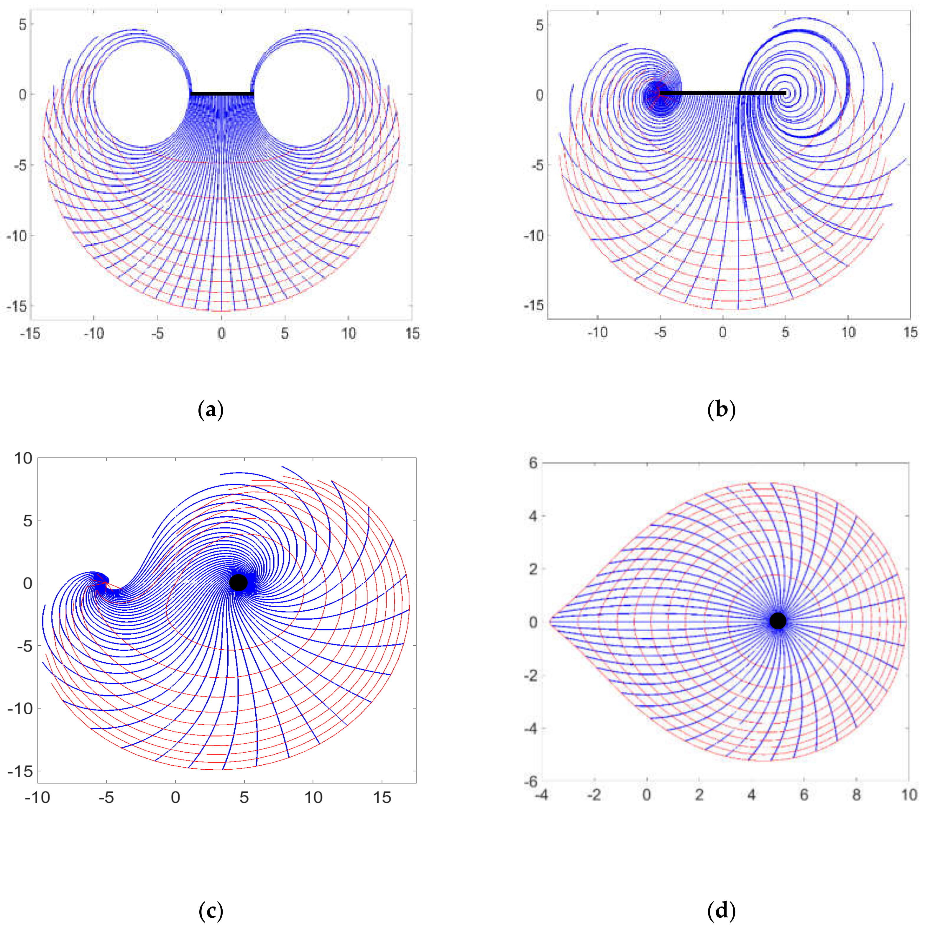
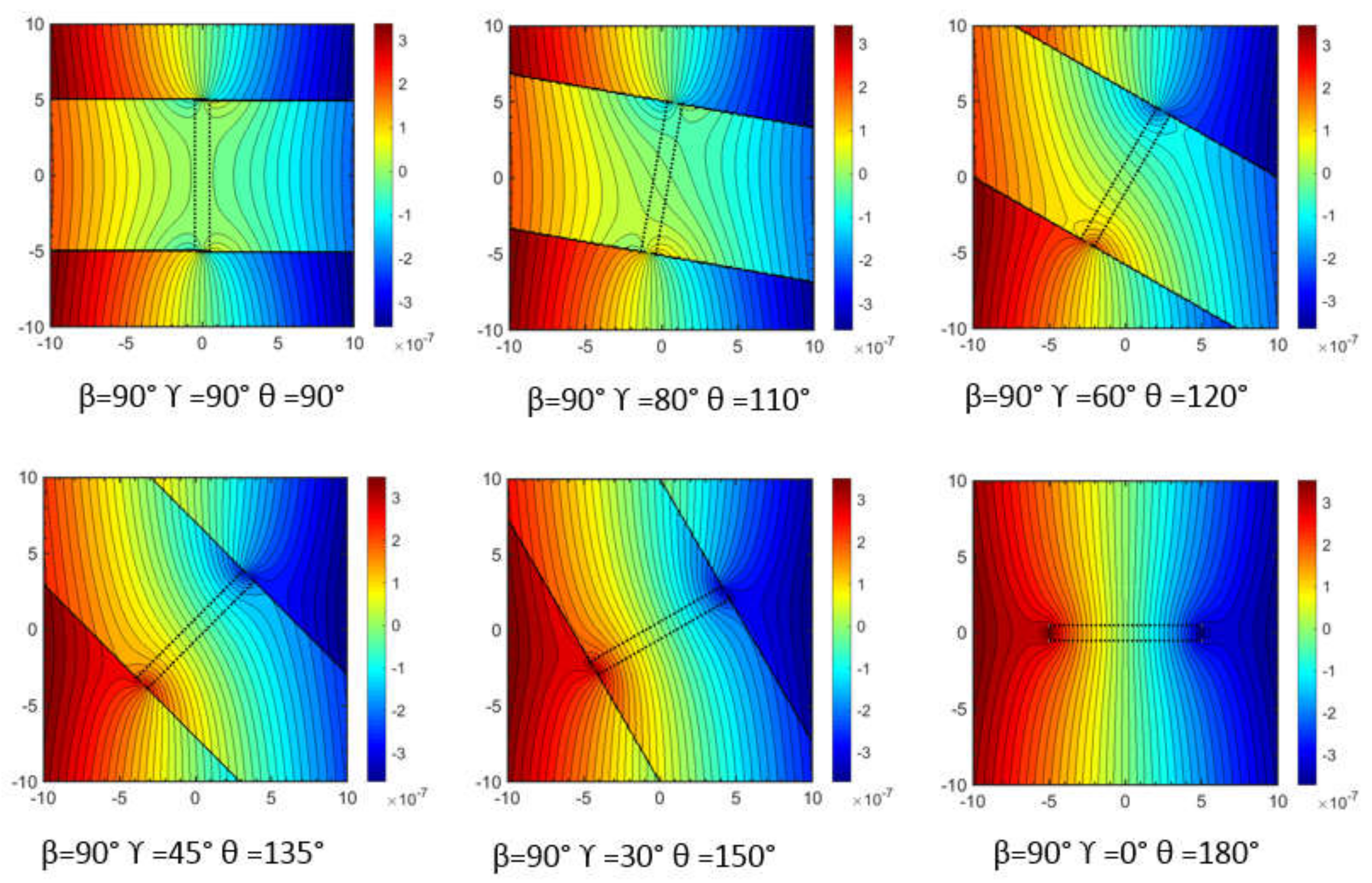
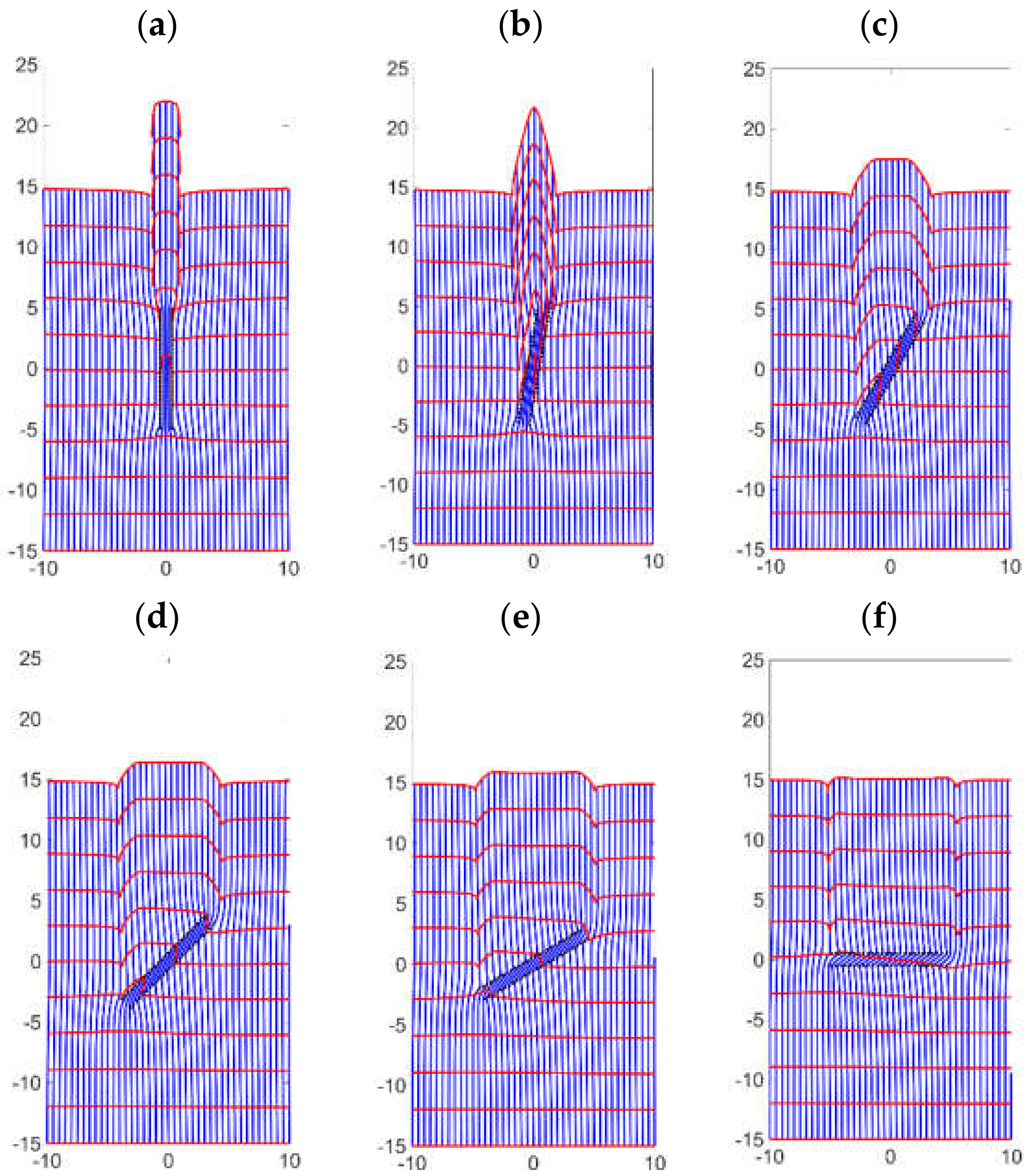
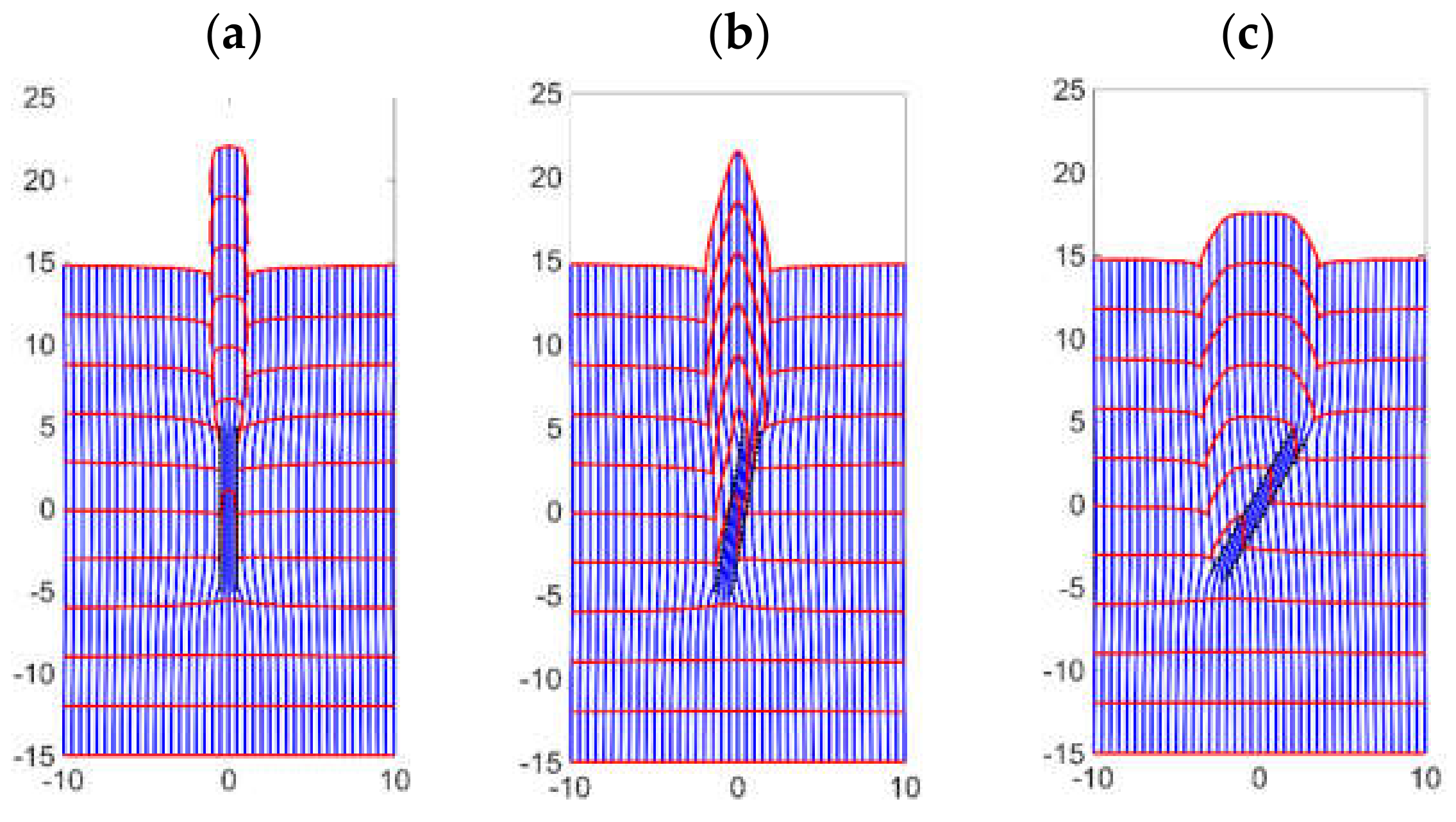
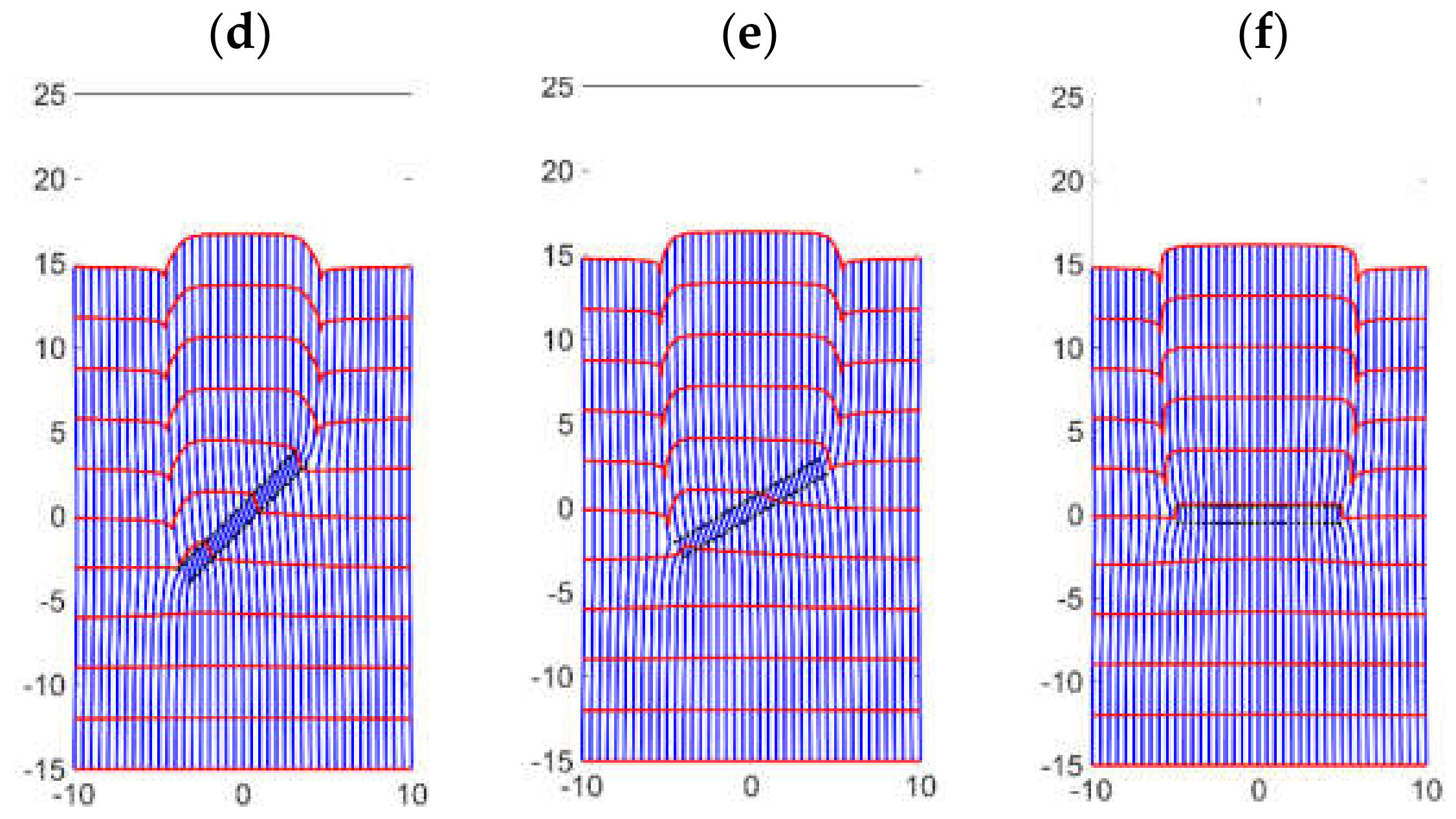
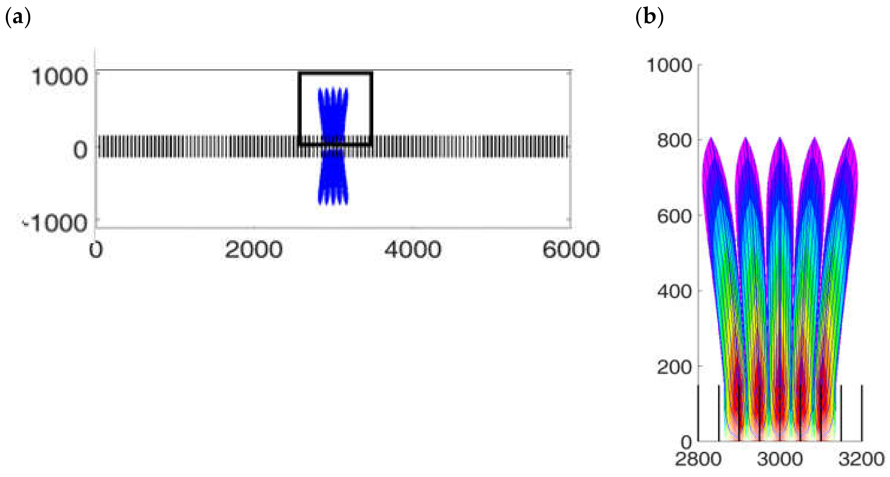
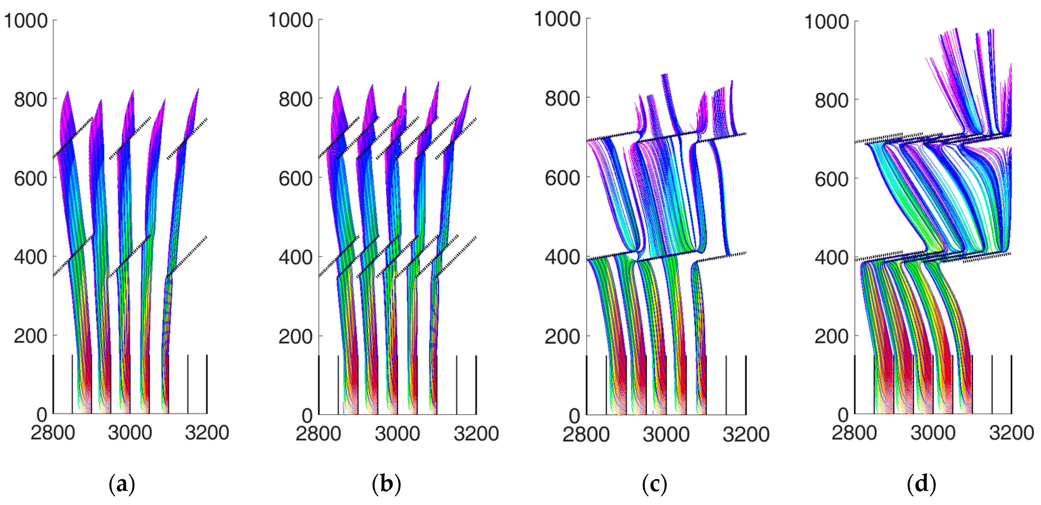
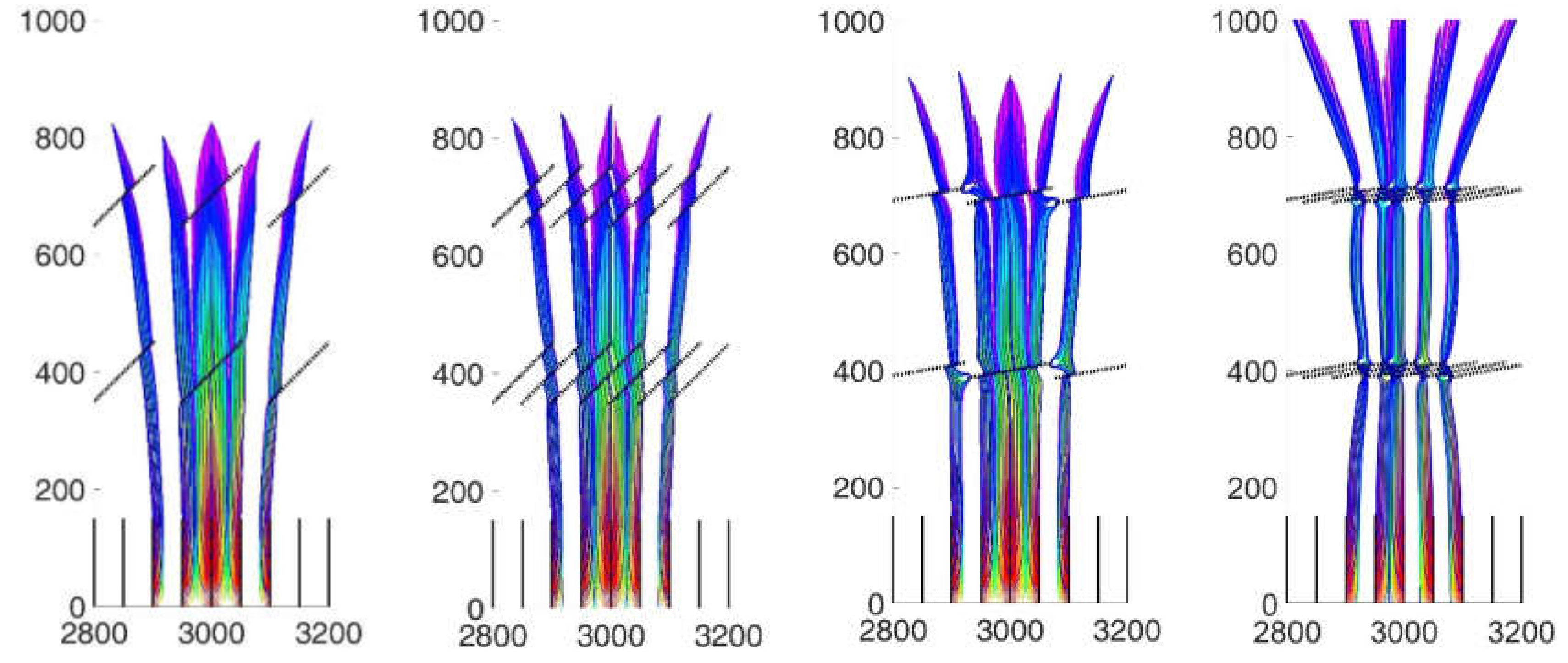
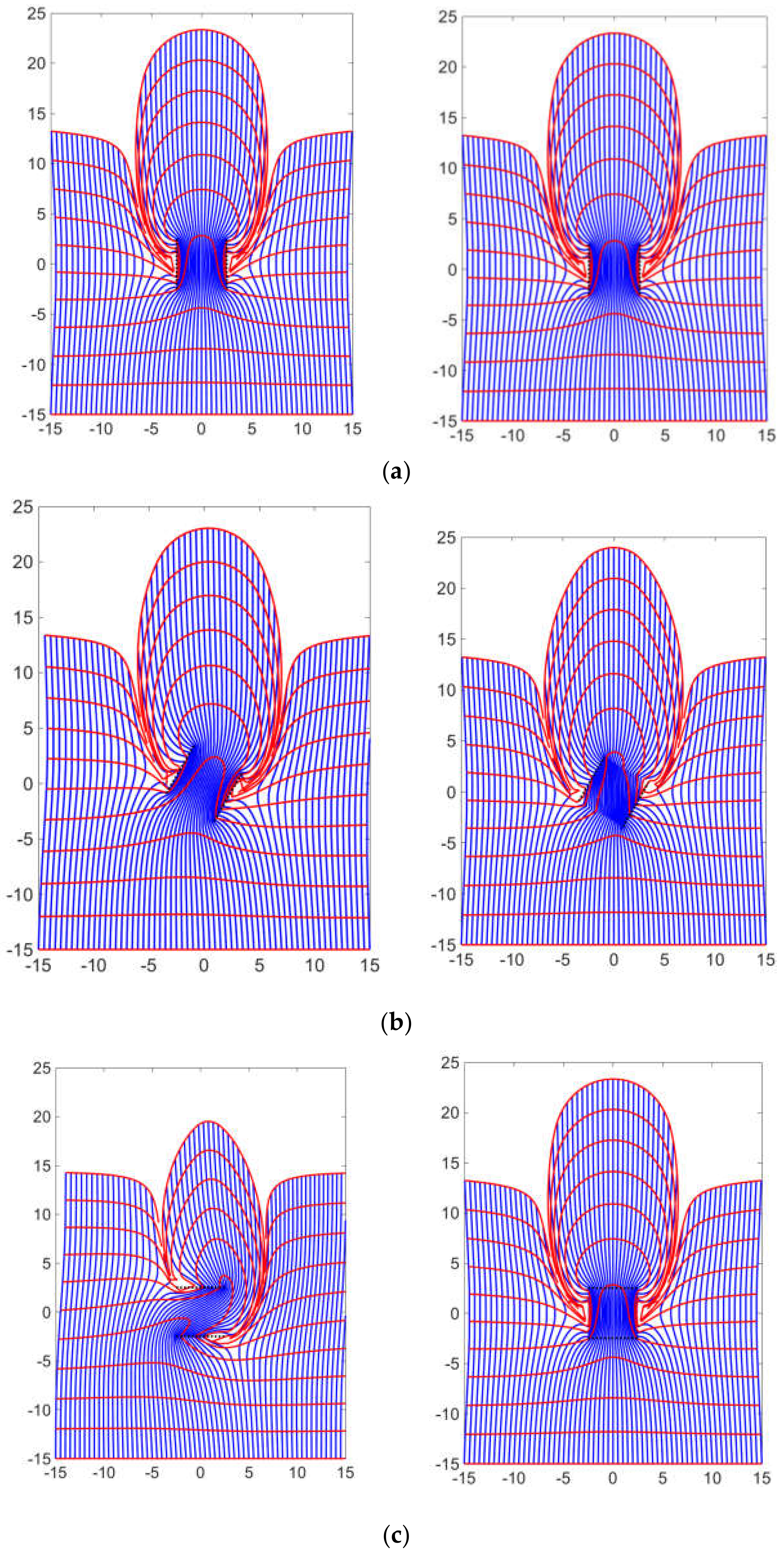
• Areal doublets can be used to model the flow in high conductivity flow channels such as the natural fractures in porous media. The natural fractures (areal doublets) distort the DRV and locally increase the velocity while modeling the flow in porous media (Figure 16).
• The modified areal doublet algorithm in Equation (12) yields a more realistic result for fractures oriented at a high angle with respect to the direction of fluid flow (Figure 16d).
• The augmented solution in the present study avoids the branch cuts and therefore provides an efficient method to model the flow paths of fluids in naturally fractured porous media.

References

1. Karimi-Fard, M.; Durlofsky, L.J.; Aziz, K. An efficient discrete-fracture model applicable for general-purpose reservoir simulators. Soc. Pet. Eng. 2004. [Google Scholar] [CrossRef]
2. Moridis, G.J.; Blasingame, T.A.; Freeman, C.M. Analysis of mechanisms of flow in fractured tight-gas and shale-gas reservoirs. In Proceedings of the SPE Latin American and Caribbean Petroleum Engineering Conference, Lima, Peru, 1–3 December 2010. [Google Scholar] [CrossRef] [Green Version]
3. Olorode, O.; Freeman, C.M.; Moridis, G.; Blasingame, T.A. High-resolution numerical modeling of complex and irregular fracture patterns in shale-gas reservoirs and tight gas reservoirs. SPE Reserv. Eval. Eng. 2013, 16. [Google Scholar] [CrossRef]
4. Sun, J.; Hu, K.; Wong, J.; Hall, B.; Schechter, D. Investigating the effect of improved fracture conductivity on production performance of hydraulic fractured wells through field case studies and numerical simulations. Soc. Pet. Eng. 2014. [Google Scholar] [CrossRef]
5. Van Harmelen, A.; Weijermars, R. Complex analytical solutions for flow in hydraulically fractured hydrocarbon reservoirs with and without natural fractures. Appl. Math. Model. 2018, 56, 137–157. [Google Scholar] [CrossRef]
6. Khanal, A.; Weijermars, R. Modeling flow and pressure fields in porous media with high conductivity flow channels and smart placement of branch cuts for variant and invariant complex potentials. Fluids 2019, 4, 154. [Google Scholar] [CrossRef] [Green Version]
7. Weijermars, R.; van Harmelen, A.; Zuo, L. Controlling flood displacement fronts using a parallel analytical streamline simulator. J. Pet. Sci. Eng. 2016, 139, 23–42. [Google Scholar] [CrossRef]
8. Strack, O.D.L. Groundwater Mechanics; Prentice-Hall: Englewood Cliffs, NJ, USA, 1989. [Google Scholar]
9. Weijermars, R.; van Harmelen, A. Breakdown of doublet re-circulation and direct line drives by far-field flow: Implications for geothermal and hydrocarbon well placement. Geophys. J. Int. 2016, 206, 19–47. [Google Scholar] [CrossRef] [Green Version]
10. Holzbecher, E. Streamline visualization of potential flow with branch cuts, with applications to groundwater. J. Flow Vis. Image Process. 2018, 25, 119–144. [Google Scholar] [CrossRef]
11. Walton, I.; Mclennan, J. The role of natural fractures in shale gas production. Eff. Sustain. Hydraul. Fract. 2013, 327–356. [Google Scholar] [CrossRef]
12. Aguilera, R. Effect of fracture compressibility on gas-in-place calculations of stress-sensitive naturally fractured reservoirs. SPE Reserv. Eval. Eng. 2008, 11, 307–310. [Google Scholar] [CrossRef]
13. Kolawole, O.; Ispas, I. Interaction between hydraulic fractures and natural fractures: Current status and prospective directions. J. Petrol. Explor Prod. Technol. 2019. [Google Scholar] [CrossRef] [Green Version]
14. Yang, X.; Yu, W.; Wu, K.; Weijermars, R. Assessment of production interference level due to fracture hits using diagnostic charts. Soc. Pet. Eng. 2020. [Google Scholar] [CrossRef]
15. Weijermars, R.; Van Harmelen, A. Advancement of sweep zones in waterflooding: Conceptual insight and flow visualizations of oil-withdrawal contours and waterflood time-of-flight contours using complex potentials. J. Pet. Explor. Prod. Technol. 2017, 7, 785–812. [Google Scholar] [CrossRef] [Green Version]
16. Khanal, A.; Weijermars, R. Visualization of drained rock volume (DRV) in hydraulically fractured reservoirs with and without natural fractures using complex analysis methods (CAMs). Pet. Sci. 2019, 16, 550–577. [Google Scholar] [CrossRef] [Green Version]
17. Olson, J.E. Multi-fracture propagation modeling: Applications to hydraulic fracturing in shales and tight gas sands. In Proceedings of the the 42nd U.S. Rock Mechanics Symposium (USRMS), San Francisco, CA, USA, 1 January 2008. [Google Scholar]
18. Cipolla, C.L.; Lewis, R.E.; Maxwell, S.C.; Mack, M.G. Appraising unconventional resource plays: Separating reservoir quality from completion effectiveness. In Proceedings of the International Petroleum Technology Conference, Bangkok, Thailand, 1 January 2011. [Google Scholar] [CrossRef]
19. Warren, J.E.; Root, P.J. The behavior of naturally fractured reservoirs. Soc. Pet. Eng. J. 1963, 3, 245–255. [Google Scholar] [CrossRef] [Green Version]
20. Kazemi, H.; Merrill, L.S., Jr.; Porterfield, K.L.; Zeman, P.R. Numerical simulation of water-oil flow in naturally fractured reservoirs. SPE J. 1976, 6, 317–326. [Google Scholar] [CrossRef]
21. March, R.; Elder, H.; Doster, F.; Geiger, S. Accurate dual-porosity modeling of co2 storage in fractured reservoirs. In Proceedings of the 2017 SPE Reservoir Simulation Conference, Montgomery, TX, USA, 20–22 February 2017. [Google Scholar] [CrossRef]
22. Geiger, S.; Matthai, S.K.; Niessner, J.; Helmig, R. Black-oil simulations for three-component, three-phase flow in fractured porous media. SPE J. 2009. [Google Scholar] [CrossRef]
23. Moinfar, A.; Varavei, A.; Sepehrnoori, K.; Johns, R.T. Development of an efficient embedded discrete fracture model for 3D compositional reservoir simulation in fractured reservoirs. SPE J. 2014, 19, 289–303. [Google Scholar] [CrossRef] [Green Version]
24. Parsegov, S.G.; Nandlal, K.; Schechter, D.S.; Weijermars, R. Physics-driven optimization of drained rock volume for multistage fracturing: Field example from the Wolfcamp formation, Midland Basin. In Proceedings of the Unconventional Resources Technology Conference, Houston, TX, USA, 23–25 July 2018. [Google Scholar] [CrossRef] [Green Version]
25. Weijermars, R.; Khanal, A. High-resolution streamline models of flow in fractured porous media using discrete fractures: Implications for upscaling of permeability anisotropy. Earth-Sci. Rev. 2019, 194, 399–448. [Google Scholar] [CrossRef]
26. Weijermars, R.; Khanal, A.; Zuo, L. Fast models of hydrocarbon migration paths and pressure depletion based on complex analysis methods (CAM): Mini-review and verification. Fluids 2020, 5, 7. [Google Scholar] [CrossRef] [Green Version]
27. Zuo, L.; Weijermars, R. Rules for flight paths and time of flight for flows in heterogeneous isotropic and anisotropic porous media. Geofluids 2017, 2017, 5609571. [Google Scholar] [CrossRef] [Green Version]
28. Weijermars, R. Improving well productivity—Ways to reduce the lag between the diffusive and convective time of flight in shale wells. J. Pet. Sci. Eng. 2020, in press. [Google Scholar]
Figure 1. (ac) Waterfront advance between a series of injector outlets and producer wells in streamline visualizations (left column; yellow flow paths inside grey injection water body; blue curves beyond injection water body). Time-of-flight contours (TOFCs, red curves). Velocity field magnitude (right), scaled by a Bernoulli pressure proxy using the natural logarithm and inverse tangent, outlines the regions (blue) where the fastest flow occurs. Reproduced with permission from [7].
Fluids 05 00051 g001
Figure 2. Conceptual models of: (a) line doublet obtained by superposing an infinite number of singularity doublets; (b) line dipole obtained by superposing an infinite number of singularity dipoles. Reproduced with permission from [5].
Fluids 05 00051 g002
Figure 3. Stream function solutions (in left column) with streamlines for line doublets/line dipoles, based on Equation (1), for a range of polarity angles: (a) θ = 90 ° , (b) θ = 45 ° , (c) θ = 10 ° , and (d) θ = 0 ° . The tilt angle β = 0 ° for all cases. Stream function values ( ψ ) given by rainbow colors (m2·s−1) relative to line y = 0. Potential function solutions are shown in the right column.
Fluids 05 00051 g003
Figure 4. Streamlines (blue) and time-of-flight contours (red) for the line doublet of Equation (1), for a range of polarity angles: (a) θ = 90 ° , (b) θ = 45 ° , (c) θ = 10 ° , and (d) θ = 0 ° , and a tilt angle β = 0 ° based on particle tracking method of Equations (3a,b) and (4a,b). The initial position of the tracked particles is shown in black color. For case (a) and (b) straight lines of length 5 (from −2.5 to 2.5 in x-axis) and 10 m (from −5 to 5 in x-axis) are tracked. For case (c) and (d), particles initially arranged on a minuscule circle with a radius of 0.01 m (located at 5 m from origin in x-axis) are tracked. Cases a-c are simulated for a period of 100 s whereas case d is simulated for 10 s both with a step-size of 0.0001 s.
Fluids 05 00051 g004
Figure 5. Conceptual models of: (a) areal doublet obtained by superposing an infinite number of line doublets; (b) areal dipoles obtained by superposing an infinite number of line dipoles. Reproduced with permission from [6].
Fluids 05 00051 g005
Figure 6. Conceptual model of areal doublet obtained by superposing an infinite number of line doublets. Reproduced with permission from [6]. The angles of tilt angle of γ , corner point angle of β , and polarity angle θ of doublet/dipole singularity in line arrays, located at center z c , and with width W (m), and length of L (m), and za1, za2, za3, and zb2 are the corners of the flow element. The ∞-shaped circulation pattern shows the orientation of the doublet singularities in the line array. Angles are all measured anticlockwise.
Fluids 05 00051 g006
Figure 7. Stream function solution and streamlines for line doublet/line dipole of Equation (9), for a range of polarity angles: (a) θ = 90 ° , (b) θ = 80 ° , (c) θ = 70 ° , (d) θ = 45 ° , (e) θ = 30 ° , and (f) = θ = 10 ° , with a tilt angle for the line doublet element β = 90 ° . Stream function values ( ψ ) given by rainbow colors (m2·s−1) relative to line y = 0. Branch cuts appear at the fracture tips. Solved using the imaginary part of Equation (8).
Fluids 05 00051 g007
Figure 8. Stream function solutions for the areal doublet/line dipole of Equation (9), based on the integral method.
Fluids 05 00051 g008
Figure 9. Particle path solutions showing streamlines (blue) and time of flight contours (red) for a range of inclination angles, based on the Eulerian particle path tracking method: (a) γ = 90 ° , (b) γ = 80 ° , (c) γ = 60 ° , (d) γ = 45 ° , (e) γ = 30 ° , and (f) = γ = 0 ° ; keeping β = θ = 90 ° . The far-field velocity and the strength of the areal doublet/dipole element (adjusted for a porosity of 0.1) is 3.12 × 10⁻⁸ m/s and 3.12 × 10⁻⁷ m2/s respectively.
Fluids 05 00051 g009
Figure 10. Stream function and streamlines solution for areal doublet representation for vertical and horizontal fracture elements. (a) Vertical fracture element, with a far-field flow, and (c) without a far-field flow superposed. (b) Horizontal fracture element, with a far-field flow, and (d) without a far-field flow superposed. Stream function values ( ψ ) given by rainbow colors (m2·s−1) relative to line y = 0. Solved using Equation (5).
Fluids 05 00051 g010
Figure 11. Stream function and streamlines solution for areal dipole of Figure 5c,d. (a,b) With a far-field flow, and (c,d) without a far-field flow superposed. Stream function values ( ψ ) given by rainbow colors (m2·s−1) relative to line y = 0. Solved using Equation (11).
Fluids 05 00051 g011
Figure 12. Areal doublet oriented in two extreme directions [parallel (left) and normal (right) to the far-field flow] are combined to generate the superposed augmented solution. When the element is parallel to flow (such as the first set of vertices in the left image), only the vertical element contributes. When the element is normal to the flow (right image), only the horizontal element contributes. For intermediate elements, sine angles are used to “mix” the appropriate “contribution” of each element. For the first case L = 10, W = 1 and θ = 90°, for the second case L = 1 m, W = 10 m, and θ = 0°.
Fluids 05 00051 g012
Figure 13. Particle path solutions showing streamlines (blue) and time of flight contours (red) for the line doublet/line dipole of Equation (12), for a range of inclination angles, based on the Eulerian particle path tracking method: (a) γ = 90 ° , (b) γ = 80 ° , (c) γ = 60 ° , (d) γ = 45 ° , (e) γ = 30 ° , and (f) γ = 0 ° . The length and the width of the areal doublet/dipole element are 10 m and 1 m respectively. The far-field velocity and the strength of the areal doublet/dipole element adjusted for a porosity of 0.1 is 3.12 × 10⁻⁸ m/s and 3.12 × 10⁻⁷ m2/s respectively.
Fluids 05 00051 g013aFluids 05 00051 g013b
Figure 14. (a). Top view of the full-scale model (horizontal map view) of a well with 119 transverse hydraulic fractures with a fracture half-length of 150 ft (45.7 m). Each hydraulic fracture is assumed to be identical and producing at a constant rate of 13.6 ft3/day (0.39 m3/day) for 30 years. (b). Time of flight contours, represented by the rainbow colors, showing the drainage at each three-year interval of around five hydraulic fractures in the central portion of the well. Reproduced with permission from [16].
Fluids 05 00051 g014
Figure 15. Top view of central five hydraulic fractures for central stage in the well of Figure 14a, with DRV distortion due to (a) six nearby natural fractures, with a strength of 6 × 103 ft4/day (51.8 m4/day) each, at an angle of 45°. (b) As (a), but with 14 natural fractures. (c) Six natural fractures, with a strength of 60 × 103 ft4/day (518 m4/day) each, at an angle of 10°. (d) As (c), but with 14 natural fractures. Time of flight contours (multicolored) show the drainage at each three-year interval. Reproduced with permission from [8].
Fluids 05 00051 g015
Figure 16. Same as Figure 15a–d, but generated with the augmented solution of Equations (12)–(18).
Fluids 05 00051 g016
Figure 17. Particle path solutions showing streamlines (blue) and time of flight contours (red) for the line doublet/line dipole of Equation (5) (left column) and Equation (12) (right column), for a range of inclination angles, based on the Eulerian particle path tracking method: (a) γ = 90 ° , (b) γ = 60 ° , (c) γ = 0 ° . The length and width of the areal doublet/dipole elements are 5 m × 5 m, respectively. The far-field velocity and the strength of the areal doublet/dipole element adjusted for a porosity of 0.1 are 3.12 × 10⁻⁸ m/s and 2.97 × 10⁻⁶ m2/s, respectively.
Fluids 05 00051 g017