Article

Numerical Simulation of Velocity Field around Two Columns of Tandem Piers of the Longitudinal Bridge

1
Key Laboratory for Special Area Highway Engineering of Ministry of Education, Chang’an University, Xi’an 710064, Shaanxi, China
2
Department of Civil, Construction and Environmental Engineering, Iowa State University, Ames, IA 50011, USA
*
Author to whom correspondence should be addressed.
Fluids 2020, 5(1), 32; https://doi.org/10.3390/fluids5010032
Submission received: 29 December 2019 / Revised: 2 March 2020 / Accepted: 7 March 2020 / Published: 12 March 2020
(This article belongs to the Special Issue Recent Numerical Advances in Fluid Mechanics, Volume II)

Abstract

:
This research explores the effects of different spans of two columns of tandem piers on the characteristics of x-velocity near the river bed based on computational fluid dynamics (CFD) simulations. With a span shorter than 27.5D (D is the diameter of piers), the shape and the lateral range of the x-velocity increases with the increase of distance downwards the x-direction. For the area between the tandem piers and the wall, the VRi/VR1 (the ratio of the x-velocity at the i-th row to the x-velocity of the first row in each model) near the wall increases up to 1.26. For the area between the two columns of tandem piers, the profile of VRi/VR1 changes from a “∩-shape” to an “M-shape” in each model. RAVC (average velocity change ratio) of different spans increases gradually and tends to be stable with the increases of the span. The largest RAVC is about −17.66% with a span of 0.52 m. The RMV (the ratio of the maximum x-velocity among piers in each row in different models to the maximum x-velocity of the two piers arranged side by side) of piers in the first row of different models is around 0.95. The RMV becomes 0.82 at the second pier in each model when the span is shorter than 27.5D, and increases to 0.91 if the span is longer than 27.5D. If the span is longer than 27.5D, the RMV of different piers are close to each other from the 2nd pier to the last one.

1. Introduction

In the past two decades, many highways have been constructed in China, especially in the western mountainous areas. To minimize the effects of highway infrastructures on the local environment and biological systems, longitudinal bridges are more frequently adopted. Unlike the conventional bridges that are cross over the river, the longitudinal bridges are built in the river and extended along the river. This eliminates building embankment and tunnels that cause significant effects on the local environment. For example, the Xi’an-Hanzhong highway of China contained nearly 10 km of longitudinal bridges as shown in Figure 1. However, tandem piers of longitudinal bridges are distributed in the riverbed, which significantly disturbs river flow fields and causes soil erosion and scour. For example, half a year after the Xi’an-Hanzhong highway was opened to the public on September 2007, many longitudinal bridges of the Xi’an-Hanzhong highway have found severe scour issues as shown in Figure 2, which affected the foundation safety of bridges.
Many experimental and numerical studies have investigated flow fields around a bridge pier and pier groups [1,2,3]. Lin et al. [4] investigate the flow field around two cylinders. Tian et al. [5] studied the flow characteristics around a cylinder pier. He et al. [6] studied the effects of piers on the flow field. Li et al. [7] studied the influence of pier configuration on the field around the bridge. Kim et al. [8] investigated the flow between a pair of cylinders in the flopping region. Gu [9] studied the interference between two circular cylinders at supercritical Reynolds number. Sumner et al. [10] studied the flow-pattern identification for two staggered circular cylinders in cross-flow. Meneghini et al. [11] studied the flow interference between two circular cylinders in tandem and side-by-side configurations. Li et al. [12] measured the average velocity, vertical velocity, and distribution of the velocity of a variety of different pile groups in a rectangular open channel. Ataie-Ashtiani et al. [13] studied the velocity field around side-by-side piers with and without a scour hole. Yan et al. [14] studied the velocity distribution of bridge piers with different intersection angles between bridge axle and flow direction.
For piers arranged in tandem, researchers have investigated the effects of pile space on the vortex shedding frequencies. Igarashi [15] studied the characteristics of the flow around two circular cylinders arranged in tandem. Mahbub et al. [16] studied the relationship between strouhal numbers, forces, flow structures around two tandem cylinders, and the diameters. Ataie-Ashtiani et al. [17] performed experiments to investigate the flow pattern around tandem piers in a flat fixed moderately rough using an Acoustic Doppler Velocimeter under clear water conditions. The results showed that the presence of the downstream pier changes the flow structure greatly, particularly in the near wake region. Reynolds number, bed roughness, and pier spacing can influence the type of flow regime of the tandem piers. Wang et al. [18] studied the local scouring around three piers in a tandem arrangement in clear water conditions. Chavan et al. [19] studied the flow and scour characteristics around tandem piers in sandy channels with downward seepage. Beg et al. [20] studied the scour characteristics of two unequal size bridge piers in tandem arrangement. The relevant research results are shown in Table 1.
With the development of computer science, numerical simulations based on Computational Fluid Dynamics (CFD) codes (e.g., Flow-3D(Three-Dimensional), Fluent) have been wildly used. The simulation results have been proved to be consistent with experimental results [21,22,23,24,25,26,27,28,29,30]. For tandem piers, Palau-Salvador et al. [31] conducted numerical simulations around two submerged tandem piers and presented flow streamlines at different planes. Mohamed [32] studied the flow and local scour at two submerged-emergent tandem cylindrical piers by numerical simulation.
Bridge piers affect the characteristics of the flow field, such as the velocity. The effects of tandem piers on the flow field are more complicated. The goal of this study is to investigate the flow field around the tandem piers and explore the effects of the different spans of tandem piers on the velocity characteristics based on Flow-3D. This may provide the characteristics of the velocity field near-bed region around two columns of tandem piers of the longitudinal bridge.

2. Model Setup

Flow-3D employs numerical techniques to solve the fluid motion equations to obtain transient three-dimensional solutions to multi-scale, multi-physics flow problems [33,34,35,36]. FLOW-3D contains a simple, fast, yet powerful meshing capability through the Fractional Area/Volume Obstacle Representation (FAVOR), which is used to illustrate the complex boundaries of the solution domain. Flow-3D also allows several turbulences closure schemes to be incorporated and tested. These closure schemes include simple eddy viscosity, one-dimensional Prandtl mixing length, two-equation k-e, large-eddy, and four-equation Re-Normalized Group (RNG) models. Flow-3D focuses on the free surface and multi-phase applications, serving a broad range of industries including open channel hydraulics, water civil infrastructure, microfluidics, and bio-medical devices [37,38,39]. The Volume of Fluid (VOF) is a typical model to track the water surface for solving the nonlinear Navier-Stokes equation in Flow-3D, and especially for applying on the liquid motion. Furthermore, it was used to investigate the vortex in a box test to calculate the volume tracking algorithm. In addition, the FAVOR method is used to compute the zone of flow obstacles and demonstrate the boundaries of the domain.

2.1. Governing Equations in the Hydrodynamic Model

Fluid motion equations include the continuity equation and momentum equations. Continuity equation, momentum equations, and the Volume of the Fluid equation in the Cartesian coordinate system are shown as follows:
Continuity V F ρ t + x ( ρ u A x ) + R y ( ρ v A y ) + z ( ρ w A z ) = R S O R
X - momentum   u t + 1 V F ( u A x u x + v A y R u y + w A z u z ) ξ A y v 2 x V F = 1 ρ ρ x + G x + f x
Y - momentum   v t + 1 V F ( u A x v x + v A y R v y + w A z v z ) ξ A y u v x V F = R ρ ρ y + G y + f y
Z - momentum   w t + 1 V F ( u A x w x + v A y R w y + w A z w z ) = 1 ρ ρ z + G z + f z b z
V F F t + ( A U F ) = 0
where VF is the open volume ratio to flow, ρ is the fluid density, (u, v, w) is the velocity components in x, y, and z direction, respectively, RSOR is the source function, (Ax, Ay, Az) is the fractional areas, (Gx, Gy, Gz) is the gravitational force, (fx, fy, fz) is the viscosity acceleration, and (bx, by, bz) is the flow losses in porous media in x, y, z directions, respectively. The right side of equations 2 to 4 show mass injection when the velocity is 0. In equation 5, A is the average of area flow, U is the average velocity in (x, y, z) direction, and F is volume fluid function. When the cell is full of fluid, the F is one, and F is zero when the cell is empty. In FLOW-3D, two methods are used for simulation. The first method is called the Volume of Fluid (VOF) that is used to simulate the fluid at the free surface. The second method is the Fractional Area-Volume Obstacle Representation (FAVOR) method, which is a program used for surface modeling and rigid volumes such as geometric borders.

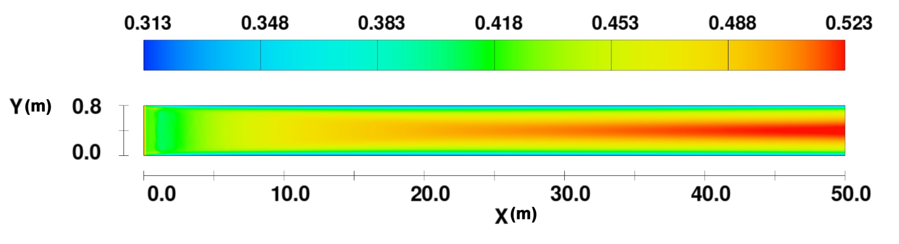
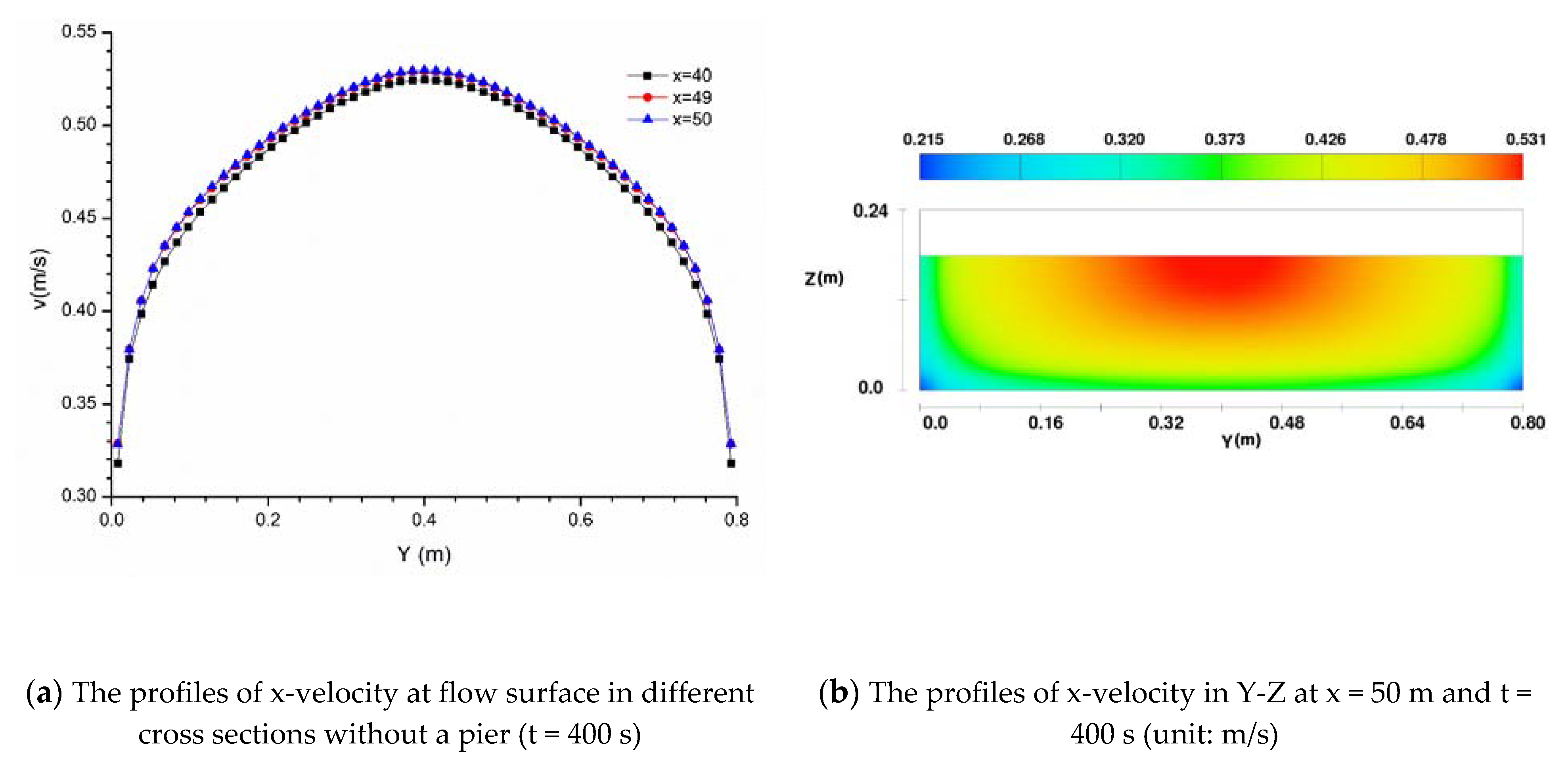
2.2. Model Setup without Piers

There are many factors that influence the flow fields around tandem piers in the longitudinal bridge sections. These factors can be divided into two types: river characteristics and longitudinal bridge characteristics. Based on the field investigation, river channel pattern, the plane of the bridge, the span of piers, layout of piers, and position of piers in the river are selected as the influence factors of longitudinal bridge velocity fields.
This study established the models of river and tandem piers according to the geometry of the longitudinal bridge in Figure 1a. In the field, the diameter of the piers is 1.0 m with a span of 25.0 m. The river was simulated by a normal fixed-bed model. In order to reduce the size of the model, the model scale was set at 1:25. Therefore, the diameter of the bridge pier in the model was 0.04 m. According to the results of Sarker [40] and Breuer [41], in order to reduce the influence of parameters such as calculation domain size and water depth on the calculation results, the width of the calculation domain in this study was considered as 20D (D is the pier diameter) and the initial water depth was set to 4D. Parameters of the model are shown in Table 2.
A numerical model with these parameters was built in FLOW-3D. The water was considered as an incompressible fluid. The viscosity of the water was 0.001 kg/m/s, and the Renormalized Group (RNG) model was utilized. Mesh sizes have great impacts on the accuracy of the results. D/20 (0.2 cm) was set as the grid size based on the suggestions of Sarker [40]. In order to be consistent with the actual situation, the boundary conditions of upstream for calculating must be fully developed. In this study, the flow through a 50-m long channel without a pier was simulated based on the model parameters in Table 1. The boundary conditions of the model are shown in Table 3. As an initial condition, the average velocity was 0.5 m/s.
Simulations showed that the flow rate will be stabilized within 400 s, and the residual (Epsi) of the result meets the requirement (residual is less than 1 × 10⁻²%) and remain stable. Therefore, the calculation time is set as 400 s in this study. The flow field in X-Y at z = 12.75 cm and t = 400 s without a pier is shown in Figure 3. It can be seen that after the water enters the calculation domain, the flow velocity reduces rapidly near the boundaries because of the influence of the wall, where the boundary layer was formed. On the other hand, the flow field in the middle of the channel is almost unaffected. As the flow continues to develop, the influence of the boundary layer becomes more prominent, and the thickness of the boundary layer also increases. Eventually, the velocity in the y direction at a certain cross-section will not change after the flow has fully developed.
The x-velocity at the flow surface in the y direction at different cross-sections in the channel without a pier is shown in Figure 4. The x-velocity distribution in different cross-sections at the flow surface is not changed when x is larger than 49 m as shown in Figure 4a, which indicates that the flow is fully developed in the domain. Therefore, the velocity distribution at x = 50 m (shown in Figure 4b) is used as the boundary conditions of the inlet of the model with piers.

2.3. Model Setup with Piers

2.3.1. Parameters of the Model with Piers

The Xi’an-Hanzhong highway is a four-lane dual carriageway. Some sections of the longitudinal bridges were designed as a separated carriageway, which has two piers with a diameter of 1.0 m, and the lateral distance between the center of piers is 10.50 m. In this study, the span of piers was selected according to the standard span of pier within 50 m specified in the General Specifications for Design of Highway Bridge and Culverts (JTG D60-2015) in China. In addition, the position of the model in the river was indicated by the distance between the centerline of the model and the channel bank. The position of the model in the river is 0.4 m in this study, which means that the center of the model is also the center of the channel. Parameters of the model with piers are shown in Table 4.

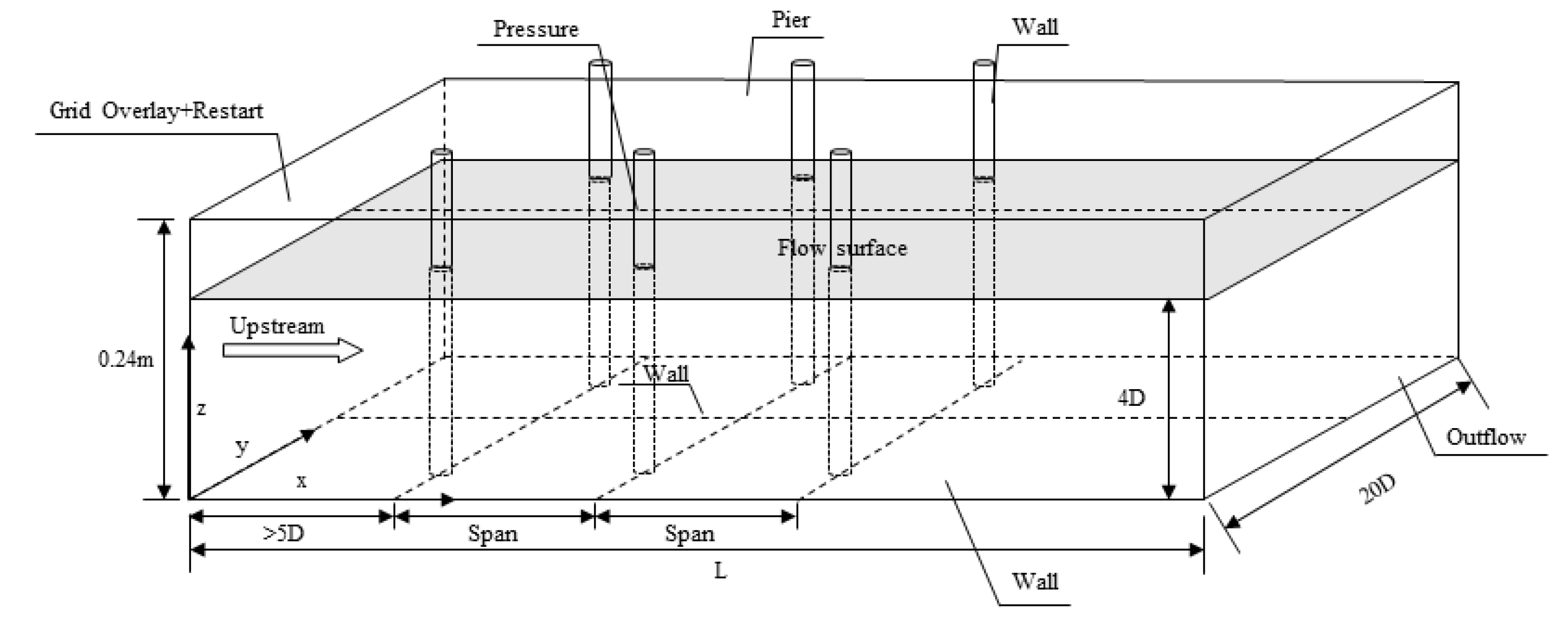
2.3.2. Layout of the Model with Piers

According to the research results of Sarker [40], in order to reduce the influence of parameters such as calculation domain size and water depth on the calculation results, the distance between the inlet and the first pier must be longer than 5D. The length of the domain in the flow direction (L as shown in Figure 5) varies with the span of the piers. This ensures that there are at least four piers in the model. The layout and the boundary conditions of the model with piers are shown in Figure 5.

3. Results and Discussion

3.1. Simulation of each Model

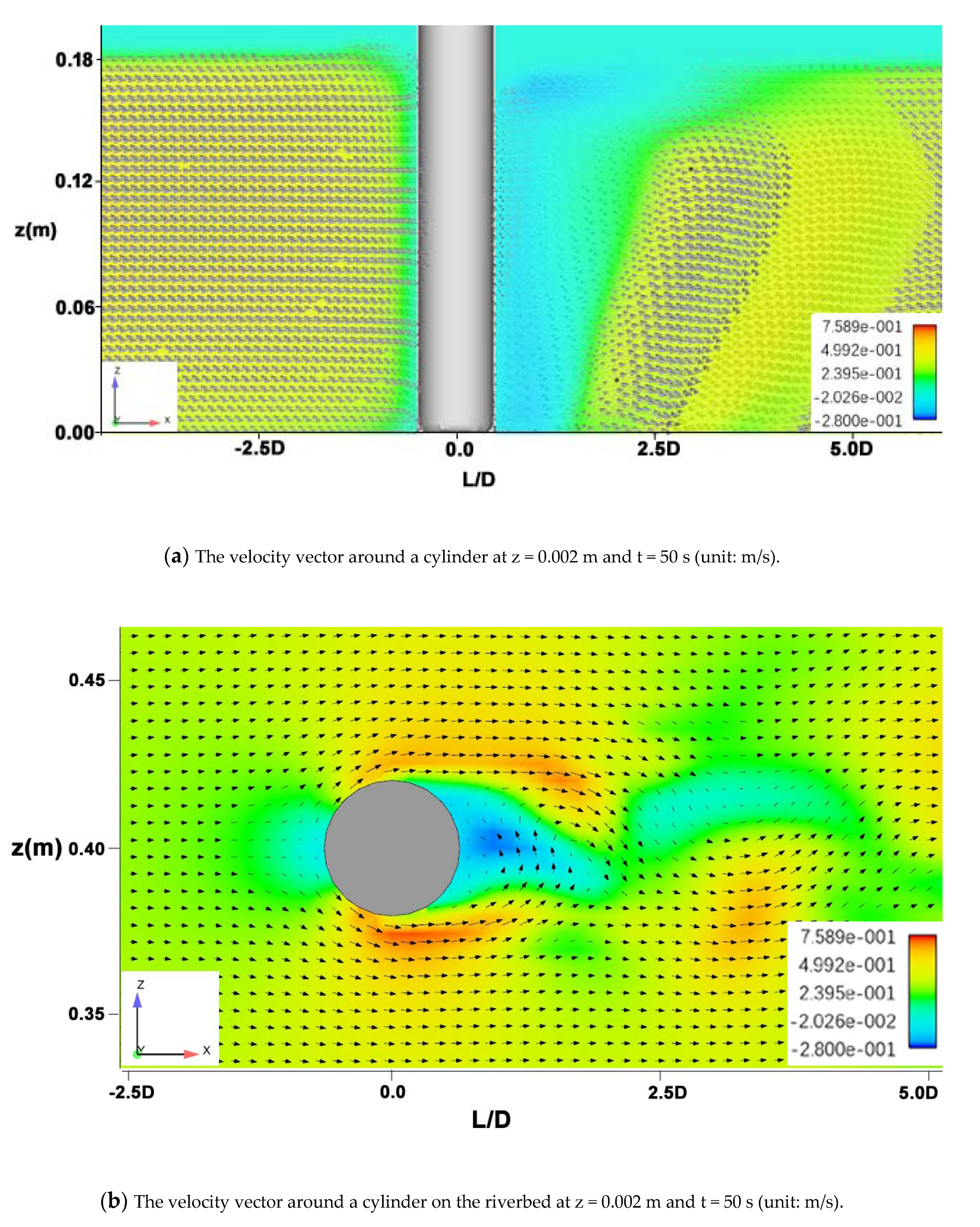
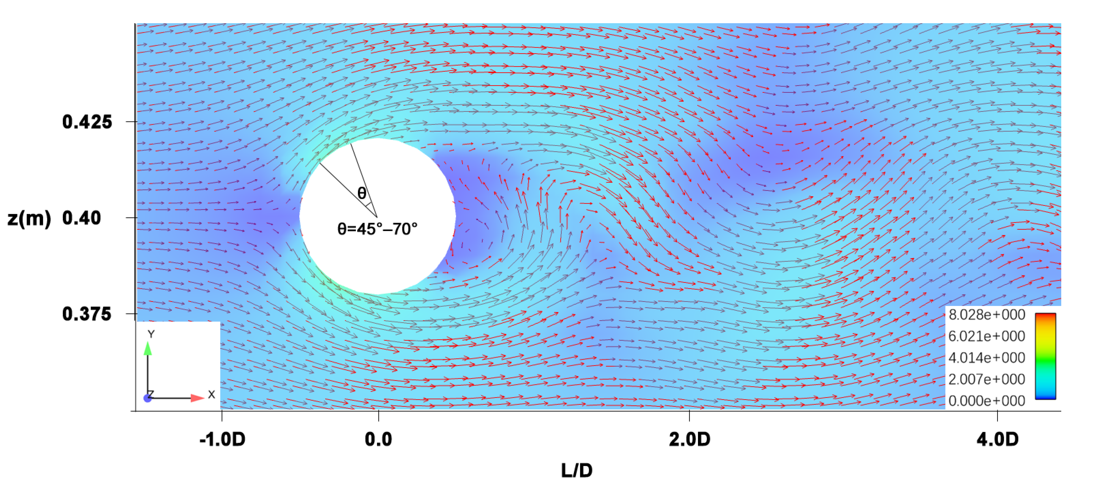
3.1.1. The X-Velocity Field abound Two Piers Arranged Side by Side

In order to verify the accuracy of the simulation results, the velocity field characteristics with two piers arranged side by side were simulated. The layout and the boundary conditions of the model were the same as the model shown in Figure 5, and the piers were located at (x = 50.3 m, y = 0.19 m) and (x = 50.3 m, y = 0.61 m).
The simulation results showed that the flow became stable within 50 s in the calculation domain, and the residuals met the requirement (residual must be less than 1 × 10⁻²%) and remain stable. Therefore, this study used 50 s as the calculation time. The simulation results are analyzed in Figure 6, Figure 7, and Figure 8.
Figure 6a shows the x-velocity in the x-y plane at z = 0.002 m and t = 50 s. The Kármán vortex street is formed when the water flows around the pier, which causes the velocity to change rapidly within a certain length after the pier. As the water flows away from the pier, the influence of the vortex on the velocity reduces and water eventually becomes stable. Figure 6b shows the x-velocity at y = 0.19 m and y = 0.61 m, z = 0.002 m, and t = 50 s. The area affected by the Kármán Vortex Street start from x = 50.3 m to x = 50.74 m, with a length of 0.44 m (11D), followed by a recovery area (or stabilization area) from x = 50.74 m to x = 51.40 m with a length of 0.7 m (16.5D), followed by a stable area after x = 51.40 m (longer than 27.5D).
Roulund [42] pointed out that the flow field around a vertical pile fixed on the bed mainly included the following flow characteristics: the formation of the bottom boundary layer; the formation of the horseshoe vortex in front of the cylinder; the formation of a new boundary layer in front of the cylinder due to the falling flow; the separation of the flow on the side of the cylinder; and the formation of the wake vortex. These characteristics can be observed in Figure 7 and Figure 8 in this study. This validates the effectiveness and accuracy of this simulation methodology in this study.
Figure 7a,b show the zoomed flow field around the pier. We can observe the following characteristics: the horseshoe vortex in front of the pier, the bottom boundary layer, the lateral velocity field, a flow separation on both sides of the pier, and a wake vortex behind the pier. In Figure 7b, the flow separates at about 95° on both sides from the pier, and a weak vortex is formed within 1D behind the pier. Figure 8 shows the excess shear stress field on the river bed surface. It shows the maximum excess shear stress occurs at around 45°–70° (the angle is measured from the main flow direction, as shown in the sector) on the pier side. Referring to the results of Roulund et al. [43], the position of the maximum excess shear stress is where the erosion begins.

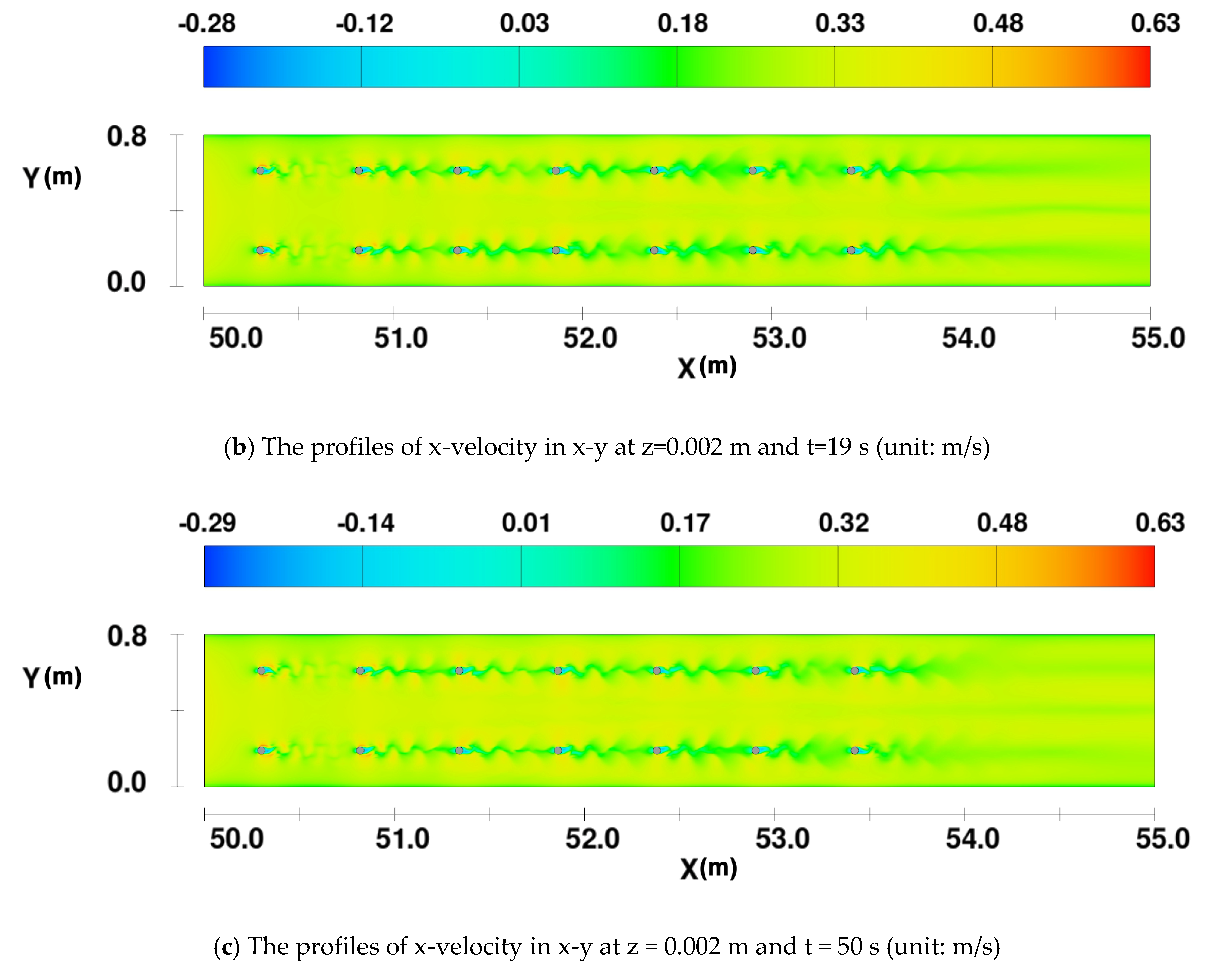
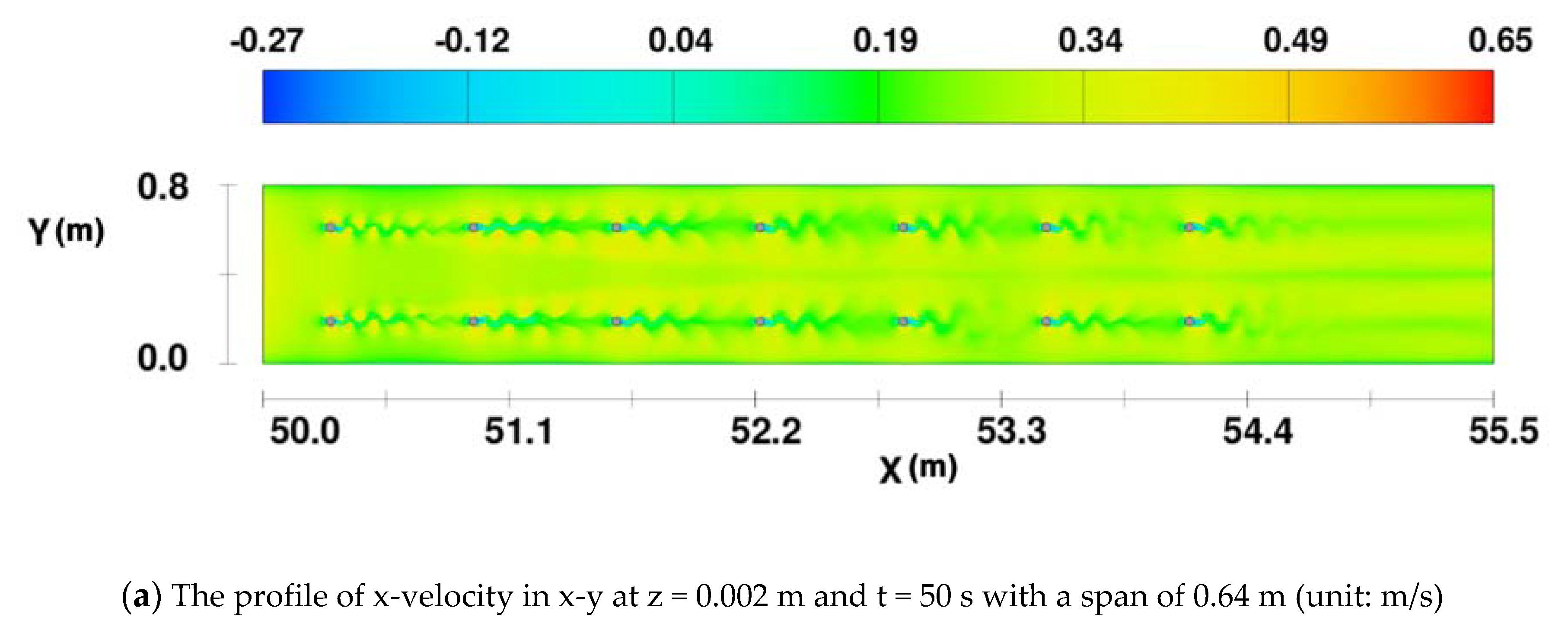
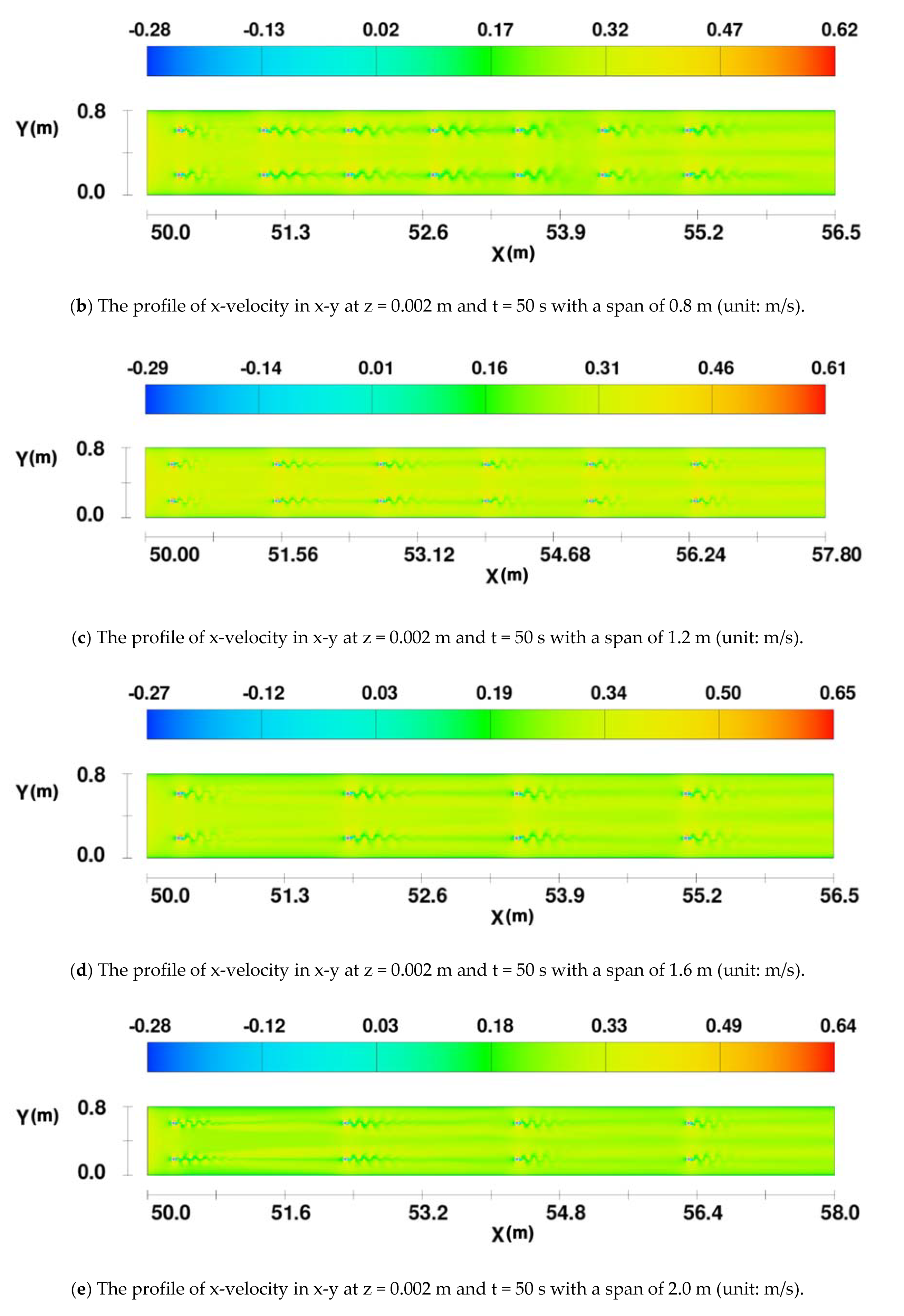
3.1.2. The X-Velocity Field around Two Columns of Tandem Piers of the Longitudinal Bridge

Seven pairs of tandem piers with a span of 0.52 m were built based on the layout and boundary conditions in the river model shown in Figure 5. The same parameter setups were used here. The x-velocity of the riverbed surface (z = 0.002 m) at different times were analyzed in Figure 9a–c. The riverbed was analyzed because the erosion, scour, and siltation occurred at the riverbed, which is critical to the local scour of bridge piers.
At the beginning (t = 4 s), the flow patterns and characteristics around each pier developed individually. Initially, the velocity in front of the pier reduced due to the blocking of water by each pier. The same observation was made when simulating a single pier. When the flow bypassed the pier, the velocity on both sides of the pier increased rapidly, which caused the velocity reaches the maximum value. Many vortices were generated around the pier, which caused a sharp change in velocity. Subsequently, as time increased, a Kármán Vortex Street developed at each pier in turn as shown in Figure 9a. Finally, each of the Kármán Vortex Streets fully developed. The sheltering effect from the upstream piers became stronger. This caused an accumulative effect on the value and distribution of the velocity, except for the velocity near the first pier. Therefore, the size of vortices increases downwards x-direction and becomes stable at t = 50 s as shown in Figure 9b,c. The presence of downstream piers caused an accumulative effect on the flow structure. The velocity decreased in the gap between two piers due to the sheltering effect of the upstream pier. The same observation has been reported by Ataie-Ashtiani et al. [17].
The spans between piers were increased from 0.52 m to 0.64 m, 0.80 m, 1.20 m, 1.60 m, and 2.00 m. The simulations were repeated for each span. Profiles of the x-velocity with different spans in x-y at z = 0.002 m and t = 50 s are shown in Figure 10.
The accumulative influence of the superposition of the Kármán Vortex Streets on the x-velocity was observed when the span was shorter than 27.5D, as shown in Figure 10a,b. Evidently, the shorter span exaggerated the accumulative effects of the superposition of Kármán Vortex Streets. When the span was longer than 27.5D, the accumulative effects were reduced and the x-velocity visually became independent of each other, especially when the span was longer than 2.0 m. That is because if the span was shorter than 27.5D, each pier was located in the recovery area of the Kármán Vortex Street of the previous one. Therefore, the Kármán Vortex Street generated by the previous one had a large influence on the latter pier. If the span was longer than 27.5D, each pier was located in the stable area of the Kármán Vortex Street of the previous pier. Thus, the Kármán Vortex Street generated by the previous one had less or even no influence on the latter pier. As a result, the flow pattern after each pier was independent of each other.

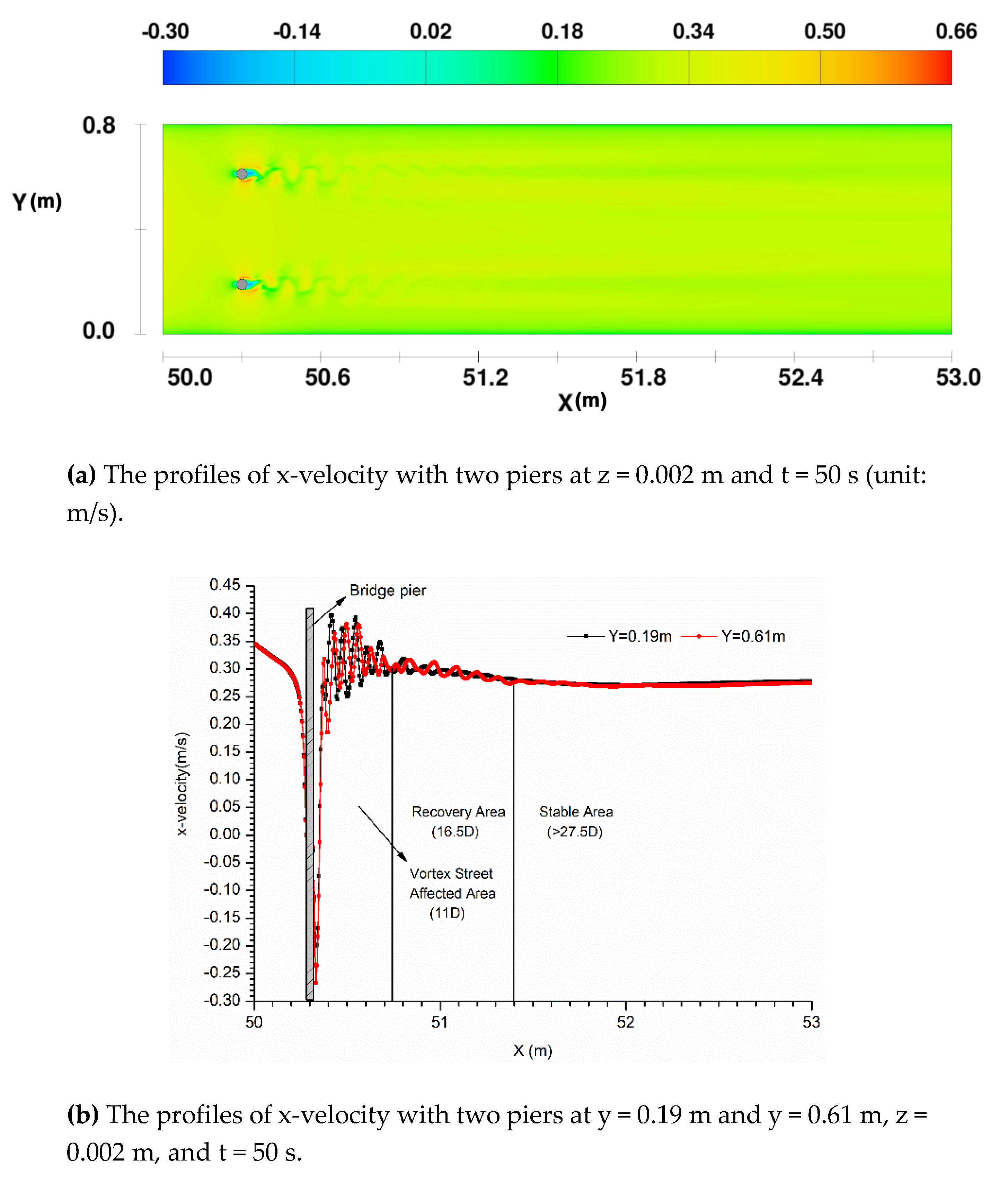
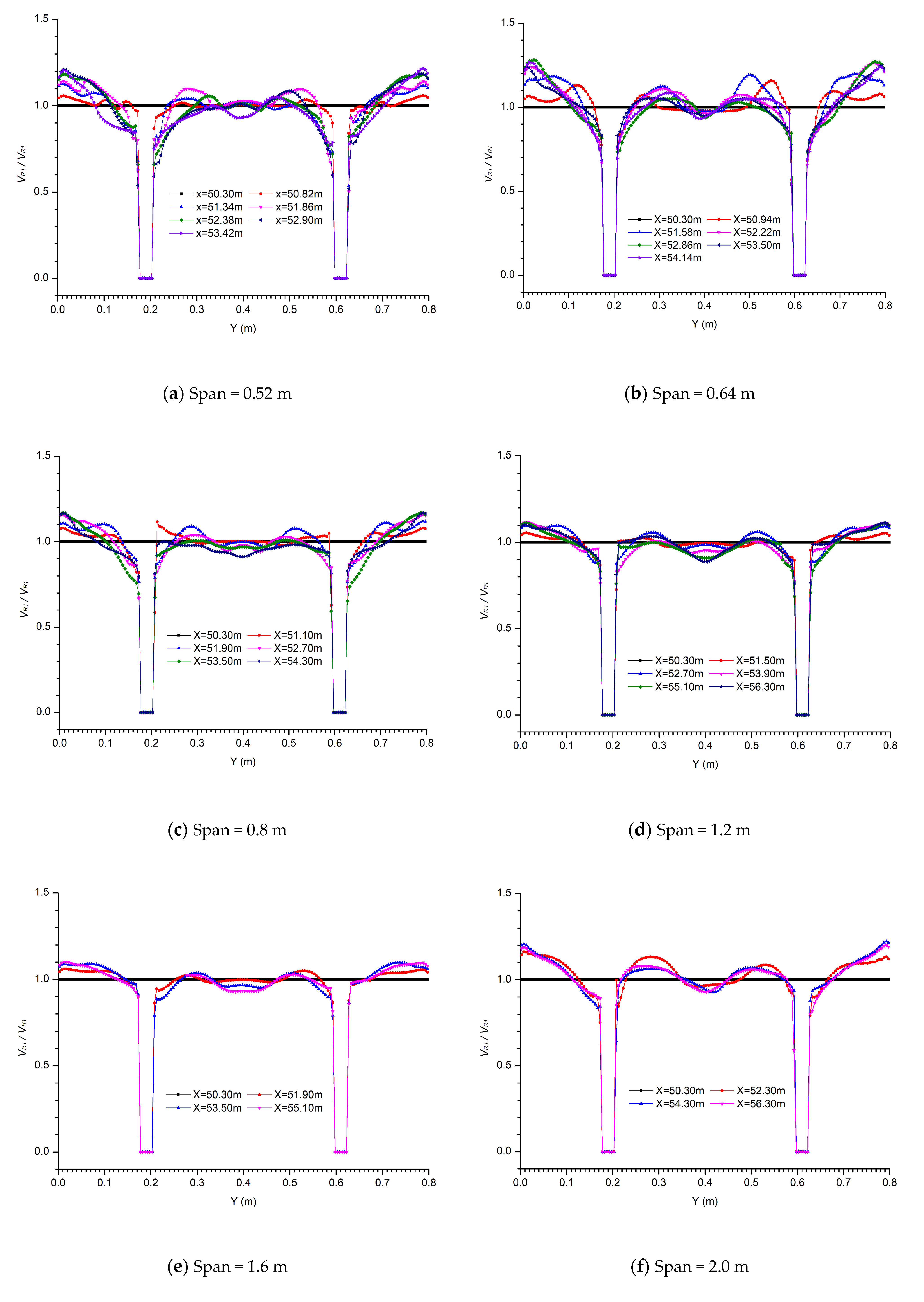
3.2. The X-Velocity of Cross-Sections in the Y-Direction

In order to obtain the characteristics of the x-velocity fields as a function of the span of piers, cross-sections at the center of each row in the x direction were selected and normalized with the velocity at the first cross-sections of each row in the different models. The normalization can show the difference of velocity affected by different spans between cross-sections. The profiles of VRi/VR1 (VRi is the x-velocity of the i-th cross-section, and VR1 is the x-velocity of the first cross-section) are plotted in Figure 11.
From the above figures, the region and the value of x-velocity in the area between the piers and the wall changed significantly compared with that of the first cross-section in each condition. The VRi/VR1 near the wall increased up to 1.26. If the span was shorter than 27.5D, the largest VRi/VR1 was around 1.17–1.26, and it was about 1.10 when the span was between 27.5D and 40D. When the span was 50D, the largest VRi/VR1 was around 1.20. In each condition, the largest VRi/VR1 at the latter piers was greater than the largest VRi/VR1 at the front piers, which reflected the accumulative influence of the superposition of Kármán Vortex Streets on the velocity. In addition, the further the location away from the first cross-section was, the more obvious the superposition of Kármán Vortex Streets on the velocity was. The increases in velocity in this area may have a negative effect on the stability of the river bank. Near each pier, the VRi/VR1 decreased. The shorter the span was, the larger the decreased region and the value of x-velocity were. For the area between the piers, the distribution shape of the VRi/VR1 changed from a “∩-shape” to an “M-shape” in each model, which indicates the value of x-velocity in the middle of each model became smaller in the x direction.

3.3. The Relationship between X-Velocity and the Span of the Pier

In order to analyze the influence of different pier spans on the x-velocity quantitatively, an average velocity change ratio (RAVC) is defined as:
RAVC = 100(V2V1)/V1
where V2 is the average x-velocity of the flow domain from x = 50 m to 27.5D downwards the last pier at z = 0.002 m and t = 50 s; V1 is the average x-velocity at x = 50 m, z = 0.002, and t = 400 s without bridge piers. RAVC of each span is shown in Table 5. RAVC values were negative, which means the x-velocities without piers were larger than these with piers. As the span increases, RAVC increased gradually and tended to be stable. The largest RAVC was about −17.66% with a span of 0.52 m, and that tended to be stable at about −11% when the span was longer than 40D. The shorter the span was, the larger the absolute value of RAVC was. With the increase of span, the RAVC of each condition became close to that of two piers gradually.
The maximum x-velocity in the longitudinal bridge section was located near the piers, and was related to the span. In order to analyze the influence of different pier spans on the maximum x-velocity at each pier quantitatively, the ratio of the maximum x-velocity among piers in each row in different models to the maximum x-velocity of two piers arranged side by side, RMV, is defined as:
R M V = M V i M V
where MVi is the maximum x-velocity among piers in each row in different models and MV is the maximum x-velocity among piers of the two piers arranged side by side, which is 0.66 m/s in this study. RMV is plotted in Figure 12.
The maximum x-velocity of the piers of the first row in each model are close to each other, which is in agreement with the results reported by Wang et al. [18]. The maximum x-velocity reduced rapidly from the 1st pier to the 2nd pier in each model, then reduced slowly from the 2nd pier to the last one, and finally became stable, especially when the span was shorter than 27.5D. If the span was longer than 27.5D, the maximum x-velocity was close to each other for the 2nd pier and the last pier. Except for the first pier in each condition, the shorter the span was, the smaller the maximum x-velocity at the same pier was.
The RMV of the piers in the first row in each model was around 0.95, which means the maximum x-velocity near the piers of the first row in each model was about 0.95 times that of the two piers arranged side by side. Then RMV reduced sharply to the second pier in each model, which was around 0.82 when the span was shorter than 27.5D, and the RMV of the second pier was up to 0.91 if the span was longer than 27.5D. If the span was longer than 27.5D, the RMV was close to each other from the 2nd pier to the last one.
Based on the discussion above, the presence of the upstream piers reduced the maximum x-velocity near the downstream piers effectively. The superposition of the vortex streets generated by tandem piers had a significant sheltering effect on the maximum x-velocity near each pier, which caused the reduction of the maximum x-velocity near each pier. With the increase of the span, the sheltering effect on the maximum x-velocity decreased gradually.

4. Conclusions

From the results presented above, the following conclusions can be drawn:
  • With a span shorter than 27.5D, the shape and the lateral range of the x-velocity increase with the increase of distance downwards the x-direction. The accumulative influence of the superposition of Kármán Vortex Streets is obvious, and the shorter the span is, the more obvious the influence of the span on the shape and width of the x-velocity is. When the span is longer than 27.5D, the accumulative effects reduce and x-velocity fields become visually almost independent of each other.
  • For the area between the piers and the wall, the VRi/VR1 near the wall increases up to 1.26. If the span is shorter than 27.5D, the largest VRi/VR1 is around 1.17–1.26, and it is about 1.10 when the span is between 27.5D and 40D. When the span is 50D, the largest VRi/VR1 is around 1.20. For the area between the two columns of tandem piers, the profile of the VRi/VR1 changes from a “∩-shape” to an “M-shape” in each model, which indicates that the value of x-velocity in the middle of each model becomes smaller in the x direction.
  • RAVC increases gradually and tends to be stable with the increases of the span. The largest RAVC is about −17.66% with a span of 0.52 m and gets close to that of two piers arranged side by side gradually with the increase of span.
  • The maximum x-velocity reduces rapidly from the 1st pier to the 3rd pier if the span is shorter than 27.5D, then slowly reduces from the 4th pier to the last one. If the span is longer than 27.5D, the maximum x-velocity is close from the 2nd pier and finally becomes stable.
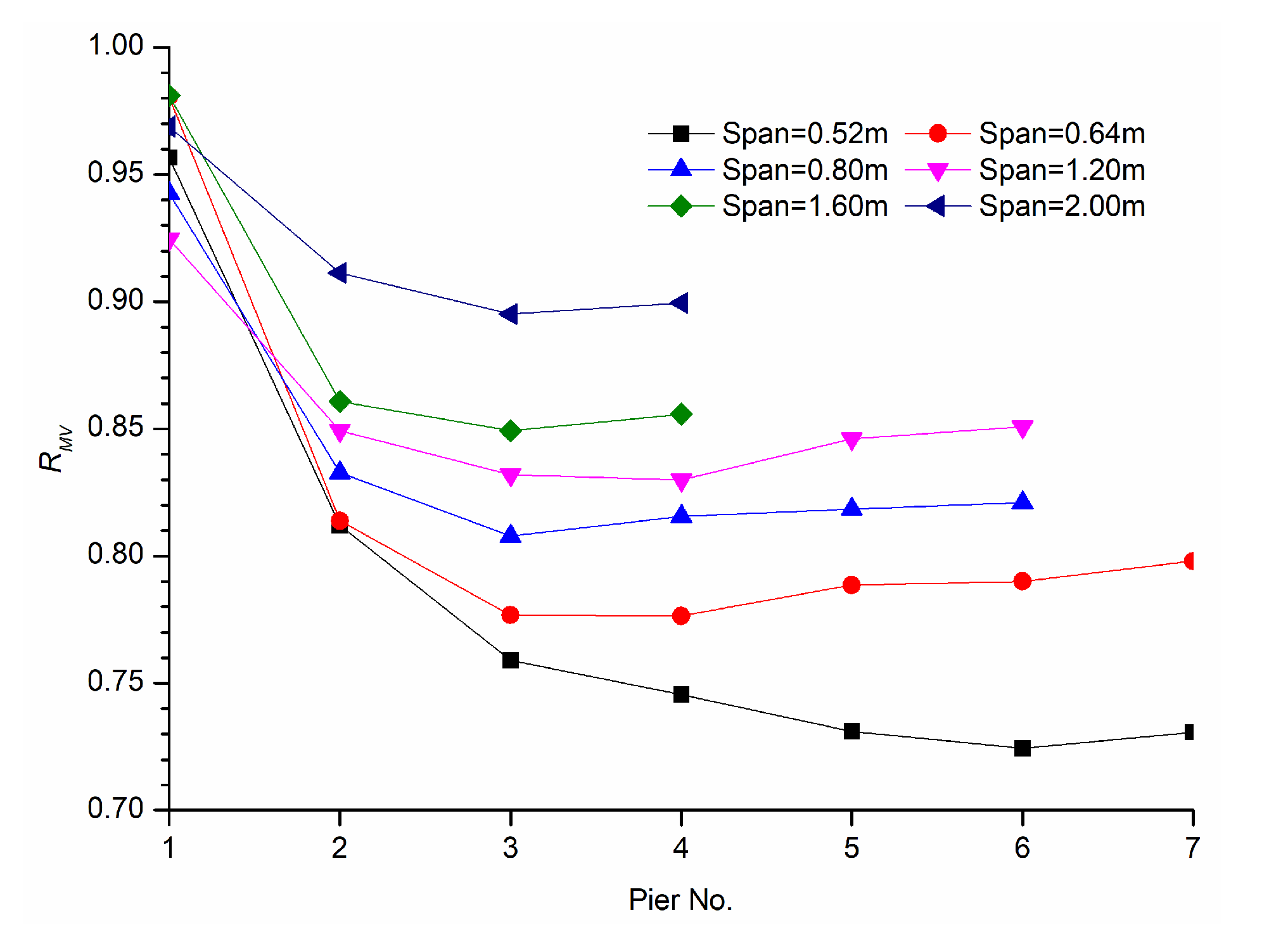
  • The RMV of the piers in the first row of different models is around 0.95, and then reduces sharply to the second pier in each model, which is around 0.82 when the span is shorter than 27.5D and up to 0.91 if the span is longer than 27.5D. If the span is longer than 27.5D, the RMV is close to each other from the 2nd pier to the last one.
This research can provide the characteristics of velocity filed near-bed region abound two columns of tandem piers of the longitudinal bridge, which could be a reference and guidance for the design of the longitudinal bridge (mainly the pier span of bridges) in mountain areas. The achievements can achieve more positive effects through wider promotions and applications.

Author Contributions

Conceptualization, H.Q.; Methodology, H.Q. and J.Z.; Software, H.Q.; Validation, H.Q., J.Z. and C.Z.; Investigation, C.Z.; Writing—original draft preparation, H.Q.; Writing—review and editing, J.Z. and C.Z.; Project administration, H.Q.; Funding acquisition, H.Q. All authors have read and agreed to the published version of the manuscript.

Funding

This research is supported by the National Natural Science Foundation for Young Scholars of China under Grant No.51708043, the Natural Science Basic Research Plan in Shaanxi Province of China under Grant No.2019JQ-680, the Special Fund for Basic Scientific Research of Central Colleges (Natural Sciences) under Grant No.300102219106, and the Program of Study Abroad for Young Scholar sponsored by the CSC (China Scholarship Council).

Acknowledgments

The authors gratefully acknowledge the support from Wen Zou and Ziheng Qi during the writing of the paper.

Conflicts of Interest

The authors declare no conflict of interest.

References

  1. Julio, S. An investigation of the wake of a circular cylinder using a video-based digital cross-correlation particle image velocimetry technique. Exp. Therm. Fluid Sci. 1996, 12, 221–233. [Google Scholar]
  2. Lin, J.C.; Rockwell, D. Horizontal oscillation of a cylinder beneath a free surface vortex formation and loading. J. Fluid Mech. 1999, 389, 1–26. [Google Scholar] [CrossRef]
  3. Breuer, M.S.; Jørgen, F. Hydrodynamics around Cylindrical Structures; World Scientific Press: Copenhagen, Denmark, 2006. [Google Scholar]
  4. Lin, J.C.; Yang, Y.; Rockwell, D. Flow past two cylinders in tandem: Instantaneous and averaged flow structure. J. Fluids Struct. 2002, 16, 1059–1071. [Google Scholar] [CrossRef]
  5. Tian, W.P.; Shen, B. Circling flow characteristics around cylinder pier. J. Xi’an Highw. Univ. 2003, 23, 54–57. [Google Scholar]
  6. He, G.J.; Fang, H.W.; Fu, R.S. Three-dimensional numerical analyses on water flow affected by piers. J. Hydrodyn. Ser. A 2007, 22, 345–351. [Google Scholar]
  7. Li, B.; Sun, D.P.; Lai, G.W. The influence of bridge pier arrangement on circling flow around bridge pier and local velocity field. China Rural Water Hydropower 2013, 129–132, 134. [Google Scholar]
  8. Kim, H.J.; Durbin, P.A. Investigation of the flow between a pair of cylinders in the flopping regime. J. Fluid Mech. 1988, 196, 431–448. [Google Scholar] [CrossRef]
  9. Gu, Z.F. On interference between two circular cylinders at supercritical Reynolds number. J. Wind Eng. Ind. Aerodyn. 1996, 62, 175–190. [Google Scholar] [CrossRef]
  10. Sumner, D.; Price, S.J.; Paidoussis, M.P. Flow-pattern identification for two staggered circular cylinders in cross-flow. J. Fluid Mech. 2000, 411, 263–303. [Google Scholar] [CrossRef] [Green Version]
  11. Meneghini, J.R.; Saltara, F.; Siqueira, C.L.R.; Ferrarijr, J.A. Numerical simulation of flow interference between two circular cylinders in tandem and side-by-side arrangements. J. Fluids Struct. 2001, 15, 327–350. [Google Scholar] [CrossRef]
  12. Li, W.W.; Huang, B.S.; Hou, J. Experimental research on hydraulic characteristics of pile wharf upon the flow of the channel. J. Xinjiang Agric. Univ. 2004, 27, 78–81. [Google Scholar]
  13. Ataie-Ashtiani, B.; Aslani-Kordkandi, A. Flow field around side-by-side piers with and without a scour hole. Eur. J. Mech. B Fluids 2012, 36, 152–166. [Google Scholar] [CrossRef]
  14. Yan, J.K.; Jiao, C.; Long, T. Bed fixed experimental study on velocity distribution of bridge piers with different intersection angles between bridge axle and flow direction. J. Xi’an Univ. Archit. Technol. 2013, 45, 822–828. [Google Scholar]
  15. Igarashi, T. Characteristics of the flow around two circular cylinders arranged in tandem. Bull. JSME 1981, 24, 323–331. [Google Scholar] [CrossRef]
  16. Mahbub, A.M.; Zhou, Y. Strouhal numbers, forces and flow structures around two tandem cylinders of different diameters. J. Fluids Struct. 2008, 24, 505–526. [Google Scholar] [CrossRef]
  17. Ataie-Ashtiani, B.; Aslani-Kordkandi, A. Flow field around single and tandem piers. Flow Turbul. Combust. 2013, 90, 471–490. [Google Scholar] [CrossRef]
  18. Wang, H.; Tang, H.W.; Xiao, J.F.; Jiang, S. Clear-water local scouring around three piers in a tandem arrangement. Sci. China Technol. Sci. 2016, 59, 888–896. [Google Scholar] [CrossRef]
  19. Chavan, R.; Kumar, B. Experimental investigation on flow and scour characteristics around tandem piers in sandy channel with downward seepage. J. Mar. Sci. Appl. 2017, 16, 313–322. [Google Scholar] [CrossRef]
  20. Beg, M.; Beg, S. Scour hole characteristics of two unequal size bridge piers in tandem arrangement. ISH J. Hydraul. Eng. 2015, 21, 85–96. [Google Scholar] [CrossRef]
  21. Schindfessel, L.; Creëlle, S.; De Mulder, T. Flow patterns in an open channel confluence with increasingly dominant tributary inflow. Water 2015, 7, 4724–4751. [Google Scholar] [CrossRef] [Green Version]
  22. Ersoy, H.; Karahan, M.; Gelişli, K.; Akgün, A.; Anılan, T.; OğuzSünnetci, M.; Yahşi, B.K. Modelling of the landslide-induced impulse waves in the Artvin Dam reservoir by empirical approach and 3D numerical simulation. Eng. Geol. 2019, 249, 112–128. [Google Scholar] [CrossRef]
  23. Oscar, H.G.; Stanisław, W.K. Numerical and physical modeling of water flow over the ogee weir of the new Niedów barrage. J. Hydrol. Hydromech. 2016, 64, 67–74. [Google Scholar]
  24. Quaresma, A.L.; Romão, F.; Branco, P.; Maria, T.F.; António, N.P. Multi slot versus single slot pool-type fishways: A modeling approach to compare hydrodynamics. Ecol. Eng. 2018, 22, 197–206. [Google Scholar] [CrossRef]
  25. Thompson, J.M.; Hathaway, J.M.; Schwartz, J.S. Three-dimensional modeling of the hydraulic function and channel stability of regenerative stormwater conveyances. J. Sustain. Water Built Environ. 2018, 4, 1–12. [Google Scholar] [CrossRef]
  26. Veksler, A.B.; Safin, S.Z. Hydraulic regimes and downstream scour at the Kama Hydropower Plant. Power Technol. Eng. 2018, 51, 491–500. [Google Scholar] [CrossRef]
  27. Morovati, K.; Eghbalzadeh, A. Study of inception point, void fraction and pressure over pooled stepped spillways using FLOW-3D. Int. J. Numer. Methods Heat Fluid Flow 2018, 28, 982–998. [Google Scholar] [CrossRef]
  28. Movahedi, A.; Kavianpour, M.R.; Aminoroayaie, Y.O. Evaluation and modeling scouring and sedimentation around downstream of large dams. Environ. Earth Sci. 2018, 77, 320–327. [Google Scholar] [CrossRef]
  29. Song, Y.; Zhang, L.L.; Li, J.; Chen, M.; Zhang, Y.W. Mechanism of the influence of hydrodynamics on Microcystis aeruginosa, a dominant bloom species in reservoirs. Sci. Total Environ. 2018, 15, 230–239. [Google Scholar] [CrossRef]
  30. Yang, S.L.; Yang, W.L.; Qin, S.Q.; Li, Q.; Yang, B. Numerical study on characteristics of a dam-break wave. Ocean. Eng. 2018, 159, 358–371. [Google Scholar] [CrossRef]
  31. Palau-Salvador, G.; Stoesser, T.; Rodi, W. LES of the flow around two cylinders in tandem. J. Fluids Struct. 2008, 24, 1304–1312. [Google Scholar] [CrossRef] [Green Version]
  32. Mohamed, H.I. Numerical simulation of flow and local scour at two submerged-emergent tandem cylindrical piers. J. Eng. Sci. 2013, 41, 1–19. [Google Scholar]
  33. Jafari, M.; Ayyoubzadeh, S.A.; Esmaeilivaraki, M.; Rostami, M. Simulation of flow pattern around inclined bridge group pier using FLOW-3D Software. J. Water Soil 2017, 30, 1860–1873. [Google Scholar]
  34. Bayon, A.; Valero, D.; García-Bartual, R.; Vallés-Morána, F.J.; López-Jiméneza, P.A. Performance assessment of Open FOAM and FLOW-3D in the numerical modeling of a low Reynolds number hydraulic jump. Environ. Model. Softw. 2016, 80, 322–335. [Google Scholar] [CrossRef]
  35. Ali, K.H.M.; Karim, O. Simulation of flow around piers. J. Hydraul. Res. 2002, 40, 161–174. [Google Scholar] [CrossRef]
  36. Calomino, F.; Tafarojnoruz, A.; De Marchis, M.; Gaudio, R. Experimental and numerical study on the flow field and friction factor in a pressurized corrugated pipe. J. Hydraul. Eng. 2015, 141, 1–23. [Google Scholar] [CrossRef]
  37. Duguay, J.M.; Lacey, R.W.J.; Gaucher, J. A case study of a pool and weir fishway modeled with open foam and FLOW-3D. Ecol. Eng. 2017, 103, 31–42. [Google Scholar] [CrossRef]
  38. Ran, D.J.; Wang, W.E.; Hu, X.T. Three-dimensional numerical simulation of flow in trapezoidal cutthroat flumes based on FLOW-3D. Front. Agric. Sci. Eng. 2018, 5, 168–176. [Google Scholar] [CrossRef] [Green Version]
  39. Nguyen, V.T. 3D numerical simulation of free surface flows over hydraulic structures in natural channels and rivers. Appl. Math. Model. 2015, 39, 6285–6306. [Google Scholar] [CrossRef]
  40. Sarker, M.A. Flow Measurement around scoured bridge piers using Acoustic-Doppler Velocimeter (ADV). Flow Meas. Instrum. 1998, 9, 217–227. [Google Scholar] [CrossRef]
  41. Breuer, M. Numerical and modeling influences on large-eddy simulations for the flow past a circular cylinder. Int. J. Heat Fluid Flow 1998, 19, 512–521. [Google Scholar] [CrossRef]
  42. Roulund, A. Three-Dimensional Numerical Modeling of Flow around a Bottom-Mounted Pile and Its Application to Scour. Ph.D. Thesis, Technical University of Denmark, Kongens Lyngby, Denmark, 2000. [Google Scholar]
  43. Roulund, A.; Sumer, B.M.; Fredsøe, J.; Michelsen, J. Numerical and experimental investigation of flow and scour around a circular pile. J. Fluid Mech. 2005, 534, 351–401. [Google Scholar] [CrossRef]
Figure 1. Longitudinal bridge piers in valleys.
Fluids 05 00032 g001
Figure 2. Local scour near longitudinal bridge piers.
Fluids 05 00032 g002
Figure 3. The profiles of x-velocity without a pier in X-Y at z = 12.75 cm and t = 400 s (unit: m/s).
Fluids 05 00032 g003
Figure 4. The profiles of x-velocity in the channel without a pier.
Fluids 05 00032 g004
Figure 5. Layout and the boundary conditions of the model with piers.
Fluids 05 00032 g005
Figure 6. The profiles of x-velocity with two piers.
Fluids 05 00032 g006
Figure 7. The velocity field around the cylinder on the bed.
Fluids 05 00032 g007
Figure 8. Of excess shear stress on the riverbed (z = 0.002 m, t = 50 s) (unit: Pa).
Fluids 05 00032 g008
Figure 9. The profiles of x-velocity in x-y at z = 0.002 m and different times with a span of 0.52 m.
Fluids 05 00032 g009aFluids 05 00032 g009b
Figure 10. The profile of x-velocity in x-y at z = 0.002 m and t = 50 s with different spans.
Fluids 05 00032 g010aFluids 05 00032 g010b
Figure 11. The profiles of VRi/VR1 at z = 0.002 m and t = 50 s with different spans.
Fluids 05 00032 g011
Figure 12. The profiles of the RMV of each pier in different models.
Fluids 05 00032 g012
Table 1. Relevant research results of the flow field characteristics around tandem piers.
SourceArrangements of PiersResults
Ataie-Ashtiani et al. [17]Two circular piers arranged in tandem
  • The presence of downstream pier changes the flow structure to a great extent, particularly in the near wake region.
  • Near the bed, the velocity of flow approaching the downstream pier decreases to 0.2–0.3 times of the approach mean velocity due to the sheltering effect of the upstream pier.
  • In the wake of the downstream pier, the flow structure is completely different from the one in the wake of a single pier.
  • In comparison with the single pier, the values of turbulence kinetic energy and turbulence intensities decrease around the tandem piers.
Wang et al. [18]Three piers arranged in tandem under steady clear-water conditions.
  • The scour-hole depth around the upstream pier was the same as that for single piers and independent of pier spacing.
  • When the spacing was larger than 11 times the diameter of a pier, the scour depths of the three-pier configuration were the same as for the single piers.
Table 2. Parameters of the model.
ItemWidth of Channel (m)Height of Channel (m)Average Velocity of Cross-Section (m/s)Initial Flow Depth (m)Pier Diameter (m)Shape of Cross-Section
Parameters 20D (0.8)6D (0.24)0.54D (0.16)0.04Rectangle
Table 3. Boundary conditions of the model.
ItemXmin (Upstream)Xmax (Downstream)YminYmaxZminZmax
Boundary conditionsvelocity (0.5 m/s)outflowwallwallwallpressure
Table 4. Parameters of the model with pier.
FactorsLevels
123456
Plane of riverstraight
Plane of bridge straight
Span of pier (m)0.520.640.801.201.602.00
Position in the river (Distance between the centerline of the model and the channel bank) (m)0.4
Table 5. RAVC of each span.
Span0.52 m0.64 m0.80 m1.20 m1.60 m2.00 m2 Piers
V2 (m/s)0.2750.2790.2800.2890.2970.2990.302
V1 (m/s)0.334
RAVC (%)−17.66−16.47−16.17−13.47−11.08−10.48−9.58

