1. Introduction
The onset of turbulence in fluids is to-date an unresolved puzzle, remaining at the focus of research in the past century partly due to its significance in engineering applications. Mathematically, a complete description of the fundamental physical problem has not yet been developed, while from a philosophical stand-point, turbulence remains a problem of determinism and chaos, a transition from laminar to turbulent flows.
The transitional two-dimensional structure that typically forms in a Blasius (laminar) boundary layer, or any other similar flow, was first observed by Ludwig Prandtl and further studied by Tollmien [
1] and Schlichting [
2] (TS). The TS instability is the initial part of the process of transition to turbulence in viscous boundary layers for which the essential mathematics was developed in the 1950 by Schlichting [
3] and inner mechanisms uncovered more recently by Baines et al. [
4]. Kachanov [
5] noted that the TS instability formation process represents the receptivity and response of a boundary layer to either external or internal perturbations. As a consequence, low-amplitude, two-dimensional and unsteady TS waves are formed that grow exponentially and, when their rotational speed reaches in magnitude about 1% or 2% of the free-stream velocity, breakdown causing the flow to become heavily three dimensional and eventually reach a fully developed turbulent state further downstream. The term fully developed turbulent regime or fully turbulent will be used here to indicate a regime when turbulence quantities no longer vary in the streamwise direction.
It is well established that the process of transition begins from very low levels of background noise. The mean flow, above a critical Reynolds number, becomes inherently unstable to small-amplitude disturbances, and the development to turbulence ensues. The transition process can be accurately described by either linear stability theory such as the Orr-Sommerfeld equation developed at the beginning of the 20th century or Floquet theory. Use of the Orr-Sommerfeld equation provides for the linear two-dimensional modes of disturbance to a viscous (NSE) parallel flow. The TS instability tends to become unstable under the conditions given by the Orr-Sommerfeld equation, initiating the transition process and eventually leading to turbulence.
It has previously been shown in various publications that temporal transition in channel flows can be simulated quite accurately by numerical means. Using direct numerical simulation (DNS), Sandham and Kleiser [
6] and Härtel and Kleiser [
7] obtained a very good prediction of the transitional flow structures present, such as the formation of
-vortices, roll-up of shear layers and appearance of hairpin vortices, while Baines et al. [
4] probed the mechanisms behind the Tollmien-Schlichting instability. Further, large eddy simulation (LES) studies conducted on grids much coarser than those required to conduct equivalent fully resolved DNS also exhibited similar transitional phenomena. See Germano et al. [
8], Schlatter et al. [
9,
10] and references therein for further details.
More recent studies by Wu and Moin [
11] and Sayadi et al. [
12], triggered transition of a weakly-compressible Blasius layer at a Mach number of 0.2, by two different instability mechanisms of TS-type transition into developed turbulence. Most importantly, it was demonstrated how boundary layers develop into a statistically self-similar and universal state independent of the transition mechanism.
More relevant to the case of bypass transition examined herein, Schlatter et al. [
13] clarified the receptivity of the boundary-layer streaks behind the turbulent breakdown of a boundary layer subject to free-stream turbulence. The rise of turbulent spots in the boundary layer were attributed to a streak secondary-instability process. Initially forming as a weak wave packet located in the low-speed streak, it begins to grow in strength while dispersing in the streamwise direction. During the breakdown to turbulence, quasi-streamwise vortex structures were identified on the flanks of the low-speed region and arranged in a staggered pattern.
A criteria for bypass transition is defined by Wu et al. [
14] as the superposition of a laminar Blasius boundary layer with a freestream of an initial turbulence intensity level,
, of approximately 1% to 4%. Their analysis elucidated how bypass transition proceeds through a sequence of characteristic structure formations: (i) formation of Lambda vortices, (ii) followed by hairpin packets, (iii) leading to infant turbulent spots, and finally (iv) hairpin forests. This sequence of events closely resembles that reported by Sayadi et al. [
15] with regards to the secondary instability and breakdown process encountered in boundary layer natural transition. Wu et al. [
14] go on to reason that
-vortices owe their formation to three-dimensional velocity perturbations interacting with the near-wall spanwise vorticity, and are thus not a result of oblique-wave excited long streaks. Though the latter can still be found, it is argued that they may not play as a dynamically important role in the bypass transition sequence as the infant turbulent spots which form earlier upstream.
Reduced basis Methods are a promising tool to analyse very complex unsteady phenomena in fluid dynamics [
16], such as transition to turbulence. They are able to extract few flow features, which might be only a mathematical abstraction that allows to express the final solution as a simple linear combination of few basis functions, but they can also have a physical meaning, as they could represent coherent structures which are responsible for fundamental behaviours [
17] (e.g., structures which cause instabilities or are associated to fundamental time frequencies present in the flow field). The present work aims at exploiting this last aspect of reduced basis methods in order to identify the most important flow features, alias modes, which are responsible for bypass type transition in a developing zero-pressure gradient boundary layer flow. In particular, Dynamic Mode Decomposition (DMD), introduced by Schmid [
18], is used as feature extraction method, since it is able to characterize the extracted flow features in terms of pure frequencies and growth/decay rates. This property makes DMD the first competitor of the Proper Orthogonal Decomposition (POD) [
19], which is able to extract a set of orthogonal basis functions that can be ordered in terms of their energetic importance, but do not carry any meaningful information about frequencies and can be misleading in identifying fundamental dynamic properties [
20].
DMD has been widely used in literature for fluid analysis [
21,
22,
23,
24]. A crucial discussion in recent literature has been how to properly select the most important dynamic modes from the entire set available, in order to have a more physical understanding of the phenomenon. The selection of DMD modes is indeed not straightforward as with other reduced basis techniques, since referring only on modes amplitudes would not take into account frequencies and growth/decay rates of the modes, which also can play an important role in the selection process. Different DMD variants have been introduced which try to overcome this limit, either trying to select the most important modes a-priori, such as optimized-DMD [
25] and sparsity promoting DMD [
26], or introducing a ranking once all the DMD modes are extracted [
27,
28].
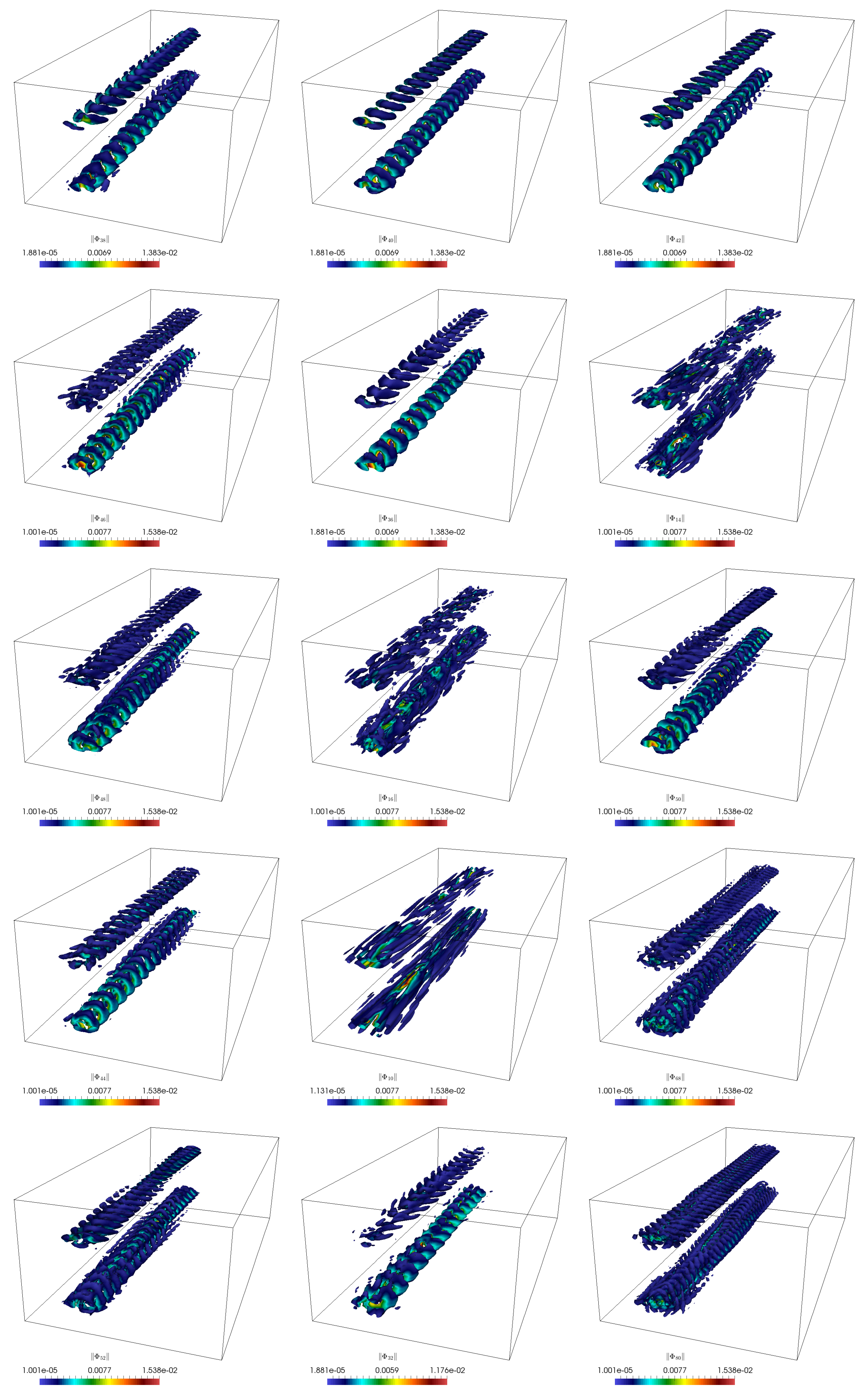
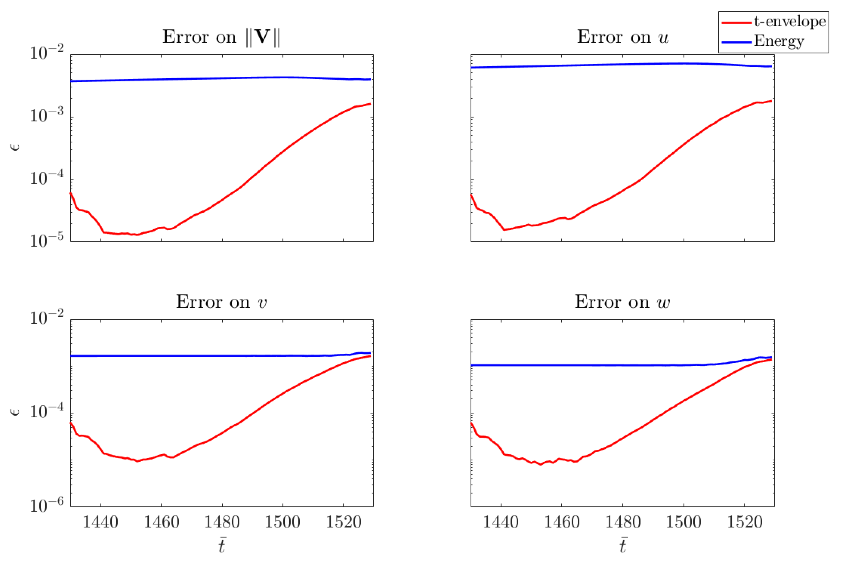
The present work aims at identifying a strategy of modes selection that will respond to two important questions: (1) can we identify DMD modes that are associated to physical flow structures that characterize the onset of transition and (2) can we identify those few DMD modes that better allow reconstructing the flow field in the region leading to the transition phase? The assessment and evaluation of DMD modes with respect to the two above criteria will be carried out by looking at the similarity between the reconstructed flow field with a few selected modes and the actual flow field in the time window preceding the actual transition zone, where turbulent structures will already show a chaotic behaviour. In this study, a first attempt is made to identify the most important modes responsible for bypass type transition in a developing zero-pressure gradient boundary layer flow using DMD equipped with a new time local selection of the most dominant modes. Since a transient phenomenon is considered, it is worth noticing here that another crucial aspect of DMD recently discussed in literature is how much it is capable to provide consistent results when transient phenomena are considered [
29]. Specifically Page and Kerswell [
30] have shown, for a simple Couette flow, how DMD can fail when trying to describe the dynamics of a fluid system moving between two equilibria along an heteroclinic orbit. Nevertheless, in the same work it was also shown how the DMD looks accurate if applied to very short time windows not containing cross-over points of the dynamical system. This is why the DMD extraction method applied in the present work is focusing on a small window at the early stage of transition. The whole transition process is indeed an heteroclinic orbit going from the unstable equilibrium of the laminar flow to the stable limit cycle of the fully-turbulent flow. Therefore, applying DMD to the entire time window is very likely to give results which are not consistent. The paper is organized as follows.
Section 2 presents the DNS-like analysis of the transition on a planar channel flow,
Section 3 reports the basics of Dynamic Mode Decomposition and its characteristics in terms of modes identification, and finally
Section 4 reports the comparative analysis and assessment of the proposed methods for modes selection in the characterization of the onset of transition.
2. Transition in a Planar Channel Flow
The numerical simulation of transition in a plane channel flow follows on from previous numerical results obtained by Kokkinakis and Drikakis [
31], where emphasis was placed solely on the final, statistically steady-state, fully turbulent regime. The purpose of this study on the contrary is to shed light into the transition process, starting from the seemingly laminar initial condition up to the fully developed turbulent state, and identify the dominant mechanisms regulating it.
The 9th-order WENO scheme and
mesh resolution are employed, for which the accuracy of the results were previously shown to be DNS–like [
31]. The Reynolds number based on the friction velocity (
) and the channel half-height (
) is equal to
, whereas that based on the bulk velocity (
) is
. The
value of the first point from the wall is equal to 0.74, resulting in a resolved mean friction Reynolds number of just over 393, within less than 0.5% of the target value. The employed grid and numerical scheme were previously shown to be capable of accurately resolving the turbulence properties of the test-case and set-up considered in this study [
31].
In order to obtain a sufficient number of flow snapshots of the bypass transition, the initial velocity field is perturbed with white noise in all directions by 5% of the local streamwise velocity (instead of the 10% used in Ref. [
31]), which in turn is obtained by a laminar Poiseuille parabolic profile. For an initial random perturbation of 1%, very weak streamwise streaks were still observed but remained inherently smooth for as long as it was computationally affordable/reasonable.
Furthermore, it was observed that a simulation’s numerical dissipation properties significantly influenced the duration of the transition process, though the underlining physical mechanism remained similar in all cases. Low-order schemes, such as the 2nd-order MC limiter, delayed the formation and appearance of the streamwise streaks while substantially decreasing their growth rate. The increased numerical dissipation of lower-order schemes severely dampens the initial perturbations, thus delaying the onset of the streamwise streaks. On the contrary, the higher-order schemes better resolve the initial random velocity perturbations and retain a much higher turbulent intensity. In either case, the disturbances resolved near the midstream are carried towards the near-wall region as momentum is transferred between the two regions during the evolution of the laminar boundary layer (BL), leading eventually to the formation of the streamwise streaks.
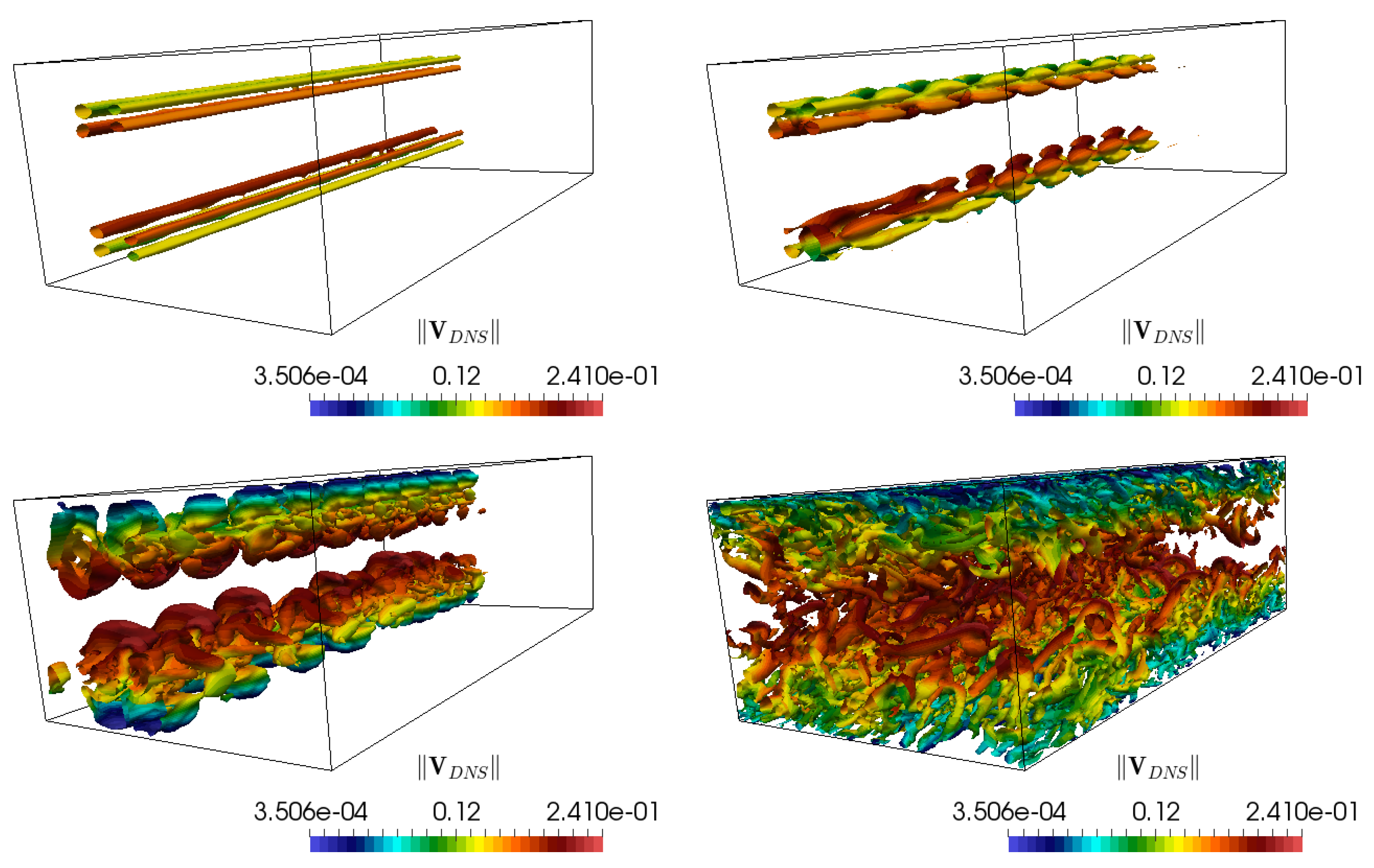
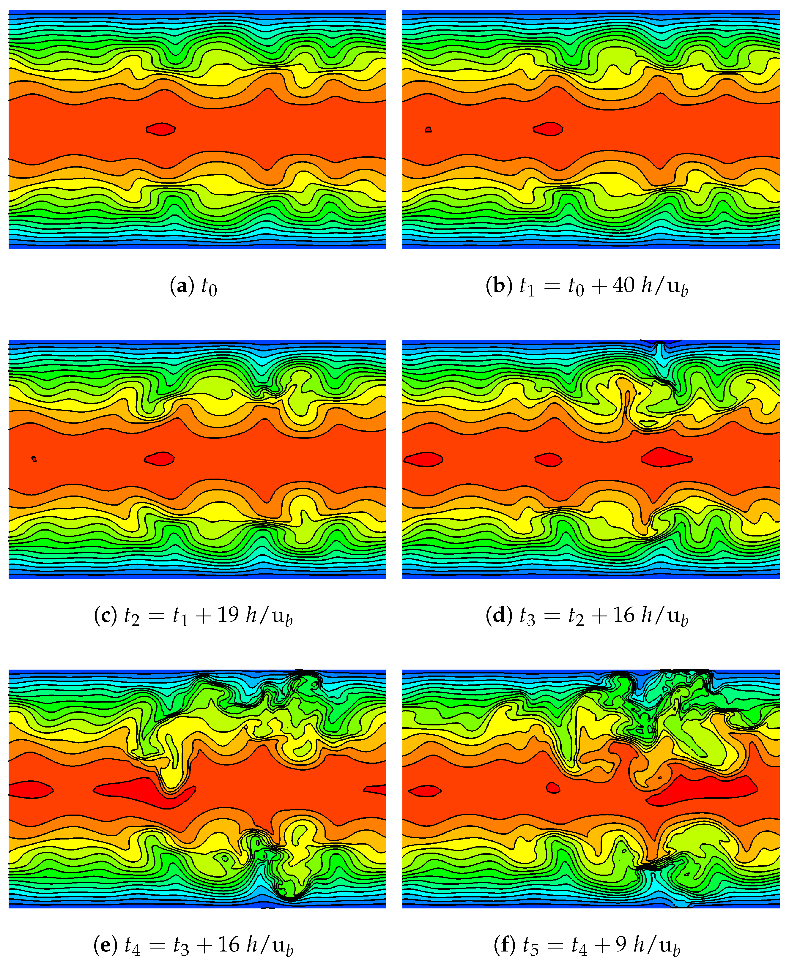
Figure 1 reports snapshots of the DNS-like solution.
2.1. Streamwise Streaks
Helicity is a scalar quantity defined as the inner product between the velocity and vorticity vectors. By definition, helicity vanishes in two-dimension. The physical meaning of helicity becomes a bit more clearer when it is normalized, defined as:
where
is the velocity vector,
is the vorticity vector and
represents their magnitude. The value of normalized helicity ranges from –1 to 1. As normalized helicity physically represents the value of the cosine angle between the velocity vector and vorticity vector, the extreme values of −1 and 1 represent regions of a flow that is highly three-dimensional, whereas the centre value of zero corresponds to a two-dimensional flowfield where the vorticity is normal to velocity, as shown in
Figure 2 where vorticity is streamwise.
Normalized helicity (Degani et al. [
32]) is a useful indicator of how the velocity vector field is oriented with respect to the vorticity vector-field for a given flowfield. For instance, at the centre of streamwise vortices and streaks, such as TS waves or streamwise streaks, the velocity and vorticity vector tend to align themselves parallel to each other and as a result the normalized helicity will attain it’s maximum absolute value of one. This fact is utilized to locate the core of unidirectional vortices such as Görtler or TS waves, as well as streamwise streaks.
Figure 2 depicts the normalized helicity prior to transition of the flowfield resolved in the Implicit Large Eddy Simulation (ILES) results.
One possible transition process is widely known as bypass transition. Under a sufficiently high level of free-stream turbulence intensity, generally >1%, streamwise elongated disturbances are induced in the near-wall zone of an attached laminar BL, termed streamwise streaks or Klebanoff distortions, such as those visualized in the top-left image of
Figure 1. Under sufficient background noise, the streaks can form in a laminar BL, and are characterized by high and low velocity that alternate in the spanwise direction (wobble) at some distinguished periodicity and with a wavelength in the order of the BL thickness
. For the channel flow at a
considered here, the streaks are positioned at
.
Landahl [
33] presumed the presence of a lift-up effect to explain the presence of streaks in transitional flows. It is argued that coherent streamwise streaks can efficiently extract energy from the mean flow via the lift-up effect, gradually strengthening and growing. This mechanism is reported to occur for spanwise scales ranging from those of the near-wall streaks (∼
) to those of the large-scale motions. The lift-up effect alone however does not determine the streak patters that emerge during transition. Using numerical results, Chernyshenko and Baig [
34] showed that the combine action of the lift-up of the mean profile, mean shear, and viscous diffusion own different streak pattern-forming properties and bear much greater influence than the pattern of the wall-normal motions. For further details concerning the lift-up effect, a recent and thorough review is given by Brandt [
35].
Typically, in a nominally zero-pressure gradient boundary layer subject to high levels of free stream turbulence, the mechanism of Tollmien–Schlichting waves transition is bypassed. Nonetheless, during the transition window, it is evident that a mean streamwise momentum transfer from the outer- towards the inner-boundary layer region still occurs. This is attributed to the streamwise streaks contained within of the boundary layer.
The wavelength of the initial streak disturbance is largely determined by low-frequency disturbances; high-frequency disturbances are mostly damped by the laminar shear layer. Once the laminar BL is distorted by the streaks, it becomes susceptible to instabilities. Although the streaks are of a large wavelength, the instabilities that form are of a short wavelength (top-right image in
Figure 1), and suggests that they are excited/triggered by high-frequency perturbations. Two of the most noteworthy instability modes are the (i) sinuous mode, and (ii) varicose mode.
The Klebanoff distortions grow downstream both in length and amplitude and finally cause breakdown–of the seemingly laminar BL to this point–with the formation of turbulent spots. These turbulent spots coalesce farther downstream, finally leading to the onset of turbulence, as indicated by the left and right bottom images in
Figure 1.
Note that besides the magnitude of the initial condition velocity perturbation, the streamwise streaks peaks and growth-rate are also sensitive to the shape of the imposed energy spectrum and its integral length scale; for the same initial velocity perturbation, or turbulence intensity , but different different , a different transition process may be obtained.
2.2. Flowfield Structure
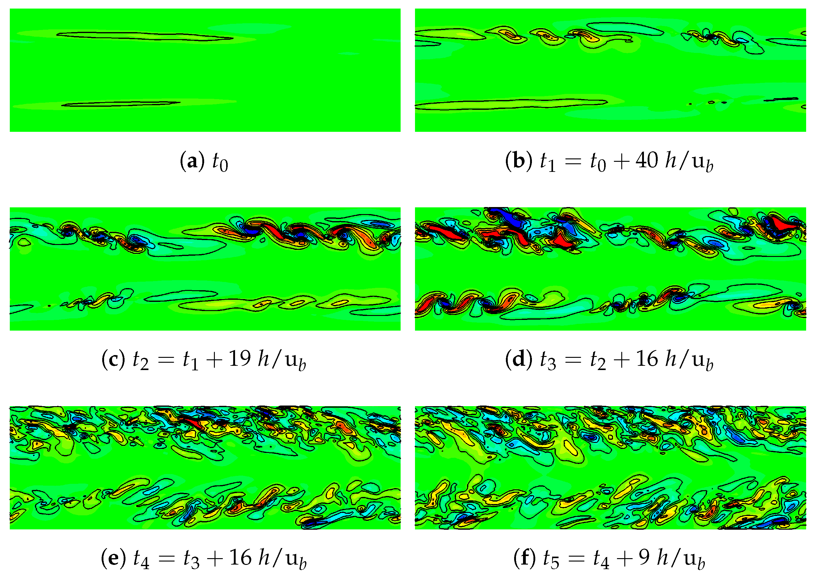
Figure 3d reports the streamwise velocity in the y-z plan at different instants of time:
,
,
,
and
, while wall-normal velocity is presented in
Figure 4. Two different 2-dimensional phenomena can be observed to have formed at the exact time the streamwise streaks begin to breakdown. One is a Rayleigh–Taylor instability (RTI) visible near the upper wall, whereas a Kelvin–Helmholtz instability (KHI) like vortex can be observed at the lower half of the channel. These typically form between two streamwise streaks that have become sufficiently strong to interact and alter one another. Asymmetries in the structure between the two streamwise streaks begin to amplify any velocity perturbations, and breakdown of the structures becomes iwhichmminent. This is also indicated by the bottom-left image in
Figure 1, along the streamwise direction.
Since the streamwise streaks are located close to each other and are located at a similar distance from the wall, the spanwise velocity perturbations are the first to be amplified—not being restricted by the presence of the wall or the proximity of the viscous sublayer. Simultaneously, the helicity structures appear to move in a side-to-side snake-like fashion in the spanwise direction, which is unrestricted in comparison to the wall-normal direction. Eventually, once the viscous shear stresses are overcome, the spanwise collision between two streaks causes momentum to be ejected in a manner resembling that of the mushroom shape typically encountered in RMI. It can therefore be deduced that prior to the RT-instability formation, streamwise streaks breakdown due to asymmetries in their structure arising from the superimposed random perturbations in the initial condition.
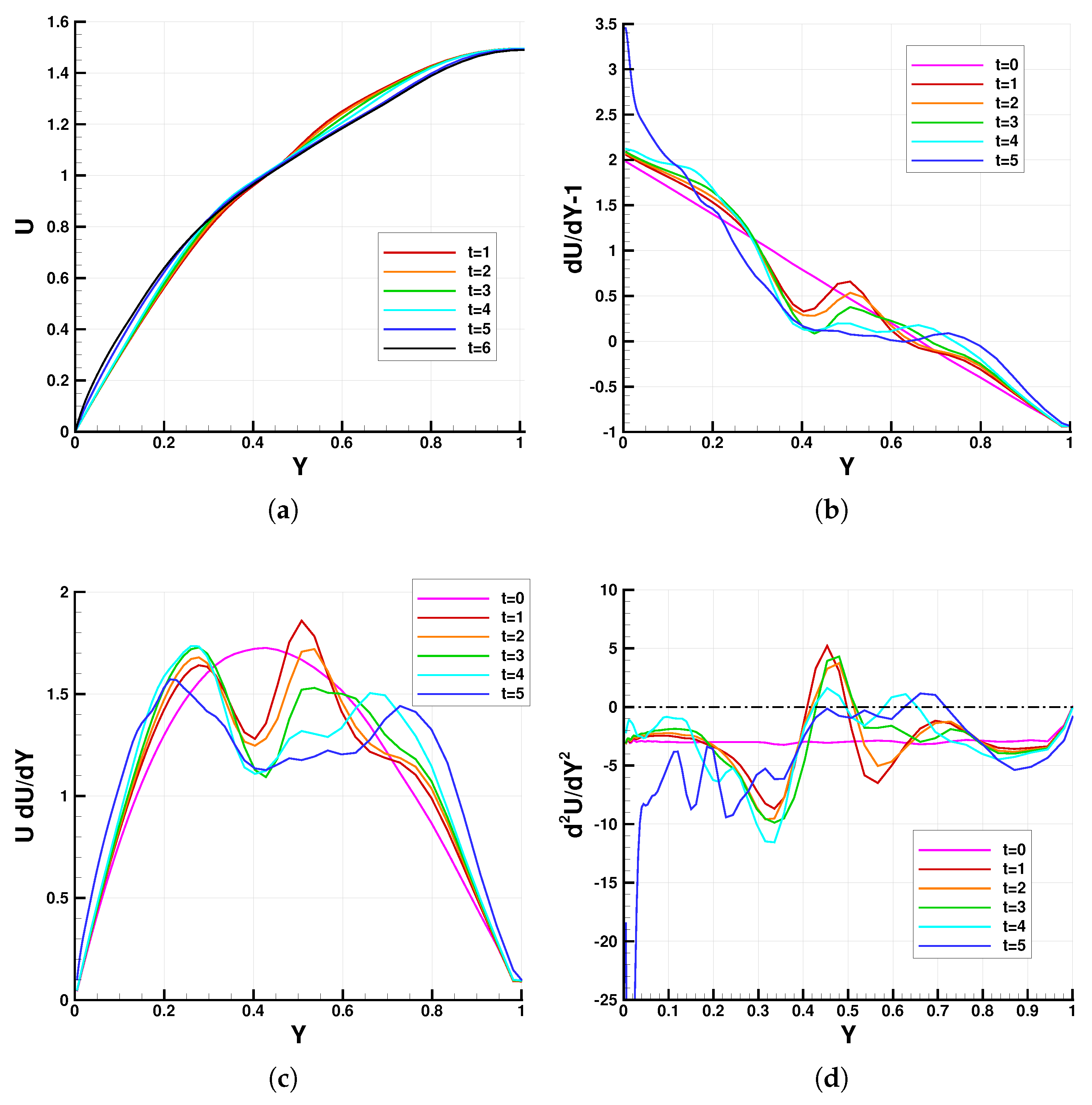
Once a streamwise streak disperses, the rest of the domain undergoes bypass transition to turbulence. It should be noted that the process of the formation of the streamwise streaks occurs while there is a gradual transfer of momentum from the upper midstream region of the boundary layer, towards the lower near wall region as can be seen in
Figure 5a, which has also been reported in the DNS of Sandham and Kleiser [
6], Härtel and Kleiser [
7]. The streamwise streaks form while the laminar boundary layer is developing; the viscous laminar boundary layer in conjunction with perturbations are responsible for a momentum exchange between the midstream and near wall region of the boundary layer.
Interest to develop methods capable of suppressing near-wall turbulence in boundary layers in order to reduce friction drag has recently highlighted the importance of the lateral oscillations exhibited by streamwise streaks prior to breakdown. In recent DNS studies conducted to develop and examine such methods, spanwise oscillatory wall motion was introduced in a fully developed turbulent channel flow (see Touber and Leschziner [
36], Lardeau and Leschziner [
37] and references therein). It was found that the unsteady cross-flow straining causes major spanwise distortions to near wall streak structures, leading to a pronounced reduction in wall-normal momentum exchange in the viscous sublayer, successfully disrupting the turbulence contribution to the wall shear stress.
Closer examination of the data reveals that the point at which the RT-instability forms is an inflection point in the streamwise velocity profile (see
Figure 5d), which is verified by transition theory. This creates two distinct regions in the laminar boundary layer that resemble a shear layer. Hence, the turbulent spots that appear in the wall-normal velocity in
Figure 4c,e are reminiscent of transition vortex spots in a turbulent free shear layer. It can therefore be concluded: (i) viscosity causes the formation of the laminar BL, (ii) within which the streamline streaks form given sufficient external perturbation, leading to a gradual momentum transfer within the laminar BL, (iii) until the Euler, or inviscid non-linear advective part of the full NSE, induces the instability breakdown mechanisms once sufficient momentum is transferred to overcome the viscous shear stresses.
3. Feature Extraction and Dynamic Mode Decomposition
Given the set of snapshots
computed through the numerical simulation and
, the variable to be processed at time
(snapshot
i), the DMD extraction technique is based on the following assumption:
which defines the linear dynamics that best fits the initial set of snapshots. This assumption allows to express the initial set of collected snapshots according to the linear dynamic theory:
where
are the vectors of DMD modes,
are the DMD eigenvalues,
are the modes amplitudes, constant in time. For an in-depth description of the DMD algorithm used in the present work to extract DMD modes the reader can refer to [
38]. The main steps are briefly presented below. An eigenvalue decomposition of the matrix
needs to be performed in order to extract DMD modes. Since for fluid dynamics problems this matrix might be huge, its dimension needs to be reduced before performing such a step. Therefore the following similarity transformation is applied to the matrix
:
where
represents the matrix of spatial functions needed to project the low-rank dynamics back to the high-dimensional space and is computed from the singular value decomposition of the matrix of snapshots
:
The last snapshot is not included in the matrix
in order to build the time shifted matrix
which allows to express Equation (
2) in matrix form:
The combination of Equations (
4)-(
6) provides an expression for the reduced matrix
:
which is usually many order of magnitude smaller than the matrix
. The singular value decomposition of matrix
might allow to perform a further reduction considering only the first
r columns of
, if a singular value threshold can be computed and all the singular values below this threshold are discarded [
39]. Nevertheless, in the present work, no reduction is introduced at this stage and all the singular vectors are considered, in order to prevent any possibility of excluding spatial functions which have very low energetic content but still have an important contribution for the dynamic. The reduced matrix
is then used to compute the eigenvalue decomposition and the spatial DMD modes can be recovered projecting back to the high-dimensional space the
eigenvectors, using the following transformation:
where
are the eigenvectors of the matrix
, also called DMD eigenvectors. The modes computed with this relation are also known as exact DMD modes [
38].
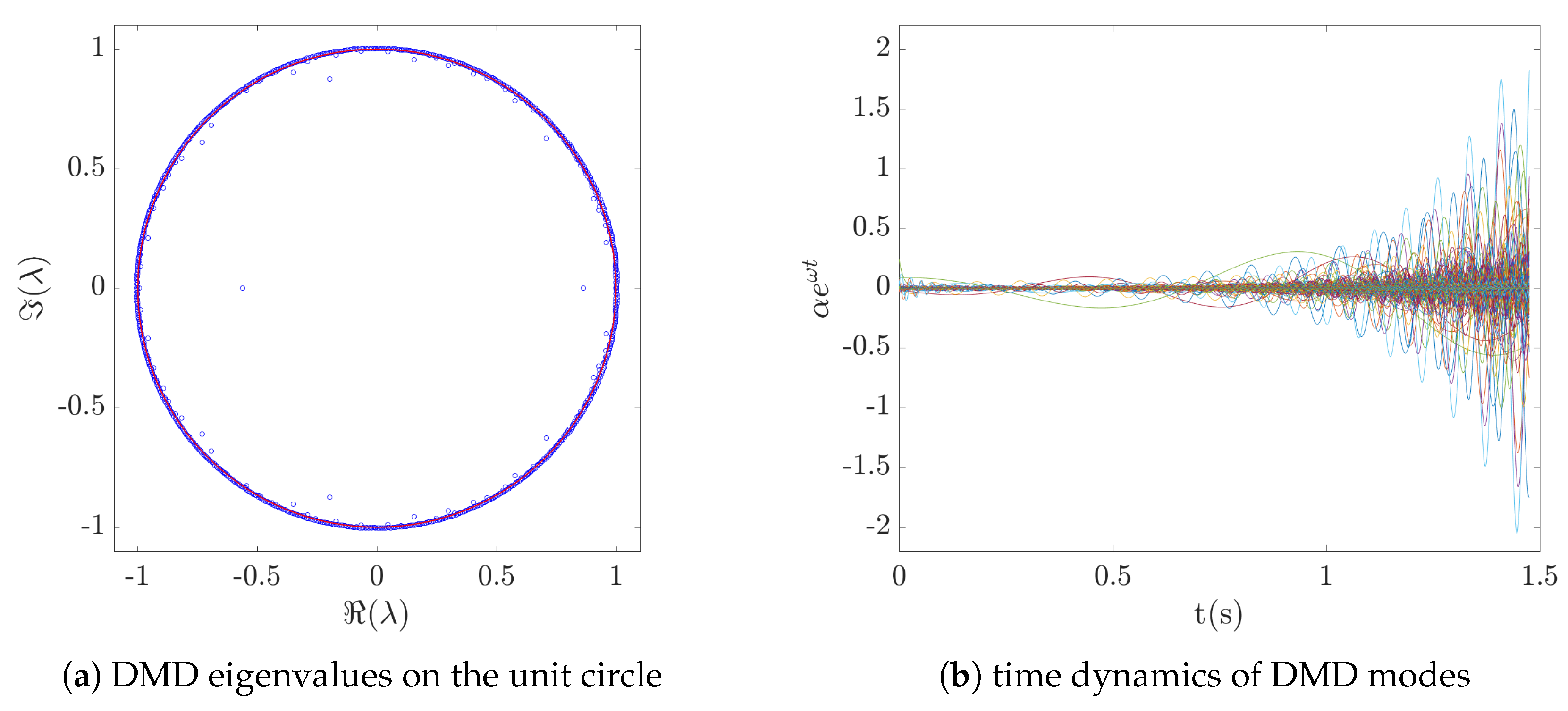
The eigenvalues of the matrix provide the growth/decay rate (real part) and the frequency (imaginary part) of each dynamic mode, and therefore define the time dynamics.
They are related to the eigenvalues
in the Equation (
3) as follows:
where
represents the physical time interval used to sample the snapshots collected in the matrix
.
The coefficients
in the Equation (
3) are computed solving the following optimization problem [
26]:
where
is the diagonal matrix of DMD coefficients
,
r is the number of DMD modes extracted, and
is the Vandermonde matrix which contains the DMD eigenvalues and is defined as follows:


